Efficient Stochastic Simulations of Complex Reaction Networks on Surfaces
Abstract
Surfaces serve as highly efficient catalysts for a vast variety of chemical reactions. Typically, such surface reactions involve billions of molecules which diffuse and react over macroscopic areas. Therefore, stochastic fluctuations are negligible and the reaction rates can be evaluated using rate equations, which are based on the mean-field approximation. However, in case that the surface is partitioned into a large number of disconnected microscopic domains, the number of reactants in each domain becomes small and it strongly fluctuates. This is, in fact, the situation in the interstellar medium, where some crucial reactions take place on the surfaces of microscopic dust grains. In this case rate equations fail and the simulation of surface reactions requires stochastic methods such as the master equation. However, in the case of complex reaction networks, the master equation becomes infeasible because the number of equations proliferates exponentially. To solve this problem, we introduce a stochastic method based on moment equations. In this method the number of equations is dramatically reduced to just one equation for each reactive species and one equation for each reaction. Moreover, the equations can be easily constructed using a diagrammatic approach. We demonstrate the method for a set of astrophysically relevant networks of increasing complexity. It is expected to be applicable in many other contexts in which problems that exhibit analogous structure appear, such as surface catalysis in nanoscale systems, aerosol chemistry in stratospheric clouds and genetic networks in cells.
pacs:
05.10.-a,82.65.+r,98.58.-wI Introduction
The catalysis of chemical reactions by surfaces plays a crucial role in a vast range of physical, chemical and biological systems. In many cases, the surfaces are of macroscopic dimensions and the reactants appear in large quantities. Under these conditions, the law of large numbers applies and fluctuations in the surface concentrations of reactants and their reaction rates become negligible. As a result, these reactions can be analyzed using rate equation models that incorporate the mean-field approximation and ignore fluctuations.
Consider the case of a surface, which is partitioned into microscopic domains, that are disconnected, namely reactants cannot diffuse between them. The population of reactive atoms and molecules in each domain becomes small and fluctuations become important. As a result, rate equations fail and the simulation of these reactions requires stochastic methods such as direct integration of the master equation vanKampen1981 ; Oppenheim1977 ; Karlin1998 ; Nasell2001 or Monte Carlo (MC) simulations Gillespie1977 ; Newman1999 . While MC simulations require the accumulation of statistical data over long times, the master equation provides the probability distribution from which the reaction rates can be obtained directly. In certain cases, the master equation can be solved using a generating function McQuarrie1963 ; McQuarrie1964 ; Gardiner1985 ; Assaf2006 ; Assaf2007 . The set of coupled ordinary differential equations is then transformed into a single partial differential equation for the generating function. This equation can solved numerically and in a few cases can also be solved analytically Green2001 ; Biham2002 . The master equation can also be approximated using the Fokker-Planck equation Montroll1946 . This is a partial differential equation in which the population sizes of the reactive species are represented by continuous variables Kolmogorov1931 . The master equation and related methods described above are useful for simple reaction networks, which involve few reactive species. However, as the number of reactive species increases, the number of equations in the master equation quickly proliferates. This makes the master equation infeasible for complex networks including a large number of reactive species.
The recently introduced multiplane method provides a dramatic reduction in the number of equations Lipshtat2004 . In this method, the reaction networks are described by graphs, where each node represents a species and each edge represents a reaction. Typically, these networks are sparse, namely most species react only with few other species. In the multiplane method one breaks the network into a set of fully connected subnetworks (cliques). Lower-dimensional master equations are constructed for the marginal probability distributions associated with the cliques, with suitable couplings between them. This enables the simulation of large networks much beyond the feasibility limit of the master equation. However, it turns out that the construction of the multiplane equations for complex networks is difficult.
In this paper we present a method for stochastic simulations of surface reaction networks, which is based on moment equations. This method exhibits crucial advantages over the multiplane method Barzel2006 . The number of equations is further reduced to one equation for each reactive species (node) and one equation for each reaction (edge). Thus, for typical sparse networks the complexity of the stochastic simulation becomes comparable to that of the rate equations. Unlike the master equation (and the multiplane method) there is no need to adjust the cutoffs, namely the same set of equations is used under all physical conditions. Moreover, for any given network the moment equations can be easily constructed using a diagrammatic approach. This enables to automate the construction of the set of equations - a feature which is essential in the case of complex networks. Furthermore, the moment equations are linear in terms of the moments. Thus, the stability and convergence properties can be easily controlled and the steady state solution can be obtained by standard algebraic methods.
Below we consider some examples of surface reaction systems in which fluctuations play an important role. In surface catalysis systems, the surface is often partitioned into facets on nanometric dimensions, with little diffusion between the facets. Under these conditions the number of reactive atoms and molecules residing on a facet is small and fluctuations are strong. Suchorski1998 ; Suchorski1999 ; Suchorski2001 ; Johanek2004 ; Pineda2006 ; Liu2002 . Another important example of chemical reaction networks that require stochastic analysis appears in the field of interstellar chemistry. Some chemical reactions in interstellar clouds take place on the surfaces of dust grains Spitzer1978 ; Hartquist1995 ; Hasegawa1992 ; Herbst1995 . These include molecular hydrogen formation Gould1963 ; Hollenbach1970 ; Hollenbach1971a ; Hollenbach1971b as well as reaction networks that form ice mantles and certain organic molecules. Unlike gas phase reactions in cold clouds that mainly produce unsaturated molecules Herbst2005 , surface processes are dominated by hydrogen-addition reactions that result in saturated, hydrogen-rich molecules, such as water (H2O), ammonia (NH3), methane (CH4), formaldehyde (H2CO) and methanol (CH3OH) Hiraoka1998 ; Hidaka2004 . In particular, recent experiments have shown that methanol cannot be efficiently produced by gas phase reactions Geppert2006 . On the other hand, there are indications that it can be efficiently produced on ice-coated grains Watanabe2005 . Therefore, the ability to perform efficient simulations of chemical reactions on interstellar grains is of great importance.
Due to the submicron size of the grains and the low gas density, the populations of reactive species per grain are small and strongly fluctuate. Therefore, rate equations are not suitable Tielens1982 ; Charnley1997 ; Caselli1998 ; Shalabiea1998 and stochastic methods such as the direct integration of the master equation Biham2001 ; Green2001 or MC simulations Charnley2001 are required. As discussed above, these methods apply in the case of small networks but become infeasible for large networks Stantcheva2002 ; Stantcheva2003 .
Here we demonstrate the moment-equation method for a set of astrophysically relevant networks of increasing complexity, culminating in the network that describes the production of methanol. It is shown that in spite of the small number of equations and the ease of their construction, the accuracy of the results is not compromised. The results of the moment equations are in excellent agreement with the master equation and coincide with the rate equations in the limit of large grains.
The paper is organized as follows. In Sec. II we consider the production rate of molecular hydrogen using the rate equation, master equation and moment equation methods. In Sec. III we consider the simulation of complex reaction networks using the moment equations. The construction of the set of moment equations using diagrammatic methods is presented in Sec. IV, followed by a summary in Sec. V.
II Molecular Hydrogen Formation
II.1 Rate Equations
Consider the reaction HHH2 that takes place on the surfaces of interstellar dust grains. Hydrogen atoms from the gas phase collide and stick to the surface of a dust grain. They diffuse between adsorption sites on the surface and when two of them encounter each other they recombine and form an H2 molecule, which desorbs into the gas phase.
For simplicity, we assume that the grains are spherical and denote their diameter by . The cross-section of a grain is and its surface area is . The density of adsorption sites on the surface of a grain is denoted by (sites cm-2). Thus, the number of adsorption sites on the grain is . Each grain is exposed to a flux (s-1) of H atoms, where (cm-3) is the density of H atoms in the gas phase and (cm s-1) is their average velocity, which is determined by the gas temperature. It is also useful to define the flux in units of monolayers (ML) per second, namely (ML s-1). Clearly, this flux is independent of the grain size.
The desorption rate of H atoms from the grain is given by , where is the attempt rate (standardly taken to be s-1), is the activation energy barrier for desorption of an H atom, and (K) is the surface temperature. The hopping rate of adsorbed atoms between adjacent sites on the surface is , where is the activation energy barrier for hopping of the atoms.
Molecular hydrogen formation on astrophysically relevant surfaces of silicates, carbon and ice has been studied by laboratory experiments during the past decade Pirronello1997a ; Pirronello1997b ; Roser2002 ; Hornekaer2003 ; Hornekaer2005 ; Vidali2005 ; Amiaud2006 . From the results of these experiments one can extract, for each surface, the energy barriers defined above and the density of adsorption sites. In the simulations presented below, the density of adsorption sites was (sites cm-2), the activation energies were meV for diffusion and meV for desorption. These parameters are rounded values of the experimental results for hydrogen recombination on silicates Katz1999 . The grain temperature was taken as K. Here we assume that diffusion occurs only by thermal hopping, in agreement with the experimental results Katz1999 ; Perets2005 . For small grains, it is convenient to replace the hopping rate (hops s-1) by the sweeping rate , which is approximately the inverse of the time it takes for an H atom to visit nearly all the adsorption sites on the grain surface (for a more precise evaluation of the sweeping rate see Refs. Krug2003 ; Lohmar2006 ). The rate equation for this reaction takes the form
| (1) |
where is the average population size of H atoms residing on the grain. The first term on the right hand side of Eq. (1) describes the incoming flux of H atoms. The second term accounts for the desorption of H atoms from the surface, which is proportional to the number of adsorbed atoms. The third term accounts for the depletion in the population of adsorbed H atoms due to the recombination process.
The production rate of H2 molecules on a single grain, is given by
| (2) |
For simplicity we assume that these molecules desorb from the surface upon formation.
The rate equation (1) can be solved either analytically or by numerical integration. The steady state solution can be obtained by setting the left hand side of Eq. (1) to zero. Under steady state conditions, the average population size of H atoms on a grain is
| (3) |
and the formation rate of molecules per grain is
| (4) |
where . Note that is independent of the grain size. Under these conditions, one can define the recombination efficiency
| (5) |
which is the fraction of adsorbed atoms that come out in molecular form. Note that .
One can identify two limits. In the limit where the desorption process is dominant and the recombination efficiency is low. In this case, the recombination rate per grain is and the recombination efficiency is . Since depends quadratically on the flux, this regime is referred to as second order kinetics. In the opposite limit, where , the recombination process is dominant and the efficiency is . This is the regime of first order kinetics, in which depends linearly on Biham1998 ; Biham2002 .
Under given flux and surface temperature, for grains that are large enough to hold many H atoms, Eq. (1) provides a good description of the recombination process. However, in the limit of small grains and low flux, may be reduced to order unity or less. Under these conditions, Eq. (1) becomes unsuitable, because it ignores the discrete nature of the population of adsorbed atoms and its fluctuations.
II.2 The Master Equation
To account correctly for the recombination rate on small grains, simulations using the master equation are required. The dynamical variables of the master equation are the probabilities of having a population of hydrogen atoms on the grain. In the case of hydrogen recombination, the master equation takes the form
| (6) | |||||
where . The first term on the right hand side of Eq. (6) describes the effect of the incoming flux. The probability increases when an H atom is adsorbed by a grain that already has adsorbed H atoms, and decreases when it is adsorbed on a grain with atoms. The second term accounts for the desorption process. The third term describes the recombination process. The recombination rate is proportional to the number of pairs of H atoms on the grain, namely . Therefore, the H2 production rate can be expressed in terms of the moments of as
| (7) |
In numerical simulations the master equation must be truncated in order to keep the number of equations finite. A convenient way to achieve this is to assign an upper cutoff on the population size. The number of equations is thus . The truncated master equation is valid if the probability to have a larger population than the assigned cutoff is vanishingly small. Therefore, the upper cutoff should be chosen according to the parameters of the simulation.
II.3 The Moment Equations
As noted above, the population size of the adsorbed H atoms is given by the first moment of , while the reaction rate can be expressed in terms of the difference between the second moment and the first moment. Therefore, a closed set of equations for the time derivatives of these first and second moments could directly provide all the information that we need about the population size and reaction rates Lipshtat2003 . Such equations can be obtained from the master equation using the identity
| (8) |
where is an integer. Inserting according to Eq. (6), one obtains the moment equations
| (9) |
This is a set of coupled differential equations, which are linear in the moments . Although we have written the equations only for the first two moments, the right hand side includes the third moment for which we have no equation. In order to close the set of equations one must express the third moment in terms of the first two moments. Different such expressions have been proposed. For example, in the context of birth-death processes the relation was used McQuarrie1967 . This choice makes the moment equations nonlinear, with possible effects on their stability. Another common choice is to assume that the third central moment is zero (which is exact for symmetric distributions) and use this relation in order to express the third moment in terms of the first and second moments Gomez-Uribe2007 .
Here we set up the closure condition by imposing a highly restrictive cutoff on the master equation. The cutoff is set at . This is the minimal cutoff that still enables the recombination process to take place. Under this cutoff, one obtains the following relation between the first three moments Lipshtat2003
| (10) |
Using this result, one can bring the moment equations [Eq. (9)] into a closed form:
| (11) |
Numerical integration of these equations provides the first two moments, from which the population size and reaction rate are obtained. The steady state solution of the moment equations can be obtained by setting the derivatives on the left hand side of Eq. (11) to zero. One obtains
| (12) |
Using Eq. (7) we find that the recombination rate is
| (13) |
In this system one can identify two characteristic spatial scales, namely and Lipshtat2003 . The limit of small grains is obtained when is smaller than both and . In this limit the populations size of atoms on the grain is small, the rate equation fails while the moment equations are accurate. The limit of large grains is obtained when is larger than both and . In this limit the population size of atoms on the grain is large, the rate equation applies and the reaction rate satisfies . Since and , the limit of large grains can be expressed by
| (14) |
We recall that the moment equations were derived by imposing a strict cutoff on the master equation. One may thus expect that the equations will apply only in the case of small grains, where this cutoff is suitable. However, it turns out that the moment equations are valid much beyond this limit. Below we show that the reaction rate obtained from the moment equations is accurate for both small and large grains.
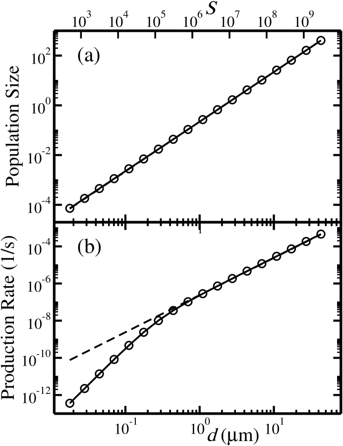
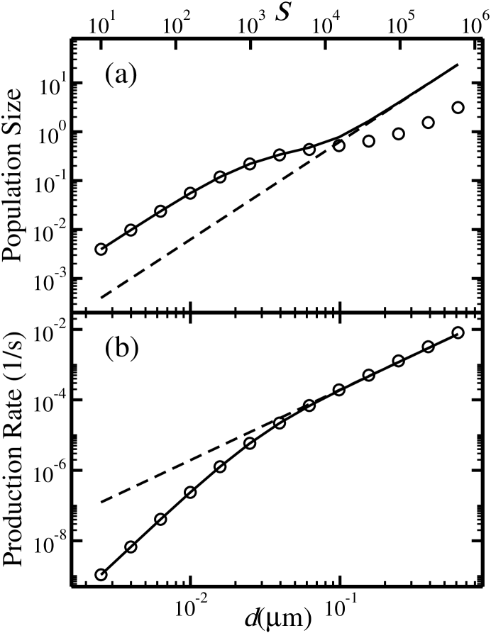
In Fig. 1 we present the population size of H atoms and the reaction rate, vs. grain diameter, obtained by the moment equations (circles). The flux of H atoms was (atoms s-1). The parameters used in Fig. 1 satisfy the conditions for second-order kinetics, namely . The results are in perfect agreement with the master equation (solid lines) for the entire range of grain sizes. For small grains, the rate equation (dashed lines) over-estimates the recombination rate, but coincides with the master equation and the moment equations for large grains. In Fig. 2 we present the population size of H atoms and the reaction rate, vs. grain diameter, under the conditions of first-order kinetics, where . These conditions were obtained by increasing the flux to (atoms s-1). The moment equations still provide accurate results for the reaction rate on grains of all sizes. However, for large grains the population size of adsorbed H atoms, obtained from the moment equations, deviates from the master equation results.
In conclusion, one can identify two kinetic regimes (first and second order) and two limits (small and large grains). In the limit of small grains, the moment equations are valid, as expected, for both kinetic regimes (Table I). In the case of second order kinetics, the moment equations are valid both for small grains and for large grains. They provide accurate results both for the average number of atoms on a grain and for for the reaction rate. In the case of large grains under conditions of first order kinetics the situation is different. The moment equations still provide accurate results for the reaction rate but are not suitable for the evaluation of the population size on a grain. In the next section we present a more complete analysis of the moment equations and their validity.
II.4 The Validity of the Moment Equations
The moment equations were derived on the basis of a very strict cutoff, allowing at most two atoms to simultaneously reside on the surface of the grain. Nevertheless, it turns out that the equations apply even under conditions in which the population size of adsorbed atoms is large. Here we examine the validity of the moment equations in the regimes of first and second order kinetics and in the limits of small and large grains. For sufficiently small grains the population of adsorbed atoms on a grain is small and is consistent with the strict cutoff imposed in the derivation of the moment equations. Therefore in the limit of small grains the approximation of Eq. (10) is justified, and the moment equations are valid.
In the limit of large grains the population of adsorbed atoms on a grain is large and the rate equation becomes accurate. Therefore, we will test the validity of the moment equations in this limit by comparison with the rate equations. In the limit of large grains the relations and are satisfied. We will first consider the case of second order kinetics, where . Using the relations above, we find that Eqs. (12) are reduced to and . Thus the results of the moment equations for the population size and for the reaction rate coincide with the rate equations.
In the case of first order kinetics . In the limit of large grains, we obtain from Eq. (12) that , which is consistent with the H2 production rate obtained from rate equations. On the other hand, the expression for the first moment is reduced to , which is inconsistent with the rate equations, in which . These results are in line with the numerical results shown above, indicating that the moment equations are suitable for the evaluation of reaction rates on large grains both in first and second order kinetics. However, they provide the correct population size of atoms on large grains only in the case of second order kinetics and not in first order kinetics.
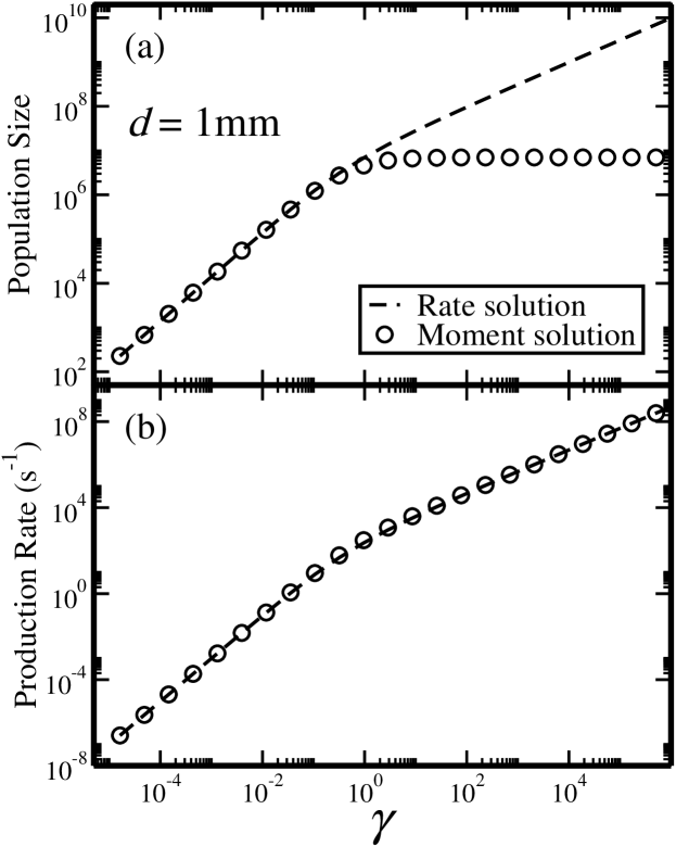
In Fig. 3(a) we show the first moment, , as obtained from the moment equations (circles) vs. , for a very large grain of diameter mm, where . The results are compared with those of the rate equation (dashed line), which under these conditions is accurate. For (second order kinetics) the rate equation and the moment equations coincide. For (first order kinetics) the moment-equation results for the average population size deviate from those of the rate equation. Note that even when , where the moment equations apply, the population size of atoms per grain is very large, much beyond the cutoffs used in the construction of the equations. In Fig. 3(b) we present the production rate of H2 molecules per grain vs. , as obtained from the moment equations (circles). The results are in perfect agreement with those of the rate equations (dashed line) in the regime of first order kinetics as well as in the regime of second order kinetics. These results can be generalized to more complex networks. The analysis becomes more tedious, but the conclusions about the domain of validity of the moment equations remain the same. From a physical perspective, in first order kinetics the reaction is dominant and desorption is suppressed, while in second order kinetics desorption is dominant and the reaction rate is low and diffusion limited.
III Complex Reaction Networks
III.1 The Water-Producing Network
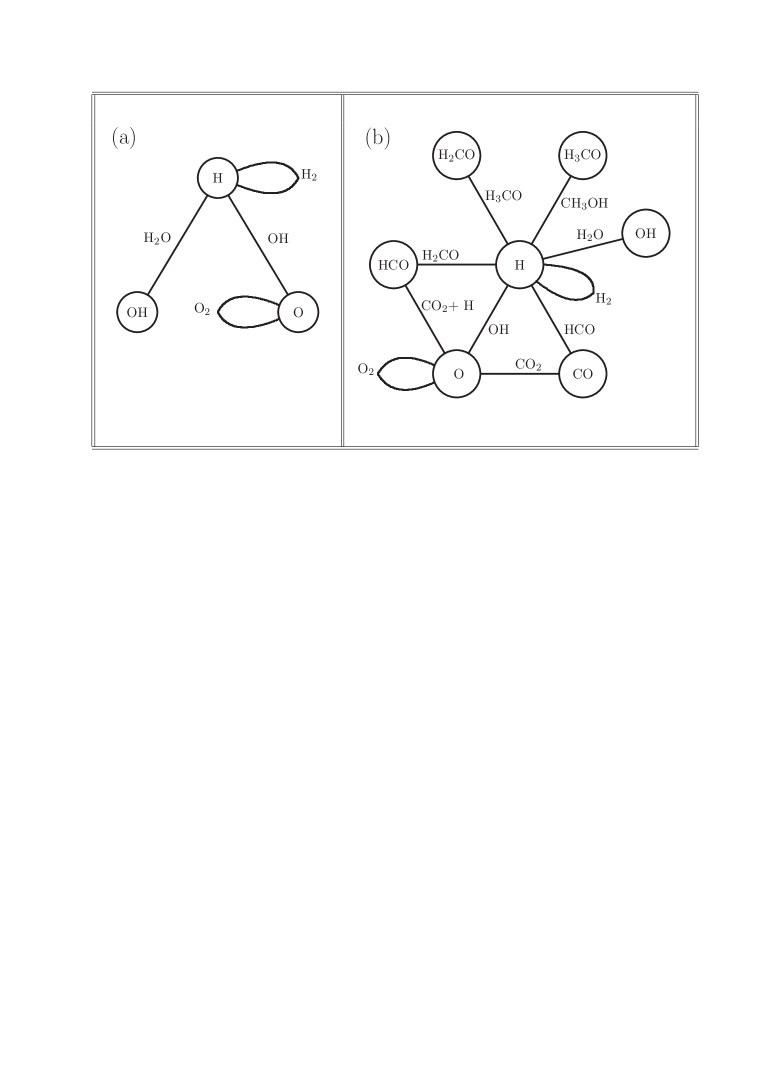
To generalize the analysis beyond the case of a single species, consider a simple chemical network that involves three reactive species: H and O atoms and OH molecules Caselli1998 ; Shalabiea1998 ; Stantcheva2001 . For simplicity we denote the reactive species by H, O, OH, and the resulting non-reactive species by H2, O2, H2O. The reactions that take place in this network include H + O OH (), H + H H2 (), O + O O2 (), and H + OH H2O (). A graph of that network is displayed in Fig. 4(a).
Now, the desorption rates of atomic and molecular species on the grain are given by , where is the activation energy barrier for desorption of species and (K) is the surface temperature. The hopping rate of adsorbed atoms between adjacent sites on the surface is , where is the activation energy barrier for hopping of atoms (or molecules). The sweeping rate will be .
The master equation provides the time derivatives of the probabilities that a randomly chosen grain will have atoms or molecules of the reactive species . It takes the form
| (15) |
The terms in the first sum describe the incoming flux, where (atoms s-1) is the flux per grain of the species . The second sum describes the effect of desorption. The third sum describes the effect of diffusion-mediated reactions between two identical atoms and the last two terms account for reactions between different species. The rate of each reaction is proportional to the number of pairs of atoms of the two species involved, and to the sum of their sweeping rates. The average population size of the species on the grain is , where , and , 2 or 3. The production rate per grain (molecules s-1) of molecules produced by the reaction is given by , or by in case that .
For complex networks with more than one species the truncation of the master equation demands setting upper cutoffs for all the reactive species, , , where is the number of reactive species. The number of coupled equations is then , which grows exponentially with the number of reactive species. This severely limits the applicability of the master equation to interstellar chemistry Stantcheva2002 ; Stantcheva2003 . To reduce the number of equations one tries to use the lowest possible cutoffs under the given conditions. In any case, to enable all reaction processes to take place, the cutoffs must satisfy for species that form homonuclear diatomic molecules (H2, O2, etc.) and for other species.
As in the case of hydrogen recombination, the population sizes and reaction rates are completely determined by all the first moments and selected second moments of the distribution . Therefore, a closed set of equations for the time derivatives of these first and second moments could provide the complete information on the population sizes and reaction rates. For the simple network considered here one needs equations for the time derivatives of the first moments , and of the second moments , , and . We obtain these equations from the master equation using the identity
| (16) |
where are integers. Here we show three of the resulting moment equations:
| (17) | |||||
As expected, the right hand sides of these equations include third order moments for which we have no equations. If we add equations for their time derivatives, they will include fourth order moments, and again will not enable us to close the set of equations. In order to close the set of moment equations we must express the third order moments in terms of the first and second order moments. We recall that in the case of a single reactive specie this was achieved by imposing an extremely restrictive cutoff on the master equation. Generalizing it to our present system we choose the minimal cutoffs that do not terminate any of the reactions taking part in the network. These cutoffs allow at most two atoms or molecules to be adsorbed on the surface at any given time. Furthermore, any two atoms or molecules that reside simultaneously on the surface must belong to species that react with each other. In our network these cutoffs allow only eight non-vanishing probabilities, namely, , , , , , , and . Expressing the third moments, with these cutoffs, leads to the following results:
| (18) |
Using these rules to modify Eqs. (17) one obtains a closed set of the form
| (19) |
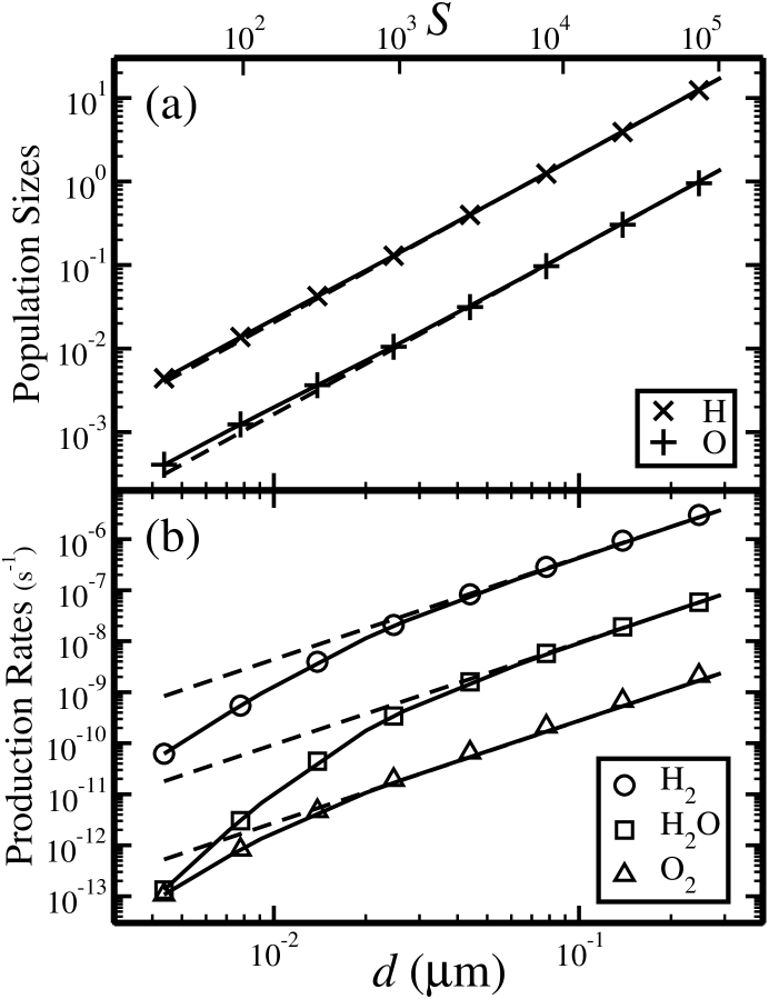
This set of equations is the minimal set required for the system. It includes one equation that accounts for the population size of each reactive specie and one equation that accounts for the reaction rate of each reaction. As in the hydrogen system, the equations were derived using extremely strict cutoffs, that are expected to apply only in the limit of small grains and low flux. Nevertheless, the moment equations are valid well beyond the restrictive cutoffs under which they were derived. In Fig. 5(a) we present the population sizes of H () and O () atoms on a grain vs. grain diameter, obtained from the moment equations. In Fig. 5(b) we show the production rates of H2 (circles), O2 (triangles) and H2O (squares), obtained from the moment equations. The results are in excellent agreement with the master equation and in the limit of large grains they also coincide with the rate equations. The parameters used in the simulations are (atoms s-1), and . The activation energies for diffusion and desorption were taken as , , , , and meV for H, O and OH respectively. The surface temperature of the grain was K. For the species other than H there are no concrete experimental results, and the values reflect the tendency of heavier species to bind more strongly.
The generalization to more complex networks is straightforward. As explained above, the cutoffs imposed on the master equation give rise to a minimal set of non-vanishing probabilities, that allow all the reactions to take place. These non-vanishing probabilities are for the each node, , and for each edge connecting nodes and . A loop connected to the node corresponds to the probability . All other probabilities vanish. In the realm of two-body reactions additional probabilities such as or are never required. Under these restrictions, one can easily show that all the third moments that appear in the moment equations can be expressed in terms of second moments according to Eq. (18).
III.2 The Methanol Network
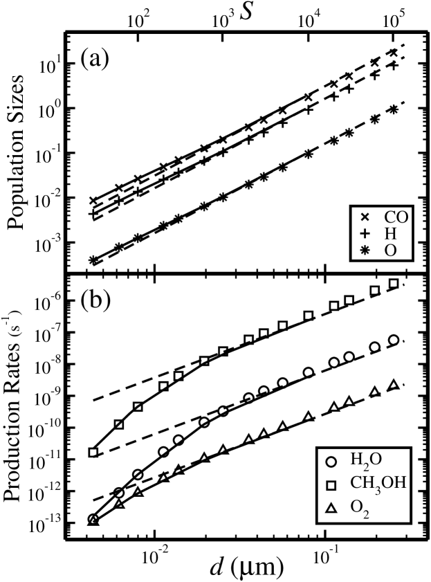
Let us now examine how the moment equation method performs in a more complex network. Recent laboratory experiments provide evidence that methanol in interstellar clouds is formed via reaction networks on dust grains Geppert2006 ; Watanabe2005 . To simulate these networks, consider the case in which a flux of CO molecules is added to the network shown in Fig. 4(a). This gives rise to the network shown in Fig. 4(b), which includes the following sequence of hydrogen addition reactions Stantcheva2002 : H + CO HCO (), H + HCO H2CO (), H + H2CO H3CO () and H + H3CO CH3OH (). Two other reactions that involve oxygen atoms also take place: O + CO CO2 () and O + HCO CO2 + H (). This network was studied before using the multiplane method, which required about a thousand equations compared to about a million equations in the master equation with similar cutoffs. The moment equations include one equation for each species (node in the graph) and one equation for each reaction (edge in the graph), namely, the network shown in Fig. 4(b) requires only 17 equations. We have performed extensive simulations of this network using the moment equations and found that they are in agreement with the master equation results. In Fig. 6(a) we present the population sizes of H (), O () and CO () on a grain vs. grain diameter, as obtained from the moment equations. In Fig. 6(b) we present the results of the moment equations for the formation rates of CH3OH (squares), H2O (circles) and O2 (triangles) and compare them to the master equation (solid line) and the rate equations (dashed lines). As before, the moment equations prove to be consistent with the master equation, and for large grains with the rate equations as well. In the simulations presented here the activation energies for diffusion and desorption of CO, HCO, H2CO and H3CO were taken as , , , , , and , meV, respectively. The flux of CO molecules was taken as .
In complex reaction networks the reduction in the number of equations becomes extremely significant. For each reactive species, (denoted by a node in the graph), there is one equation for the time derivative of the first moment . For each reaction, between species and (represented by an edge), there is one equation for the time derivative of the second moment . The number of equations is thus , where and are the numbers of nodes and edges, respectively. Most reaction networks are sparse, namely the number of edges is of the same order of magnitude as the number of nodes. As a result, the number of moment equations is roughly linearly dependent on the number of species. This is in contrast with the exponential growth of the master equation and the polynomial growth of the multiplane equations Lipshtat2004 .
IV Diagrammatic Construction of the Equations
In the previous Section we described a procedure for the construction of the moment equations, that consists of three steps. In the first step the desired set of moment equations is determined according to the network graph. This set includes one equation for the first moment associated with each species (node) and one equation for the second moment associated with each reaction (edge or loop). In the second step the time derivative of each of these moments is expressed as a suitable linear combination of first, second and third moments. In the third step the equations are brought into a closed form, by expressing all third moments in terms of first and second moments according to Eq. (18). This procedure is suitable for simple networks but becomes difficult to execute as the network complexity increases.
Here we present a simple and highly efficient diagrammatic approach for the construction of the moment equations for any given network. Consider the reaction networks shown in Fig. 4. Each node in the graphs represents one of the reactive species, and each edge stands for a reaction between two species. A loop represents a reaction between two atoms/molecules of the same species. The list of moments that should be included in the moment equations is easily obtained from the graph: (a) For each each node, , there is an equation for the first moment ; (b) For each edge connecting the nodes and there is an equation for the second moment ; (c) for each loop attached to node there is an equation for the second moment .
To derive the moment equations from the graph of a given network, we show how each element in the graph is expressed in the master equation and then translate it into a corresponding term in the moment equations. Consider first the contribution of nodes. Each node represents a species, that may be adsorbed on the surface or desorbed from it. In the master equation, these two processes are described by
To construct the equation for we sum over all the terms of the master equation, according to Eq. (16). The terms above then make the following contribution to the moment equations
| (21) |
In case that the species reacts with itself, one needs to include an equation for . As before, a proper summation over the master equation is performed, but here the contribution of the node will be
| (22) |
If the species reacts with some other species, , it will be necessary to include an equation for . The contribution of the node to this equation is
| (23) |
Note that in the equation for , one should also include the analogous term for the node .
Consider the contribution of edges to the moment equations. Each edge represents a reaction between two different species. In the master equation, the term related to the edge between and is
The contributions of this term to the moment equations appear in all the equations for moments involving either species or species . For example, the contribution to the equation for is
After applying the rules of Eq. (18), this term simplifies to .
In general, each moment equation is obtained by a proper summation over terms of the master equation, using Eq. (16). Each term in the master equation describes a certain process such as adsorption, desorption or reaction. Consider the equations for and . When the summations are carried out, the only non-vanishing contributions are from processes that involve the species . Similarly, consider the equation for . In this case the only non-vanishing contributions are from processes that involve either the species or the species . This gives rise to a dramatic simplification in the construction of the moment equations. In the equation for any desired moment we need to consider only those master equation terms related to the species that appear in that particular moment. In the diagrams, this means including only graph elements that are directly connected to the corresponding nodes. The complete set of translation rules from a given graph element to the corresponding terms in the moment equations is given in Tables 2 - 4.
To demonstrate the construction of the moment equations we reconsider the reaction network shown in Fig. 4(a). First, we identify the relevant moments associated with the nodes, edges and loops in the network graph. In this particular network, the nodes call for , and . The edges call for and . Finally, the two loops in the graph require the inclusion of and . Altogether, there are seven equations. Let us begin with the equation for . This species is represented by a node connected to two edges and one loop. Using our diagrammatic scheme, this equation takes the form
| (26) |
This equation simply consists of all the graph elements related to the species . That diagrammatic sum can be translated, using Table 2, giving rise to the equation
| (27) | |||||
The same diagrammatic equation [Eq. (26)] is used when writing the equation for the time derivative of . However, the translation rules from graph elements to equation terms are different and are given in Table 3. Using these rules we obtain
| (28) | |||||
Next, we construct the moment equation for . This time we need to include some additional graph elements, namely, those related to , so the diagrammatic equation takes the form
| (29) |
This is an equation for a mixed second moment, that should be translated according to Table 4. The resulting equation is
| (30) |
The last equation that we demonstrate explicitly is for the moment . This time the diagrammatic equation will include an additional graph element stating the fact that is produced by a reaction between the other two species in the network. The diagrammatic equation is
| (31) |
which, according to Table 2 translates to
| (32) |
This procedure enables an efficient and straightforward construction of the set of moment equations for any given graph, regardless of its complexity. The construction process can be easily automated into a computer program that receives the network structure as an input and provides the set of equations as an output. This opens the way to efficient stochastic modeling of complex reaction networks of any size.
V Summary
We have presented an efficient method for the stochastic simulation of complex reaction networks. The method is based on moment equations. It accounts correctly for the reaction rates not only for macroscopic populations, where rate equations apply, but also in the limit of low copy numbers where fluctuations dominate. The method exhibits several crucial advantages over existing techniques for stochastic simulations. The number of equations is reduced to the absolute minimum in a stochastic simulation, namely one equation for each reactive species and one equation for each reaction. For any given network the set of moment equations can be constructed easily and efficiently using a diagrammatic approach. The equations are linear, thus, for steady-state conditions they can be easily solved using algebraic methods.
We have demonstrated the method for reactions taking place on dust-grain surfaces in interstellar clouds. We have shown that it applies very well even under the extreme interstellar conditions of low gas density and sub-micron grain sizes. The moment equations can be easily coupled to the rate equation models of interstellar gas-phase chemistry. Therefore, the proposed method is expected to enable the incorporation of grain-surface chemistry into these models.
We expect this method to be useful for the simulation of many other systems that exhibit a related mathematical structure Biham2005 . One such application is for reactions taking place on terrestrial surfaces such as metal catalysts in nanometric systems Suchorski1998 ; Suchorski1999 ; Suchorski2001 ; Johanek2004 ; Pineda2006 ; Liu2002 . Another example is aerosol chemistry in stratospheric clouds, where complex reaction networks involving aerosol particles take place Hanson1994 . The gas density is not nearly as low as in the interstellar clouds. However, the small size of the aerosol particles and the low density of some of the reactive species may require stochastic methods. Another example is genetic networks in cells and bacteria McAdams1997 ; Paulsson2000 ; Lipshtat2006 ; Alon2006 . These networks describe the process of protein synthesis and its regulation. They include the interactions between genes, mRNA’s and proteins. Since some of these components appear in low copy numbers, the simulation of these networks requires stochastic methods.
We thank Azi Lipshtat for helpful discussions. This work was supported by the Israel Science Foundation and the Adler Foundation for Space Research.
References
- (1) N.G. van Kampen, Stochastic Processes in Physics and Chemistry (North-Holland, Amsterdam, 1981).
- (2) I. Oppenheim, K.E. Shuler and G.H. Weiss, Physica A 88, 191 (1977).
- (3) S. Karlin and H.M. Taylor, An Introduction to Stochastic Modeling (Academic Press, San Diego, 1998).
- (4) I. Nasel, Adv. Appl. Probab. 28, 895 (2001).
- (5) D.T. Gillespie, J. Phys. Chem. 81, 2340 (1977).
- (6) M.E.J. Newman and G.T. Barkema, Monte Carlo methods in statistical physics (Clarendon Press, Oxford, 1999).
- (7) D.A. McQuarrie, J. Chem. Phys. 38, 433 (1963).
- (8) D.A. McQuarrie, C.J. Jachimowski and M.E. Russell, J. Chem. Phys. 40, 2914 (1964).
- (9) C.W. Gardiner, Handbook of Stochastic Methods (Springer, Berlin, 1985).
- (10) M. Assaf and B. Meerson, Phys. Rev. Lett. 97, 200602 (2006).
- (11) M. Assaf and B. Meerson, Phys. Rev. E 75, 031122 (2007).
- (12) N.J.B. Green, T. Toniazzo, M.J. Pilling, D.P. Ruffle, N. Bell and T.W. Hartquist, Astron. Astrophys. 375, 1111 (2001).
- (13) O. Biham and A. Lipshtat, Phys. Rev. E 66, 056103 (2002).
- (14) E.W. Montroll, J. Chem. Phys. 14, 202 (1946).
- (15) A. Kolmogorov, Mathem. Annalen 104, 415 (1931).
- (16) A. Lipshtat, O. Biham, Phys. Rev. Lett. 93, 170601 (2004).
- (17) B. Barzel and O. Biham, Astrophys. J. 658, L37 (2007).
- (18) Yu. Suchorski, R. Imbihl and V.K. Medvedev, Surf. Sci. 401, 392 (1998).
- (19) Yu. Suchorski, J. Beben, E.W. James, J.W. Evans and R. Imbihl, Phys. Rev. Lett. 82, 9 (1999).
- (20) Yu. Suchorski, J. Beben, R. Imbihl, E.W. James, D.-J. Liu and J.W. Evans, Phys. Rev. B 63, 165417 (2001).
- (21) V. Johanek, M. Laurin, A.W. Grant, B. Kasemo, C.R. Henry and J, Libuda, Science 304, 1639 (2004).
- (22) M. Pineda, R. Imbihl, L. Schimansky-Geier and Ch. Zülicke, J. Chem. Phys. 124, 044701 (2006).
- (23) D.-J. Liu and J.W. Evans, J. Chem. Phys. 117, 15 (2002).
- (24) L. Spitzer, Physical Processes in the Interstellar Medium (Wiley, New York, 1978).
- (25) T.W. Hartquist and D.A. Williams, The chemically controlled cosmos (Cambridge University Press, Cambridge, UK, 1995).
- (26) T.I. Hasegawa and E. Herbst and C.M. Leung, Astrophys. J. Supp. 82, 167 (1992).
- (27) E. Herbst, Annu. Rev. Phys. Chem. 46, 27 (1995).
- (28) R.J. Gould and E.E. Salpeter, Astrophys. J. 138, 393 (1963).
- (29) D. Hollenbach and E.E. Salpeter, J. Chem. Phys. 53, 79 (1970).
- (30) D. Hollenbach and E.E. Salpeter, Astrophys. J. 163, 155 (1971).
- (31) D. Hollenbach, M.W. Werner and E.E. Salpeter, Astrophys. J. 163, 165 (1971).
- (32) E. Herbst, J. Phys. Chem. 109, 4017 (2005).
- (33) K. Hiraoka, T. Miyagoshi,T. Takayama, K. Yamamoto and Y. Kihara, Astrophys. J. 498, 710 (1998).
- (34) H. Hidaka, N. Watanabe, T. Shiraki, A. Nagaoka and A. Kouchi, Astrophys. J. 614, 1124 (2004).
- (35) Geppert, W.D., Hamberg, M., Thomas, R.D., Österdahl, F., Hellberg, F., Zhaunerchyk, V., Ehlerding, A., Millar, T.J., Roberrts, H., Semaniak, J., af Ugglas, M., Källberg, A., Simonsson, A., Kaminska, M. & Lrsson, M., Faraday Discussions 133: Chemical Evolution of the Universe, p. 177 (2006).
- (36) N. Watanabe, in IAU Symposium 231, Astrochemistry: Recent Successes and Current Challenges, edited by D.C. Lis, G.A. Blake and E. Herbst (Cambridge University Press, Cambridge, UK, 2005), p. 415.
- (37) A.G.G.M. Tielens and W. Hagen, Astron. Astrophys. 114, 245 (1982).
- (38) S.B. Charnley, A.G.G.M. Tielens and S.D. Rodgers, Astrophys. J. 482, L203 (1997).
- (39) P. Caselli, T.I. Hasegawa and E. Herbst, Astrophys. J. 495, 309 (1998).
- (40) O.M. Shalabiea, P. Caselli and E. Herbst, Astrophys. J. 502, 652 (1998).
- (41) O. Biham, I. Furman, V. Pirronello and G. Vidali, Astrophys. J. 553, 595 (2001).
- (42) S.B. Charnley, Astrophys. J. 562, L99 (2001).
- (43) T. Stantcheva, V.I. Shematovich and E. Herbst, Astron. Astrophys. 391, 1069 (2002).
- (44) T. Stantcheva and E. Herbst, Mon. Not. R. Astron. Soc. 340, 983 (2003).
- (45) V. Pirronello, C. Liu, L. Shen and G. Vidali, Astrophys. J. 475, L69 (1997).
- (46) V. Pirronello, O. Biham, C. Liu, L. Shen and G. Vidali, Astrophys. J. 483, L131 (1997).
- (47) J.E. Roser, G. Manicò, V. Pirronello and G. Vidali, Astrophys. J. 581, 276 (2002).
- (48) L. Hornekaer, A. Baurichter, V.V. Petrunin, D. Field and A.C. Luntz, Science 302, 1943 (2003).
- (49) L. Hornekaer, A. Baurichter, V.V. Petrunin, A.C. Luntz, B.D. Kay and A. Al-Halabi, J. Chem. Phys. 122, 124701 (2005).
- (50) G. Vidali, J. Roser, V. Pirronello, H.B. Perets and O. Biham, Journal of Physics: Conference Series 6, 36 (2005).
- (51) L. Amiaud, J.H. Fillion, S. Baouche, F. Dulieu, A. Momeni and J.L. Lemaire, J. Chem. Phys. 124, 094702 (2006).
- (52) N. Katz, I. Furman, O. Biham, V. Pirronello and G. Vidali, Astrophys. J. 522, 305 (1999).
- (53) H.B. Perets, O. Biham, V. Pirronello, J.E. Roser, S. Swords, G. Manico and G. Vidali, Astrophys. J. 627, 850 (2005).
- (54) J. Krug, Phys. Rev. E 67, 065012 (2003).
- (55) I. Lohmar and J. Krug, Mon. Not. R. Astron. Soc. 370, 1025 (2006).
- (56) O. Biham, I. Furman, N. Katz, V. Pirronello and G. Vidali, Mon. Not. R. Astron. Soc. 296, 869 (1998).
- (57) A. Lipshtat, O. Biham, Astron. Astrophys. 400, 585 (2003).
- (58) D.A. McQuarrie, J. Appl. Prob. 4, 413 (1967).
- (59) C.A. Gómez-Uribe and G.C. Verghese, J. Chem. Phys. 126, 024109 (2007).
- (60) T. Stantcheva, P. Caselli and E. Herbst, Astron. Astrophys. 375, 673 (2001).
- (61) O. Biham, J. Krug, A. Lipshtat and T. Michely, Small 1, 502 (2005).
- (62) D.R. Hanson, A.R. Ravishankara and S. Solomon, J. Geophys. Res. 99, 3615 (1994).
- (63) H.H. McAdams and A. Arkin, 94, 814 (1997).
- (64) J. Paulsson and M. Ehrenberg, Phys. Rev. Lett. 84, 5447 (2000).
- (65) A. Lipshtat, A. Loinger, N.Q. Balaban and O. Biham, Phys. Rev. Lett. 96, 188101 (2006).
- (66) U. Alon, An Introduction to Systems Biology: Design Principles of Biological Circuits (Chapman & Hall, London, 2006).
| The Validity of the Moment Equations | |||
| Small Grain | Large Grain | ||
| First order | |||
| Second order | |||
| Graph Elements Translation for the Equation | ||
|---|---|---|
| Graph Element | Equation Term | Reduced Equation Term |
| () | () | |
| () | () | |
| Graph Elements Translation for the Equation | ||
| Graph Element | Equation Term | Reduced Equation Term |
| ( | ||
| ) | () | |
| ( | ||
| ) | ||
| ( | ||
| ) | ||
| ( | ||
| ) | () | |
| Graph Elements Translation for the Equation | ||
| Graph Element | Equation Term | Reduced Equation Term |
| ( ) | () | |
| ( | ||
| ) | ||
| ( ) | () | |
| ( | ||
| ) | ||
| ( ) | (( | |
| )) | ||