Evaluation of the Multiplane Method for Efficient
Simulations of Reaction Networks

Abstract

Reaction networks in the bulk and on surfaces are widespread in physical, chemical and biological systems. In macroscopic systems, which include large populations of reactive species, stochastic fluctuations are negligible and the reaction rates can be evaluated using rate equations. However, many physical systems are partitioned into microscopic domains, where the number of molecules in each domain is small and fluctuations are strong. Under these conditions, the simulation of reaction networks requires stochastic methods such as direct integration of the master equation. However, direct integration of the master equation is infeasible for complex networks, because the number of equations proliferates as the number of reactive species increases. Recently, the multiplane method, which provides a dramatic reduction in the number of equations, was introduced [A. Lipshtat and O. Biham, Phys. Rev. Lett. 93, 170601 (2004)]. The reduction is achieved by breaking the network into a set of maximal fully connected sub-networks (maximal cliques). Lower-dimensional master equations are constructed for the marginal probability distributions associated with the cliques, with suitable couplings between them. In this paper we test the multiplane method and examine its applicability. We show that the method is accurate in the limit of small domains, where fluctuations are strong. It thus provides an efficient framework for the stochastic simulation of complex reaction networks with strong fluctuations, for which rate equations fail and direct integration of the master equation is infeasible. The method also applies in the case of large domains, where it converges to the rate equation results.

I Introduction

Reaction networks commonly appear in physical, chemical and biological systems, where reactions may take place in the bulk or on a surface. When the surface or bulk systems are macroscopic, the populations of reactive species are typically large and the law of large numbers applies. Thus, fluctuations in the concentrations of the reactants and in the reaction rates become negligible. As a result, these reaction networks can be analyzed using rate equation models, which account for the average concentrations and ignore fluctuations.

In some cases, the system is partitioned into small domains, such that the reactants cannot diffuse between them. The populations of reactive species in each domain become small and their fluctuations cannot be ignored. As a consequence, rate equations fail and the simulation of these reactions requires stochastic methods such as direct integration of the master equation vanKampen1981 . The master equation takes into account the discrete nature of the reactants as well as the fluctuations. It is expressed in terms of the probabilities of having a given set of population sizes of the reactive species in a given domain. In certain cases, such as radioactive decay, an analytical solution based on generating functions is available McQuarrie1967 . In other cases, numerical methods are required. For simple reaction networks that involve few reactive species, numerical integration of the master equation is useful and efficient Biham2001 ; Green2001 ; Biham2002 . However, as the number of reactive species increases, the number of variables in the master equation quickly proliferates Stantcheva2002 ; Stantcheva2003 , making the direct integraion infeasible.

Here we focus on networks in which reactions take place between pairs of species, and the reaction products may be reactive or non-reactive. Such networks may be described by graphs: each reactive species is represented by a node; the reaction between a pair of species is represented by an edge that connects the corresponding nodes. Typically, these networks are sparse, namely most pairs of species do not react with each other. For such sparse networks, the recently introduced multiplane method provides a dramatic reduction in the number of equations Lipshtat2004 . The method is based on breaking the network into a set of maximal fully connected subnetworks (maximal cliques). It involves an approximation, in which the correlations between pairs of species that react with each other are maintained, while the correlations between non-reacting pairs are neglected. The result is a set of lower dimensional master equations, one for each clique, with suitable couplings between them. For sparse networks, the cliques are typically small and mostly consist of two or three nodes. This method thus enables the simulation of large networks much beyond the point where the master equation becomes infeasible.

The multiplane method has already been used in the simulation of complex chemical networks on dust grains in interstellar clouds Lipshtat2004 , where rate equations fail Tielens1982 ; Charnley1997 ; Caselli1998 ; Shalabiea1998 , while direct integration of the master equation is impractical Stantcheva2002 ; Stantcheva2003 . The multiplane method is also required for the simulation of genetic networks in cells, where the master equation Paulsson2000 ; Paulsson2000b ; Paulsson2004 and Monte Carlo simulations Gillespie1977 ; Mcadams1997 ; Mcadams1999 are not applicable for large networks.

In this paper we analyze the multiplane method and examine its validity. This is done by comparing the results with the complete master equation. The comparison is done both for the probability distributions and for the first and second moments, which represent the population sizes of reactants and reaction rates, respectively. It is shown that the multiplane method provides accurate results for both the population sizes and reaction rates. For concreteness, we use below the terminology of surface reactions. In this context, the small domains are taken to be dust grains (assumed to be spherical, for simplicity), and the reactants are atoms or molecules that enter the system as incoming flux from the surrounding gas phase (below we use the words atoms and molecules interchangeably). The reactants and reaction products leave the system by thermal desorption. The reactions that take place on a grain are driven by diffusion of reactants on its surface until they encounter each other and react. In spite of this specific terminology, the multiplane method can be adapted to other contexts, such as reactions in a solution, protein interactions in a living cell and birth-death processes in population dynamics. Here we focus on the calculation of steady-state solutions and thus do not expand on birth-death processes which may exhibit absorbing states.

The paper is organized as follows. In Sec. II we briefly review the rate equation and master equation methods, presenting them for a simple reaction network. In Sec. III we describe the multiplane method. In Sec. IV we test the performance of the multiplane method. An analysis of the method in the limits of small and large grains is presented in Sec. V. In Sec. VI we show how to apply the method to more complex networks. In Sec. VII we briefly describe its applications in interstellar chemistry and in genetic networks. The main findings are summarized and discussed in Sec. VIII.

II The Rate Equations and the Master Equation

Consider a small grain, exposed to fluxes of three different atomic species, denoted by $X_{1}$, $X_{2}$ and $X_{3}$. The adsorbed atoms on the grain reside in adsorption sites. The number of sites, $S$, is proportional to the surface area of the grain. The incoming flux of $X_{i}$, $i=1,2,3$, is given by $f_{i}$ (s^-1) atoms per site. Thus, the flux of atoms per grain is $F_{i}=f_{i}S$ (s^-1). The adsorbed atoms may desorb due to thermal excitations. The desorption rate of the $X_{i}$ species from the grain is denoted by $W_{i}$ (s^-1). While residing on the grain, the atoms diffuse on the surface via hopping between adjacent sites. The hopping rate of $X_{i}$ atoms is given by $a_{i}$ (hops s^-1). It is convenient to define the sweeping rate $A_{i}=a_{i}/S$, which is approximately the inverse of the time it takes an adsorbed $X_{i}$ atom to visit nearly all the adsorption sites on the grain surface Lipshtat2002 . A more accurate expression for $A_{i}$ in the case of spherical grains appears in Ref. Lohmar2006 , where it is shown to be reduced by a logarithmic factor.

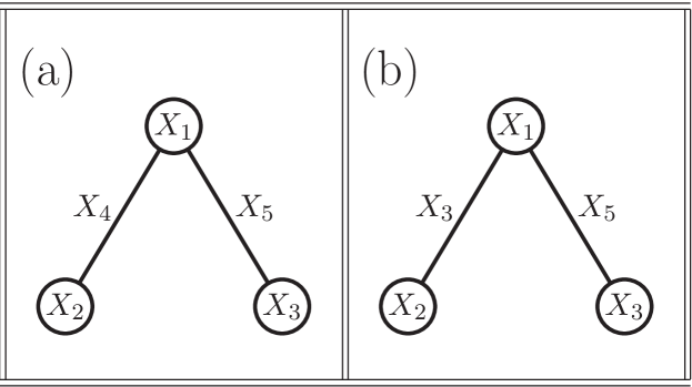
Figure 1: Graphic representations of two reaction networks that involve three reactive species. The nodes represent reactive species and the edges represent reactions between pairs of species. The reaction products are specified near the edges. In these networks there are two cliques: one consists of $X_{1}$ and $X_{2}$ and the other consists of $X_{1}$ and $X_{3}$. (a) The reaction products, $X_{4}$ and $X_{5}$ are non-reactive; (b) The product of the reaction between $X_{1}$ and $X_{2}$ is the reactive specie $X_{3}$.

The diffusion process enables adsorbed atoms to encounter each other and react. Here we consider a simple reaction network that includes the reactions $X_{1}+X_{2}\longrightarrow X_{4}$ and $X_{1}+X_{3}\longrightarrow X_{5}$, where the $X_{4}$ and $X_{5}$ molecules are the reaction products. The graph that illustrates this network is shown in Fig. 1(a).

II.1 The Rate Equations

The rate equations that describe the network of Fig. 1(a). take the form

$$\frac{d\langle N_{1}\rangle}{dt} = F_{1}-W_{1}\langle N_{1}\rangle-(A_{1}+A_{2})\langle N_{1}\rangle\langle N_{2}\rangle-(A_{1}+A_{3})\langle N_{1}\rangle\langle N_{3}\rangle$$

$$\frac{d\langle N_{2}\rangle}{dt} = F_{2}-W_{2}\langle N_{2}\rangle-(A_{1}+A_{2})\langle N_{1}\rangle\langle N_{2}\rangle$$

$$\frac{d\langle N_{3}\rangle}{dt} = F_{3}-W_{3}\langle N_{3}\rangle-(A_{1}+A_{3})\langle N_{1}\rangle\langle N_{3}\rangle,$$ (1)

where $\langle N_{i}\rangle$ is the average population size of $X_{i}$ atoms on a grain. The first terms on the right hand side of Eq. (1) represent the incoming fluxes of $X_{i}$ atoms. The second terms represent the desorption of $X_{i}$ atoms, which is proportional to the $X_{i}$ population on the grain. The remaining terms account for the reactions between adsorbed atoms. The production rates of $X_{4}$ and $X_{5}$ molecules per grain (in units of s^-1) are given by $R_{4}=(A_{1}+A_{2})\langle N_{1}\rangle\langle N_{2}\rangle$ and $R_{5}=(A_{1}+A_{3})\langle N_{1}\rangle\langle N_{3}\rangle$. For simplicity, we assume that non-reactive product species desorb into the gas phase immediately upon formation.

For large grains, Eqs. (1) account correctly for the reaction rates. However, in the limit of small grains, some of the average population sizes, $\langle N_{i}\rangle$, may become small. In this case the discrete nature of the adsorbed atoms and molecules becomes important and the fluctuations cannot be ignored. As a result, the reaction rates obtained from the rate equations (1) are incorrect and stochastic methods are needed.

We also consider a related network, shown in Fig. 1(b), in which $X_{3}$ is the product of the reaction between $X_{1}$ and $X_{2}$ (namely, $X_{3}$ and $X_{4}$ are the same species). The rate equations that describe this system are the same as in Eq. (1) except that in the third equation one needs to add the term $(A_{1}+A_{3})\langle N_{1}\rangle\langle N_{3}\rangle$. The production rate of $X_{5}$ is still given by $R_{5}$ defined above.

II.2 The Master Equation

The dynamical variables of the master equation are the probabilities $P(n_{1},n_{2},n_{3})$ of having a population of $n_{i}$ atoms of species $X_{i}$ on the grain. It takes the form

$$\dot{P}(n_{1},n_{2},n_{3}) = \sum_{i=1}^{3}{F_{i}[P(\dots,n_{i}-1,\dots)-P(n_{1},n_{2},n_{3})]}$$

$$+ \sum_{i=1}^{3}{W_{i}[(n_{i}+1)P(\dots,n_{i}+1,\dots)-n_{i}P(n_{1},n_{2},n_{3})]}$$

$$+ (A_{1}+A_{2})[(n_{1}+1)(n_{2}+1)P(n_{1}+1,n_{2}+1,n_{3})-n_{1}n_{2}P(n_{1},n_{2},n_{3})]$$

$$+ (A_{1}+A_{3})[(n_{1}+1)(n_{3}+1)P(n_{1}+1,n_{2},n_{3}+1)-n_{1}n_{3}P(n_{1},n_{2},n_{3})],$$

where $n_{i}=0,1,2,\dots$. The first term in Eq. (II.2) describes the effect of the incoming flux. The probability $P(\dots,n_{i},\dots)$ increases when an $X_{i}$ atom is adsorbed on a grain that already has $n_{i}-1$ adsorbed $X_{i}$ atoms. This probability decreases when an $X_{i}$ atom is adsorbed on a grain that includes $n_{i}$ atoms of species $X_{i}$. The second term accounts for the desorption process. The third and fourth terms describe the reactions that take place on the grain.

In numerical simulations the master equation is truncated in order to keep the number of equations finite. A convenient way to achieve this is to assign upper cutoffs on the population sizes of the reactive species, $n_{i}^{\rm max}$, $i=1,\dots,J$, where $J$ is the number of reactive species.

In the network of Fig. 1(a), the average population size of $X_{i}$ on a grain is given by the first moment

$$\langle N_{i}\rangle=\sum_{n_{1}=0}^{n_{1}^{\rm max}}\sum_{n_{2}=0}^{n_{3}^{\rm max}}\sum_{n_{3}=0}^{n_{3}^{\rm max}}n_{i}P(n_{1},n_{2},n_{3}).$$ (3)

The production rates per grain of $X_{4}$ and $X_{5}$ molecules can be obtained from the mixed second moments of $P(n_{1},n_{2},n_{3})$, according to $R_{4}=(A_{1}+A_{2})\langle N_{1}N_{2}\rangle$ and $R_{5}=(A_{1}+A_{3})\langle N_{1}N_{3}\rangle$, where

$$\langle N_{i}N_{j}\rangle=\sum_{n_{1}=0}^{n_{1}^{\rm max}}\sum_{n_{2}=0}^{n_{3}^{\rm max}}\sum_{n_{3}=0}^{n_{3}^{\rm max}}n_{i}n_{j}P(n_{1},n_{2},n_{3}).$$ (4)

In a network of $J$ reactive species, the number of equations to be solved is

$$N_{E}=\prod_{i=1}^{J}(n_{i}^{\max}+1).$$ (5)

The truncated master equation is valid if the probability to have a population larger than the assigned cutoff is negligible. Note that $N_{E}$ grows exponentially with the number of reactive species. This limits the applicability of the master equation to simple networks, making it impractical in the case of complex networks which involve many reactive species Stantcheva2002 ; Stantcheva2003 .

III The Multiplane Method

The recently introduced multiplane method provides a dramatic reduction in the number of equations Lipshtat2004 . It thus enables efficient simulations of complex reaction networks. Below we describe the method using the network of Fig. 1(a). Note that in this network the species $X_{1}$ participates in both reactions. Since the species $X_{2}$ and $X_{3}$ do not react with each other, one may assume that for a given population size of $X_{1}$, their population sizes are almost conditionally independent. Under this assumption, the probability distribution of the population sizes can be approximated by Lipshtat2004

$$P(n_{1},n_{2},n_{3})=P(n_{1})P(n_{2}|n_{1})P(n_{3}|n_{1}),$$ (6)

where $P(n_{i}|n_{1})$ is the conditional probability that there will be $n_{i}$ atoms of species $X_{i}$ given that there are $n_{1}$ atoms of species $X_{1}$ on the grain.

In order to derive the multiplane equations, we first insert Eq. (6) into the master Eq. (II.2), and trace over the population size of $X_{3}$. Using the fact that $\sum_{n_{3}}{P(n_{3}|n_{1})}=1$ and that $\sum_{n_{3}}{\dot{P}(n_{3}|n_{1})}=0$, one obtains

$$\dot{P}(n_{1},n_{2}) = F_{1}[P(n_{1}-1,n_{2})-P(n_{1},n_{2})]+F_{2}[P(n_{1},n_{2}-1)-P(n_{1},n_{2})]$$ (7)

$$+ W_{1}[(n_{1}+1)P(n_{1}+1,n_{2})-n_{1}P(n_{1},n_{2})]$$

$$+ W_{2}[(n_{2}+1)P(n_{1},n_{2}+1)-n_{1}P(n_{1},n_{2})]$$

$$+ (A_{1}+A_{2})[(n_{1}+1)(n_{2}+1)P(n_{1}+1,n_{2}+1)-n_{1}n_{2}P(n_{1},n_{2})]$$

$$+ (A_{1}+A_{3})[(n_{1}+1)\langle N_{3}\rangle_{n_{1}+1}P(n_{1}+1,n_{2})-n_{1}\langle N_{3}\rangle_{n_{1}}P(n_{1},n_{2})],$$

where $\langle N_{3}\rangle_{n_{1}}=\sum_{n_{3}}{n_{3}P(n_{3}|n_{1})}$. A similar procedure, tracing over the population size of $X_{2}$, leads to the equation

$$\dot{P}(n_{1},n_{3}) = F_{1}[P(n_{1}-1,n_{3})-P(n_{1},n_{3})]+F_{3}[P(n_{1},n_{3}-1)-P(n_{1},n_{3})]$$ (8)

$$+ W_{1}[(n_{1}+1)P(n_{1}+1,n_{3})-n_{1}P(n_{1},n_{3})]$$

$$+ W_{3}[(n_{3}+1)P(n_{1},n_{3}+1)-n_{1}P(n_{1},n_{3})]$$

$$+ (A_{1}+A_{3})[(n_{1}+1)(n_{3}+1)P(n_{1}+1,n_{3}+1)-n_{1}n_{3}P(n_{1},n_{3})]$$

$$+ (A_{1}+A_{2})[(n_{1}+1)\langle N_{2}\rangle_{n_{1}+1}P(n_{1}+1,n_{3})-n_{1}\langle N_{2}\rangle_{n_{1}}P(n_{1},n_{3})].$$

These are, in fact, two master equations, one for $P(n_{1},n_{2})$ and the other for $P(n_{1},n_{3})$. These two master equations are coupled through the conditional averages $\langle N_{j}\rangle_{n_{1}}$ where $j=2,3$. The conditional average, which is evaluated in each one of these master equations is then used, essentially as a rate constant, in the other master equation. The multiplane equations are solved by direct numerical integration using standard steppers such as Runge-Kutta. At each time step, the probability distributions $P(n_{1},n_{2})$ and $P(n_{1},n_{3})$ are updated. The conditional averages $\langle N_{j}\rangle_{n_{1}}$ are then evaluated and used in the next time step.

The number of equations is significantly reduced as we replace the three-dimensional set of equations for $P(n_{1},n_{2},n_{3})$ by two-dimensional sets for $P(n_{1},n_{2})$, and $P(n_{1},n_{3})$. The number of equations in the three-dimensional set is given by Eq. (5) with $J=3$. The number of equations in each one of the two dimensional sets is $(n_{1}^{\max}+1)(n_{i}^{\max}+1)$, $i=2,3$.

The multiplane method enables one to calculate the average population sizes $\langle N_{i}\rangle$ of all the species, as well as the reaction rates, expressed in terms of the second moments $\langle N_{i}N_{j}\rangle$. Consider, for example, the population size $\langle N_{1}\rangle$ of the $X_{1}$ species. It can be expressed in two ways, namely

$$\langle N_{1}\rangle=\sum_{n_{1}=0}^{n_{1}^{\rm max}}{\sum_{n_{i}=0}^{n_{i}^{\rm max}}{n_{1}P(n_{1},n_{i})}}$$ (9)

where $i=2$ or $3$. In the first case $\langle N_{i}\rangle$ is evaluated from $P(n_{1},n_{2})$, and in the second case it is evaluated from $P(n_{1},n_{3})$. A nice property of the multiplane method is that the results are identical, as can be seen from Eq. (6). The difference is merely in the order in which $N_{2}$ and $N_{3}$ are traced out. The multiplane method also provides the reaction rates. For example, the production rate of the $X_{4}$ species [Fig. 1(a)] is given by

$$R_{4}=(A_{1}+A_{2})\sum_{n_{1}=0}^{n_{1}^{\rm max}}\sum_{n_{2}=0}^{n_{2}^{\rm max}}n_{1}n_{2}P(n_{1},n_{2}).$$ (10)

Note that in the derivation of the multiplane equations, certain dependencies were neglected. Still, the dependence between all pairs of species that react with each other are maintained through the conditional averages, $\langle N_{i}\rangle_{n_{1}}$. These conditional averages are essential in order to maintain the desired correlations. If the conditional moments $\langle N_{i}\rangle_{n_{1}}$, in the multiplane equations (7) and (8), are replaced by $\langle N_{i}\rangle$ for $i=2,3$, these equations are reduced, by proper summations, to the rate equations (1). In this case all the correlations are lost.

IV Simulations and Results

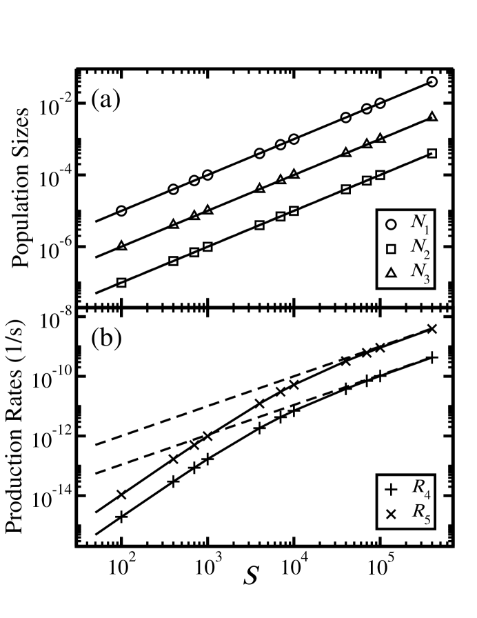
Figure 2: (a) The population sizes of the $X_{1}$ (circles), $X_{2}$ (triangles) and $X_{3}$ (squares) species per grain vs. the number of adsorption sites, $S$, on the grain, obtained from the multiplane equations, for the network shown in Fig. 1(a). The results are in perfect agreement with the master equation (solid lines) and the rate equations (dashed lines); (b) The production rates of $X_{4}$ (+) and $X_{5}$ ($\times$) molecules per grain vs. $S$, obtained from the multiplane equations. The results are in perfect agreement with the master equation (solid lines). For small grains, the rate equation results (dashed lines) for the reaction rates exhibit large deviations. Here, $X_{1}$ is the dominant species.

To examine the multiplane method we have performed simulations of the reaction networks shown in Fig. 1. The results were compared to those obtained from the complete master equation. In Fig. 2(a) we present the average population sizes of the $X_{1}$ (circles), $X_{2}$ (squares) and $X_{3}$ (triangles) species on a grain vs. the number of adsorption sites, $S$, for the network of Fig. 1(a), obtained from the multiplane equations under steady state conditions. In the simulations throughout the paper, we chose to use the parameters $W_{1}=10^{-3}$, $a_{1}=10$, $W_{2}=10^{-3}$, $a_{2}=1$, $W_{3}=10^{-5}$, and $a_{3}=10^{-1}$ (s^-1). This choice reflects the mobilities and desorption rates in the network of H, O and OH that appears in interstellar grain chemistry Stantcheva2001 . The production rates of $X_{4}$ ($+$) and $X_{5}$ ($\times$) molecules on a grain, vs. $S$, obtained from the multiplane equations, are shown in Fig. 2(b). The results are in excellent agreement with the master equation (solid lines). The rate equations (dashed lines) provide accurate results for large grains, but for small grains they show significant deviations. We have preformed extensive simulations of this system, using a wide range of parameters, and found that the consistency of the multiplane method and the complete master equation is always maintained. In the simulations presented above the fluxes were $F_{1}=10^{-8}S$, and $F_{2}=F_{3}=0.01F_{1}$.

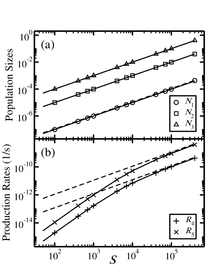
Figure 3: The population sizes (a) and the production rates (b) per grain vs. $S$ for the network of Fig. 1(a). The multiplane results (symbols) are in perfect agreement with the master equation (solid lines). The rate equation results (dashed lines) deviate significantly for small grains. Here the species $X_{1}$ is dominated by $X_{2}$ and $X_{3}$.

Note that with the parameters specified above, the incoming flux of $X_{1}$ atoms is much larger than the fluxes of $X_{2}$ and $X_{3}$. It is often the case in chemical networks that there exists a dominant species, which is more abundant and more reactive than the other species (such as hydrogen in interstellar grain chemistry). One could speculate that the dominance of $X_{1}$ is the reason for the remarkable agreement between the multiplane results and the master equation results. In order to show that this is not the case, and that the multiplane equations are generically applicable, we examine some other parameters. In particular, we consider the case in which the flux of $X_{1}$ is much lower than the fluxes of $X_{2}$ and $X_{3}$, namely $F_{2}=F_{3}=10^{-8}$ and $F_{1}=0.01F_{2}$. The population sizes and reaction rates obtained for this choice of fluxes are shown in Fig. 3(a) and (b), respectively. Clearly, the excellent agreement between the multiplane method and the master equation is maintained in this case as well as in all other sets of parameters that we have examined.

It turns out that the multiplane method applies even when one of the species in one clique is a product of a reaction that is included in another clique. To demonstrate this fact we consider the network of Fig. 1(b) in which $X_{3}$ is the product of the reaction between $X_{1}$ and $X_{2}$. This feature may give rise to some sort of correlation between the population sizes of $X_{2}$ and $X_{3}$. The question is whether such correlations may reduce the applicability of the multiplane method.

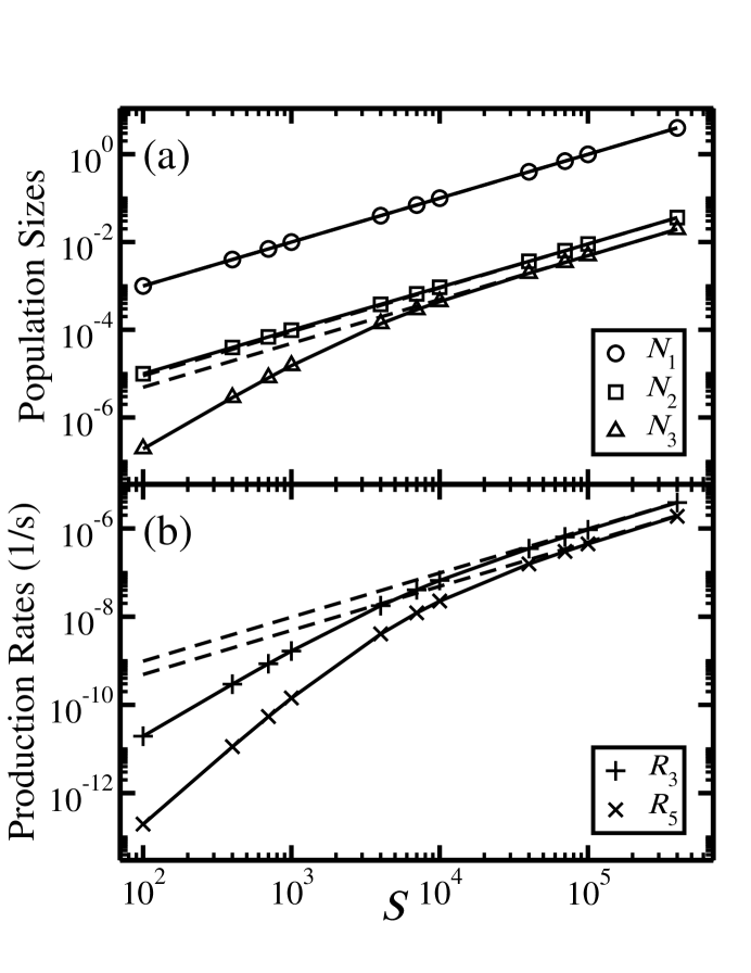
Figure 4: The population sizes (a) and the production rates (b) per grain vs. $S$, for the network of Fig. 1(b) in which $X_{3}$ is the reaction product of $X_{1}$ and $X_{2}$. The multiplane results (symbols) are in perfect agreement with the master equation (solid lines). The rate equations (dashed lines) are also shown.

The multiplane equations describing the network of Fig. 1(b) are the same as Eqs. (7) and (8), except that in the last term of the second equation, $P(n_{1}+1,n_{3})$ is replaced by $P(n_{1}+1,n_{3}-1)$. In Fig 4(a) we present the population sizes of the $X_{1}$ (circles), $X_{2}$ (triangles) and $X_{3}$ (squares) species on a grain vs. $S$ under steady state conditions, obtained from the multiplane method for the network of Fig. 1(b). The production rates of the $X_{3}$ (+) and $X_{5}$ ($\times$) species are shown in Fig. 4(b) . Even in this case, the multiplane results are in perfect agreement with the master equation (solid lines). The rate equations (dashed lines) are accurate for large grains but deviate for small grains. Here we chose $F_{1}=10^{-8}$, $F_{2}=0.01F_{1}$ and $F_{3}=0$, namely $X_{3}$ molecules are not accreted from the gas phase, and are produced only on the grain.

Figs. 2 - 4 demonstrate the usefulness of the multiplane method for the simulation of reaction networks on small grains. In particular, it is shown that the multiplane equations provide accurate results for the population sizes of reactants, given by the first moments $\langle N_{i}\rangle$, $i=1,2,3$, and for the reaction rates, expressed in terms of the second moments, $\langle N_{1}N_{2}\rangle$ and $\langle N_{1}N_{3}\rangle$.

The multiplane method only includes the marginal probability distributions, $P(n_{1},n_{2})$ and $P(n_{1},n_{3})$. However, using Eq. (6) one can construct an approximation of the complete probability distribution, $P(n_{1},n_{2},n_{3})$. This approximation takes the form

$$P_{\rm MP}(n_{1},n_{2},n_{3})=\frac{P(n_{1},n_{2})P(n_{1},n_{3})}{P(n_{1})},$$ (11)

where the marginal probability distributions $P(n_{1},n_{2})$, $P(n_{1},n_{3})$ and $P(n_{1})$ on the right hand side are those obtained from the multiplane method. In order to examine the accuracy of this approximation, we introduce the deviation distance,

$$\Delta=\sum_{n_{1},n_{2},n_{3}}{\left|P(n_{1},n_{2},n_{3})-P_{\rm MP}(n_{1},n_{2},n_{3})\right|},$$ (12)

which is evaluated under steady-state conditions of the master equation and the multiplane equations, where $P(n_{1},n_{2},n_{3})$ is the distribution obtained from the master equation. We have evaluated $\Delta$ for a range of grain sizes between $S=10^{2}$ and $S=10^{6}$. It was found that in all cases $\Delta\ll 1$. More explicitly, it varies between $\Delta\approx 10^{-4}$ to $\Delta\approx 10^{-5}$. This indicates that the reconstructed probability distribution $P_{\rm MP}(n_{1},n_{2},n_{3})$ provides a very good approximation of $P(n_{1},n_{2},n_{3})$.

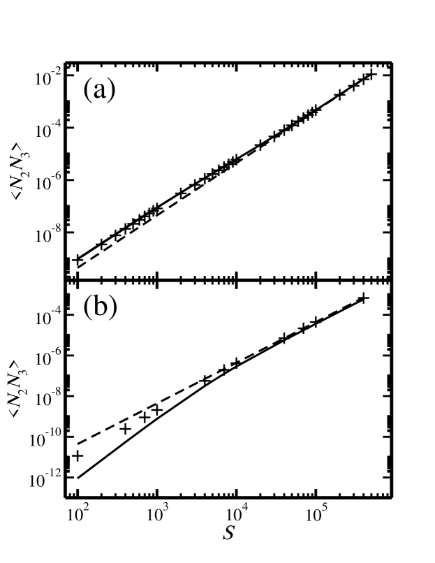
Figure 5: (a) The second moment $\langle N_{2}N_{3}\rangle$ of $P(n_{1},n_{2},n_{3})$ vs. $S$, obtained from the multiplane method (+) for the network shown in Fig. 1(a). This moment is not related to any reaction rate, thus the multiplane method is not designed to approximate it well. Still, it turns out that the results are in good agreement with the master equation (solid line). The rate equation results for the corresponding term, $\langle N_{2}\rangle\langle N_{3}\rangle$, are also shown (dashed line); (b) The moment, $\langle N_{2}N_{3}\rangle$, vs. $S$ for the network shown in Fig. 1(b). The multiplane results (+) deviate from those of the master equation (solid line) in the limit of small grains. For large grains the multiplane results coincide with the master equation and with the corresponding term, $\langle N_{2}\rangle\langle N_{3}\rangle$, of the rate equations (dashed line).

While the second moments which involve pairs of species in the same clique account for their reaction rate, such moments for species from different cliques have no direct physical interpretation. Still, they can be used as an additional test for the accuracy of $P_{\rm MP}(n_{1},n_{2},n_{3})$. Clearly, one may not expect the multiplane method to provide accurate results for such moments because the corresponding correlations are neglected. In Fig. 5(a) we show the moment $\langle N_{2}N_{3}\rangle$ vs. grain size as obtained from the multiplane equations for the reaction network of Fig. 1(a) (+). Surprisingly, the results are in agreement with those of the master equation (solid line). The corresponding rate equation results for $\langle N_{2}\rangle\langle N_{3}\rangle$, are also shown (dashed line). In Fig 5(b) we show the moment $\langle N_{2}N_{3}\rangle$ vs. grain size, as obtained from the multiplane equations (+) for the network of in Fig. 1(b). In this network, the species $X_{3}$ is the result of the reaction between $X_{1}$ and $X_{2}$, enhancing the correlations between them. Indeed, the results of the multiplane method deviate from the master equation results (solid line) in the regime of small grains. However, for large grains the results of the multiplane method and the master equation coincide and agree with those of the rate equations (dashed line). In general, we find that for higher moments of the form $\langle N_{1}^{a}N_{2}^{b}N_{2}^{c}\rangle$, $a,b,c=1,2,\dots$, that involve species from more than one clique, the multiplane method is not reliable in the limit of small grains. For large grains the multiplane and master equation results coincide.

V Analysis of the Method

V.1 The Limit of Small Grains

Consider the probability distribution $P(n_{1},n_{2},n_{3})$ in the limit of small grains, where the average population sizes satisfy $\langle N_{i}\rangle\ll 1$ for $i=1,2,3$. In this limit, $\langle N_{i}\rangle$ can be expressed by $\langle N_{i}\rangle\simeq\rho_{i}\epsilon$, where $\rho_{i}\leq 1$ is a constant that depends on the parameters and $\epsilon\ll 1$ is proportional to the grain size, $S$. In this case, $P(0,0,0)$ is the highest probability while $P(1,0,0)$, $P(0,1,0)$ and $P(0,0,1)$ are of order $\epsilon$. The probability $P(0,1,1)$ of having a pair of $X_{2}$ and $X_{3}$ atoms reside simultaneously on the grain is of order $\epsilon^{2}$. The probabilities $P(1,1,0)$ and $P(1,0,1)$, of having pairs of atoms of species that react with each other reside simultaneously on the grain, are reduced due to the reactions and go like $\epsilon^{3}$. Under these circumstances, the average population sizes satisfy

$$\langle N_{1}\rangle \simeq P(1,0,0)+\mathcal{O}(\epsilon^{2})$$

$$\langle N_{2}\rangle \simeq P(0,1,0)+\mathcal{O}(\epsilon^{2})$$

$$\langle N_{3}\rangle \simeq P(0,0,1)+\mathcal{O}(\epsilon^{2}),$$ (13)

while the second moments that determine the reaction rates satisfy

$$\langle N_{1}N_{2}\rangle \simeq P(1,1,0)+\mathcal{O}(\epsilon^{4})$$

$$\langle N_{1}N_{3}\rangle \simeq P(1,0,1)+\mathcal{O}(\epsilon^{4}).$$ (14)

Using these relations, one can show that in the limit of small grains, to first order in $\epsilon$, the population sizes of $X_{2}$ and $X_{3}$ are statistically independent, namely

$$P(n_{2},n_{3})\simeq P(n_{2})P(n_{3})+\mathcal{O}(\epsilon^{3}).$$ (15)

To show this relation, one needs to examine three states of $(N_{2},N_{3})$, namely $(n_{2},n_{3})=(0,0)$, $(0,1)$ and $(1,0)$. In all other cases, $P(n_{2},n_{3})$ goes like the quadratic or a higher degree of $\epsilon$. As an example, we show that $P(N_{2}=0,N_{3}=0)\simeq P(N_{2}=0)P(N_{3}=0)$, to leading order in $\epsilon$. To this end, we evaluate the left hand side

$$P(N_{2}=0,N_{3}=0)=P(0,0,0)+P(1,0,0)+\mathcal{O}(\epsilon^{2}),$$ (16)

and the right hand side

$$P(N_{2}=0)P(N_{3}=0) = \left[1-P(N_{2}=1)+\mathcal{O}(\epsilon^{2})\right]\left[1-P(N_{3}=1)+\mathcal{O}(\epsilon^{2})\right]$$ (17)

$$= P(0,0,0)+P(1,0,0)+\mathcal{O}(\epsilon^{2}).$$

Clearly, the relation (15) is satisfied. This result justifies the applicability of Eq. (6) in the limit of small grains.

The calculation of mixed second moments for pairs of species that belong to different cliques, such as $\langle N_{2}N_{3}\rangle$ involves probabilities such as $P(N_{2}=1,N_{3}=1)$ for states in which species that do not react with each other reside simultaneously on the grain. It can be shown that these probabilities do not satisfy the relation of Eq. (15). This result is consistent with the fact that the multiplane method does not provide accurate results for this moment, as already observed in Fig. 5(b).

These results further support the conclusion that the multiplane method is suitable for the calculation of moments confined to a single clique and is unsuitable for moments that combine different cliques. To test this conclusion in detail we define the ratio

$$\eta(n_{1},n_{2},n_{3})={P_{\rm MP}(n_{1},n_{2},n_{3})\over P(n_{1},n_{2},n_{3})},$$ (18)

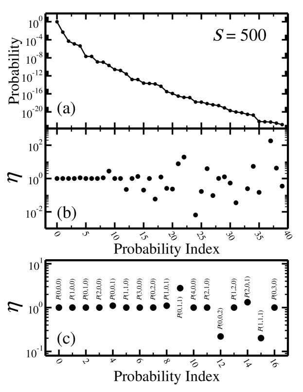
Figure 6: (a) The probabilities $P(n_{1},n_{2},n_{3})$, obtained from the master equation, arranged in descending order from the largest (left) to the smallest (right) for a small grain with $S=500$ adsorption sites. Here we show the forty largest probabilities; (b) The ratio parameter, $\eta$, defined in Eq. (18), between the probabilities obtained from the multiplane equations and the corresponding probabilities obtained from the master equation. The ratio is unity for the first few probabilities and then it fluctuates for the the rest; (c) An enlargement of the first seventeen probabilities displayed in (b). Standing out are $P(0,1,1)$ and $P(1,1,1)$, for which the multiplane equations and the master equation differ. These probabilities have no significant effect on the production rates and population sizes, but are expressed when computing other moments.

which is equal to 1 where the multiplane method is accurate and deviates from 1 elsewhere. In Fig. 6(a) we display the forty highest probabilities, $P(n_{1},n_{2},n_{3})$, obtained from the master equation for the network of Fig. 1(b) in descending order. The results are for a small grain of $S=500$ adsorption sites, for which the population sizes of adsorbed species are exceedingly small. The probabilities drop off very rapidly, implying that the first and second moments are indeed dominated by the few highest probabilities. In Fig. 6(b) we show the parameter $\eta$, for the same set of probabilities. It is confirmed that the multiplane method is valid only for the largest probabilities. Beyond the first few entries, $\eta$ begins to fluctuate. In Fig. 6(c) we show an enlarged plot of $\eta$, including the first 17 probabilities. In this graph the probabilities are labeled. It is found that for those probabilities associated with states in which only species from a single clique reside simultaneously on a grain, the multiplane method is in excellent agreement with the master equation. For states in which species from different cliques reside simultaneously on the grain, significant deviations are obtained. The first significant deviation between the multiplane method and the master equation is found for the probability $P(0,1,1)$, in agreement with the previous analysis.

The analysis above shows that the multiplane method is valid in the limit of small grains. In this limit, the probability distribution is dominated be a few high probabilities associated with small population sizes of the reactive species. These dominant probabilities satisfy the approximation of Eq. (6). Therefore, the population sizes and reaction rates obtained from the multiplane method and the master equation are in excellent agreement.

V.2 The Limit of Large Grains

The applicability of the multiplane method in the limit of large grains is not surprising because in this limit even the rate equations provide accurate results. As shown above, the rate equations can be derrived from the multiplane equations by removing the conditions from the conditional averages. The accuracy of the rate equations shows that in the limit of large grains the correlations are negligible and the probability distribution $P(n_{1},n_{2},n_{3})$ can be factorized into a product of probabilities of single-species. Therefore, the multiplane method provides accurate results for any desired moments of the probability distribution.

VI The Multiplane Equations for Complex Networks

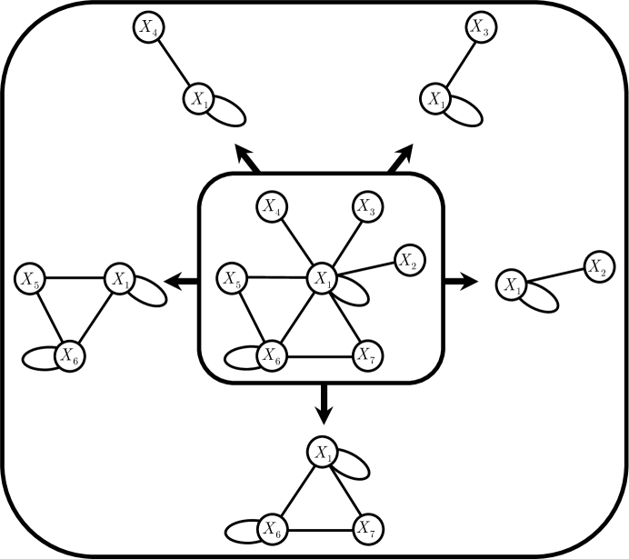
Figure 7: A graph that represents a complex reaction network which consists of seven reactive species. In the multiplane method, this network is broken into five cliques, and a lower dimensional master equation is constructed for the marginal probability distribution associated with each clique. In interstellar chemistry, this is the network leading to the formation of methanol on dust-grain surfaces.

For sparse reaction networks with fluctuations, the multiplane method was found to provide a dramatic reduction in the number of equations compared to the master equation. The method provides accurate results for the populations of reactive species and for the reaction rates. The method was presented for simple networks which include only three species. However, the generalization to more complex networks is straightforward. Consider the network shown in Fig. 7. The probability distribution of the population sizes of the reactive species in this network is $P(n_{1},\dots,n_{7})$. To derive the multiplane equations one first needs to split the network into maximal cliques, or maximal fully-connected subgraphs. For the network of Fig. 7 these cliques are: $C_{1}:\{X_{1},X_{2}\}$, $C_{2}:\{X_{1},X_{3}\}$, $C_{3}:\{X_{1},X_{4}\}$, $C_{4}:\{X_{1},X_{5},X_{6}\}$ and $C_{5}:\{X_{1},X_{6},X_{7}\}$. The next step is to write down the master equation for the marginal probability distribution associated with each clique. This can be done using either the top-down approach, which is straightforward but tedious, or the bottom-up approach.

In the top-down approach, the master equation for the marginal probability distribution associated with a given clique is obtained by tracing over all the species that do not belong to this clique. This procedure is repeated for each one of the maximal cliques.

In the bottom-up approach, the master equation for the internal reactions in each clique is constructed first. Then, the coupling terms between cliques, which include the conditional averages are added one by one. These terms account for reactions between species, such as $X_{j}$, which belong to the clique and species, such as $X_{k}$, which do not belong to the clique. In the master equation, the reaction between $X_{j}$ and $X_{k}$ is described by terms of the form $n_{j}n_{k}P(\dots,n_{j},n_{k},\dots)$. In the multiplane equation for the given clique, $n_{k}$ is replaced by $\langle N_{k}\rangle_{n_{j}}$ and $P(\dots,n_{j},n_{k},\dots)$ is replaced by the marginal probability distribution for the clique. For example, the resulting equation for the clique $C_{1}$ is

$$\dot{P}(n_{1},n_{2}) = F_{1}[P(n_{1}-1,n_{2})-P(n_{1},n_{2})]$$

$$+ F_{2}[P(n_{1},n_{2}-1)-P(n_{1},n_{2})]$$

$$+ W_{1}[(n_{1}+1)P(n_{1}+1,n_{2})-n_{1}P(n_{1},n_{2})]$$

$$+ W_{2}[(n_{2}+1)P(n_{1},n_{2}+1)-n_{2}P(n_{1},n_{2})]$$

$$+ (A_{1}+A_{2})[(n_{1}+1)(n_{2}+1)P(n_{1}+1,n_{2}+1)-n_{1}n_{2}P(n_{1},n_{2})]$$

$$+ A_{1}[(n_{1}+2)(n_{1}+1)P(n_{1}+2,n_{2})-n_{1}(n_{1}-1)P(n_{1},n_{2})]$$

$$+ \sum_{i=3}^{7}{(A_{1}+A_{i})[(n_{1}+1)\langle N_{i}\rangle_{n_{1}+1}P(n_{1}+1,n_{2})-n_{1}\langle N_{i}\rangle_{n_{1}}P(n_{1},n_{2})]},$$

where Eq. (6) is used in order to justify the replacement of $\langle N_{i}\rangle_{n_{1},n_{2}}$ by $\langle n_{i}\rangle_{n_{1}}$. We find it instructive to carry out the procedure for the clique $C_{5}$ as well. In this clique, the species $X_{1}$ and $X_{6}$ are both correlated with $X_{5}$. When tracing over $X_{5}$ one must maintain both correlations, giving rise to the conditional average $\langle N_{5}\rangle_{n_{1},n_{6}}$. The resulting equation takes the form:

$$\dot{P}(n_{1},n_{6},n_{7}) = \sum_{i=1,6,7}F_{i}[P(\dots,n_{i}-1,\dots)-P(n_{1},n_{6},n_{7})]$$

$$+ \sum_{i=1,6,7}W_{i}[(n_{i}+1)P(\dots,n_{i}+1,\dots)-n_{i}P(n_{1},n_{6},n_{7})]$$

$$+ (A_{1}+A_{6})[(n_{1}+1)(n_{6}+1)P(n_{1}+1,n_{6}+1,n_{7})-n_{1}n_{6}P(n_{1},n_{6},n_{7})]$$

$$+ (A_{1}+A_{7})[(n_{1}+1)(n_{7}+1)P(n_{1}+1,n_{6},n_{7}+1)-n_{1}n_{7}P(n_{1},n_{6},n_{7})]$$

$$+ (A_{6}+A_{7})[(n_{6}+1)(n_{7}+1)P(n_{1},n_{6}+1,n_{7}+1)-n_{6}n_{7}P(n_{1},n_{6},n_{7})]$$

$$+ \sum_{i=1,6}A_{i}[(n_{i}+2)(n_{i}+1)P(\dots,n_{i}+2,\dots)-n_{i}(n_{i}-1)P(n_{1},n_{6},n_{7})]$$

$$+ \sum_{i=2}^{4}{(A_{1}+A_{i})[(n_{1}+1)\langle N_{i}\rangle_{n_{1}+1}P(n_{1}+1,n_{6},n_{7})-n_{1}\langle N_{i}\rangle_{n_{1}}P(n_{1},n_{6},n_{7})]}$$

$$+ (A_{1}+A_{5})[(n_{1}+1)\langle N_{5}\rangle_{n_{1}+1,n_{6}}P(n_{1}+1,n_{6},n_{7})-n_{1}\langle N_{5}\rangle_{n_{1},n_{6}}P(n_{1},n_{6},n_{7})]$$

$$+ (A_{5}+A_{6})[(n_{6}+1)\langle N_{5}\rangle_{n_{1},n_{6}+1}P(n_{1},n_{6}+1,n_{7})-n_{6}\langle N_{5}\rangle_{n_{1},n_{6}}P(n_{1},n_{6},n_{7})].$$

This network has been simulated using both the multiplane method and the complete master equation. The results were found to be in excellent agreement Lipshtat2004 .

VII Applications to Physical and Biological Systems

Stochastic simulations are of great importance in a wide range of physical systems. Below we present two examples of current research areas in which the multiplane method is expected to be useful.

VII.1 Chemical Networks on Interstellar Grains

The chemistry of interstellar clouds includes gas-phase reactions as well as grain-surface reactions Hartquist1995 ; Tielens2005 . Due to the microscopic size of the grains, and the low flux, the population sizes of reactive species on the grains may be small and exhibit strong fluctuations. Under these conditions rate equations are not suitable for the simulation of grain-surface chemistry Tielens1982 ; Charnley1997 ; Caselli1998 ; Shalabiea1998 . To account correctly for the reaction rates, stochastic methods such as direct integration of the master equation Biham2001 ; Green2001 ; Biham2002 or Monte Carlo simulations Tielens1982 ; Charnley1997 ; Charnley2001 are required. The master equation is more suitable for grain chemistry because it consists of differential equations, which can be easily coupled to the rate equations of gas phase chemistry. Furthermore, the master equation provides the probability distribution from which the reaction rates can be evaluated directly, unlike Monte Carlo methods that require to accumulate large sets of data and to perform ensemble or temporal averages. For simple networks the master equation is efficient and provides accurate results. However, for complex networks, the master equation becomes infeasible. In this case, the multiplane method provides efficient stochastic simulations.

Consider the network of Fig. 7. Using the following substitutions $X_{1}\rightarrow\rm{H};X_{2}\rightarrow\rm{OH};X_{3}\rightarrow\rm{H}_{3}\rm{CO};X_{4}\rightarrow\rm{H}_{2}\rm{CO};X_{5}\rightarrow\rm{HCO};X_{6}\rightarrow\rm{O};X_{7}\rightarrow\rm{CO}$, this network coincides with the reaction network that leads to methanol production on grains in molecular clouds Tielens1982 ; Charnley1997 ; Stantcheva2002 ; Stantcheva2003 ; Lipshtat2004 . Current experimental effort is aimed at the evaluation of the relevant rate constants for the surface diffusion, reaction and desorption of the species involved in this network Perets2005 ; Hidaka2007 . These experiments include infra-red spectroscopy as well as temperature-programmed desorption runs using a mass spectrometer to detect the desorbed molecules. The resulting parameters, inserted into the multiplane equations, will enable to evaluate the reaction rates in interstellar environments and to compare the results with observations. The multiplane method for this network provides a reduction in the number of equations from about one million, using the master equation, to about one thousand equations. For more complex networks the master equation becomes infeasible while the multiplane method remains efficient.

VII.2 Genetic Networks in Cells

Another important field in which the multiplane method is expected to be useful is the study of genetic regulatory networks in cells. These networks describe the transcription of mRNAs from genes and their translation into proteins. The regulation is performed at the transcriptional level (by transcription factors that bind to the promoter site of the regulated gene), at the post-trancriptional level (e.g., by small non-coding RNAs) and at the post-translational level (e.g., by protein-protein interactions). Analysis of these networks revealed modular structure. In particular, modules or motifs which perform specific functions and repeatedly appear in different parts of the network were identified Milo2002 ; Milo2004 ; Yeger-Lotem2004 . Common examples of such motifs are the autorepressor Rosenfeld2002 and different versions of the feed forward loop Mangan2003 . Other modules such as the genetic switch Ptashne1992 and the mixed-feedback loop Francois2005 also appear, but are not as common.

Genetic networks often exhibit strong fluctuations due to the fact that some of the transcription factors appear in low copy numbers. Moreover, the transcriptional regulation is typically performed by a small number of transcription factors which bind and unbind to the promoter site at a fast rate. This gives rise to strong fluctuations in the transcription rate of the regulated gene. Some modules, such as the autorepressor, the genetic switch and the mixed-feedback loop include positive or negative feedback mechanisms, which tend to enhance the role of fluctuations. In particular, the dynamics of the genetic switch system was studied extensively using both deterministic and stochastic methods Gardner2000 ; Kepler2001 ; Cherry2000 ; Warren2004 ; Warren2005 ; Walczak2005 ; Lipshtat2006 ; Loinger2007 . It was found that fluctuations play a crucial role in this system. While the analysis of small modules such as the genetic switch can be done using the master equation, it quickly becomes infeasible when larger networks are considered. The implementation of the multiplane method in this context is expected to provide a broader perspective on the role of fluctuations in genetic networks. Recently, such fluctuations at the level of single cells were measured experimentally using the green fluorescent protein Elowitz2002 . Such measurements are also expected to provide the effective rate constants of the relevant processes in the cell.

VIII Summary and Discussion

We have shown that the multiplane method provides efficient simulations of complex reaction networks with fluctuations, for which the rate equations fail and the master equation is infeasible. The multiplane equations are obtained by breaking the network into maximal cliques and writing down the set of master equations for the marginal probability distributions of these cliques, with a suitable coupling between them. For typical sparse networks, the method provides a dramatic reduction in the number of equations. We found that the multiplane results for the first and second moments, which account for population sizes and reaction rates, respectively, are in excellent agreement with those of the complete master equation. It also accounts correctly for higher moments which involve species from the same clique. However, the method does not account correctly for second and higher moments which include species from different cliques.

The numerical results are complemented by an asymptotic analysis of the small and large grain limits. A more rigorous analysis shows that the multiplane method is asymptotically exact in both limits Barzel2007 . It is performed in a more general setting, in which the maximal cliques may be broken into smaller cliques. In particular, one may break the entire network into cliques of two species each. It is shown that even in this case, in the limits of small and large grains, the method still provides exact results for all the first moments and for those second moments that involve species in the same clique.

A related approach, based on moment equations, also provides efficient stochastic simulations of reaction networks Barzel2007a . In this approach, one constructs differential equations for the first and second moments of the probability distribution. The number of equations is further reduced to one equation for each reactive species (node) and one equation for each reaction (edge). Thus, for typical sparse networks the complexity of the stochastic simulation becomes comparable to that of the rate equations. In applications such as interstellar chemistry, in which the main objective is to calculate the reaction rates, the moment equations are advantageous. However, in systems such as genetic networks, in which the probability distribution itself is of interest, the multiplane method is required.

References

- (1) N.G. van Kampen, Stochastic Processes in Physics and Chemistry (North-Holland, Amsterdam, 1981).
- (2) D.A. McQuarrie, J. Appl. Prob. 4, 413 (1967).
- (3) O. Biham, I. Furman, V. Pirronello and G. Vidali, Astrophys. J. 553, 595 (2001).
- (4) N.J.B. Green, T. Toniazzo, M.J. Pilling, D.P. Ruffle, N. Bell and T.W. Hartquist, Astron. Astrophys. 375, 1111 (2001).
- (5) O. Biham and A. Lipshtat, Phys. Rev. E 66, 056103 (2002).
- (6) T. Stantcheva, V.I. Shematovich and E. Herbst, Astron. Astrophys. 391, 1069 (2002).
- (7) T. Stantcheva and E. Herbst, Mon. Not. R. Astron. Soc. 340, 983 (2003).
- (8) A. Lipshtat, O. Biham, Phys. Rev. Lett. 93, 170601 (2004).
- (9) A.G.G.M. Tielens and W. Hagen, Astron. Astrophys. 114, 245 (1982).
- (10) S.B. Charnley, A.G.G.M. Tielens and S.D. Rodgers, Astrophys. J. 482, L203 (1997).
- (11) P. Caselli, T.I. Hasegawa and E. Herbst, Astrophys. J. 495, 309 (1998).
- (12) O.M. Shalabiea, P. Caselli and E. Herbst, Astrophys. J. 502, 652 (1998).
- (13) J. Paulsson and M. Ehrenberg, Phys. Rev. Lett. 84, 5447 (2000).
- (14) J. Paulsson, O.G. Berg and M. Ehrenberg, Proc. Natl. Acad. Sci. US 97, 7148 (2000).
- (15) J. Paulsson, Nature 427, 415 (2004).
- (16) D.T. Gillespie, J. Phys. Chem. 81, 2340 (1977).
- (17) H.H. McAdams and A. Arkin, 94, 814 (1997).
- (18) H.H. McAdams and A. Arkin, 15, 65 (1999).
- (19) A. Lipshtat, O. Biham, Phys. Rev. E 66, 056103 (2002).
- (20) I. Lohmar and J. Krug, Mon. Not. R. Astron. Soc. 370, 1025 (2006).
- (21) T. Stantcheva, P. Caselli and E. Herbst, Astron. Astrophys. 375, 673 (2001).
- (22) T.W. Hartquist and D.A. Williams, The chemically controlled cosmos (Cambridge University Press, Cambridge, UK, 1995).
- (23) A.G.G.M. Tielens, The Physics and Chemistry of the Interstellar Medium (Cambridge University Press, Cambridge, 2005).
- (24) S.B. Charnley, Astrophys. J. 562, L99 (2001).
- (25) H.B. Perets, O. Biham, V. Pirronello, J.E. Roser, S. Swords, G. Manico and G. Vidali, Astrophys. J. 627, 850 (2005).
- (26) H. Hidaka, A. Kouchi and N. Watanabe, J. Chem. Phys. 126, 204707 (2007)
- (27) R. Milo, S. Shen-Orr, S. Itzkovitz, N. Kashtan, D. Chklovskii and U. Alon, Science 298, 824 (2002).
- (28) R. Milo, S. Itzkovitz, N. Kashtan, R. Levitt, S. Shen-Orr, I. Ayzenshtat, M. Sheffer and U. Alon, Science 303, 1538 (2004).
- (29) E. Yeger-Lotem, S. Sattath, N. Kashtan, S. Itzkovitz,R. Milo, R.Y. Pinter, U. Alon and H. Margalit, Proc. Natl. Acad. Sci. US 101, 5934 (2004).
- (30) N. Rosenfeld, M.B. Elowitz and U. Alon, J. Mol. Biol. 323, 785 (2002).
- (31) S. Mangan and U. Alon, Proc. Natl. Acad. Sci. US 100, 11980 (2003).
- (32) M. Ptashne, A Genetic Switch: Phage and Higher Organisms, 2nd edition. (Cell Press and Blackwell Scientific Publications, Cambridge, MA, 1992).
- (33) P. Francois and V. Hakim, Phys. Rev. E 72, 031908 (2005).
- (34) T.S. Gardner, C.R. Cantor and J.J. Collins, Nature 403, 339 (2000).
- (35) T.B. Kepler and T.C. Elston, Biophysical Journal 81, 3116 (2001).
- (36) J.L. Cherry and F.R. Adler, J. Theor. Biol. 203, 117 (2000).
- (37) P.B. Warren and P.R. ten Wolde, Phys. Rev. Lett. 92, 128101 (2004).
- (38) P.B. Warren and P.R. ten Wolde, J. Phys. Chem. B 109, 6812 (2005).
- (39) A. M. Walczak, M. Sasai, and P. Wolynes, Biophysical Journal 88, 828 (2005).
- (40) A. Lipshtat, A. Loinger, N.Q. Balaban and O. Biham, Phys. Rev. Lett. 96, 188101 (2006).
- (41) A. Loinger, A. Lipshtat, N. Q. Balaban and O. Biham, Phys. Rev. E 75, 021904 (2007).
- (42) M.B. Elowitz, A.J. Levine, E.D. Siggia and P.S. Swain, Science 297, 1183 (2002).
- (43) B. Barzel, O. Biham and R. Kupferman, to be submitted to SIAM Multiscale Modeling and Simulation (2007).
- (44) B. Barzel and O. Biham, Astrophys. J. 658, L37 (2007).