A Method for Weak Lensing Flexion Analysis by the HOLICs Moment Approach

Abstract

We have developed a method for measuring higher-order weak lensing distortions of faint background galaxies, namely the weak gravitational flexion, by fully extending the Kaiser, Squires & Broadhurst method to include higher-order lensing image characteristics (HOLICs) introduced by Okura, Umetsu, & Futamase. We take into account explicitly the weight function in calculations of noisy shape moments and the effect of higher-order PSF anisotropy, as well as isotropic PSF smearing. Our HOLICs formalism allows accurate measurements of flexion from practical observational data in the presence of non-circular, anisotropic PSF. We test our method using mock observations of simulated galaxy images and actual, ground-based Subaru observations of the massive galaxy cluster A1689 ($z=0.183$). From the high-precision measurements of spin-1 first flexion, we obtain a high-resolution mass map in the central region of A1689. The reconstructed mass map shows a bimodal feature in the central $4^{\prime}\times 4^{\prime}$ region of the cluster. The major, pronounced peak is associated with the brightest cluster galaxy and central cluster members, while the secondary mass peak is associated with a local concentration of bright galaxies. The refined, high-resolution mass map of A1689 demonstrates the power of the generalized weak lensing analysis techniques for quantitative and accurate measurements of the weak gravitational lensing signal.

1 Introduction

Propagation of light rays from a distant source to the observer is governed by the gravitational field of intervening mass fluctuations as well as by the global geometry of the universe. The images of background sources hence carry the imprint of the gravitational potential of intervening cosmic structures, and their statistical properties can be used to test the background cosmological models.

Weak gravitational lensing is responsible for the weak shape-distortion and magnification of the images of background sources due to the gravitational field of intervening matter (e.g., Bartelmann & Schneider 2001; Umetsu, Futamase, & Tada 1999). To the first order, weak lensing gives rise to a few – $10\%$ levels of elliptical distortions in images of background sources, responsible for the second-order derivatives of the gravitational lensing potential. Thus, the weak lensing signal, measured from tiny but coherent quadrupole distortions in galaxy shapes, can provide a direct measure of the projected mass distribution of cosmic structures. However, practical weak lensing observations subject to the effects of atmospheric seeing, isotropic/anisotropic PSF, and (residual) camera distortion across the field of view, which must be examined from the stellar shape measurements and corrected for in the weak lensing analysis. Practical methods for PSF corrections and shear measurements/calibrations have been studied and developed by many authors, such as pioneering work of Kaiser, Squires, & Broadhurst (1995, hereafter KSB), the Shapelets technique which describes PSF and object images in terms of Gaussian-Hermite expansions (Refregier 2003), and recent systematic, collaborative efforts by The Shear TEsting Programme (Heymans et al. 2006; Massey et al. 2007).

Thanks to these successful developments in weak lensing techniques as well as in instrument technology, the quadrupole weak lensing has become one of the most important tools in observational cosmology to map the mass distribution in individual clusters of galaxies (e.g., Kaiser & Squires 1993; Broadhurst et al. 2005a; Okabe & Umetsu 2007; Umetsu & Broadhurst 2007), measure ensemble-averaged mass profiles of galaxy-group sized halos from the galaxy-galaxy lensing signal (e.g., Hoekstra et al. 2001; Hoekstra et al. 2004; Parker et al. 2005; Mandelbaum et al. 2006), study the statistical properties of the large scale structure of the universe from the cosmic shear statistics (e.g., Bacon et al. 2000; van Waerbeke et al. 2001; Hamana et al. 2003), and search for galaxy clusters by their mass properties (e.g., Schneider 1996; Erben et al. 2000; Umetsu & Futamase 2000; Wittman et al. 2001).

In recent years, there have been theoretical efforts to include the next higher order distortion effects as well as the usual quadrupole distortion effect in the weak lensing analysis (Goldberg & Natarajan 2002; Goldberg & Bacon 2005; Bacon et al. 2006; Irwin & Shmakova 2006; Goldberg & Leonard 2007; Okura, Umetsu, & Futamase 2007). We have proposed in Okura, Umetsu, & Futamase (2007, hereafter OUF) to use certain convenient combinations of octopole/higher multipole moments of background images which we call the Higher Order Lensing Image’s Characteristics (HOLICs), and have shown that HOLICs serve as a direct measure for the next higher-order weak lensing effect, or the gravitational flexion (Goldberg & Bacon 2005) and that the use of HOLICs in addition to the quadrupole shape distortions can improve the accuracy and resolution of weak lensing mass reconstructions based on simulated observations.

Recently, Goldberg & Leonard (2007) extended the HOLICs approach for flexion measurements to include observational effects, namely the Gaussian weighting in shape-moment calculations (see the appendix therein) and the isotropic PSF effect, under the assumption that PSF is nearly circular, and tested their extended HOLICs approach with simulated and HST/ACS observations. Leonard et al. (2007) have applied the extended HOLICs method to reconstruct the projected mass distribution in the central region of the massive galaxy cluster A1689 at $z=0.183$, and revealed substructures associated with small clumps of galaxies. Further Leonard et al. (2007) found that in dense systems such as galaxy clusters the HOLICs technique is robust and less sensitive than the Shapelet technique to contamination by light from the extended wings of lens/foreground galaxies.

In the present paper we develop a method for measuring flexion by the HOLICs approach by fully extending the KSB formalism; We take into account explicitly the effects of Gaussian weighting in calculation of noisy shape moments and higher-order PSF anisotropy as well as isotropic PSF smearing. We then apply our method to actual, ground-based Subaru observations of A1689, and perform a mass reconstruction in the central region of A1689.

The paper is organized as follows. We first summarize in §2 the basis of weak gravitational lensing and the flexion formalism. In §3, we derive the relationship between HOLICs and flexion by incorporating Gaussian smoothing in shape measurements in the presence of isotropic and anisotropic PSF. The practical method to correct the isotropic/anisotropic PSF effects will be presented in §4. In Section 5 we use simulations to test our flexion analysis method based on the HOLICs moment approach. We then perform a weak lensing flexion analysis of A1689 by our fully-extended HOLICs approach, and perform a mass reconstruction of A1689 from the HOLICs estimates of flexion. Finally summary and discussions are given in §6. We refer interested readers to a complete appendix for details of the derivation of flexion-observable relationships in practical observations.

2 Basis of Weak Lensing and Flexion

In this section, we summarize general aspects of weak gravitational lensing and flexion formalism, following the complex derivative notation developed by Bacon et al. (2006). A general review of quadrupole weak lensing can be found in Bartelmann & Schneider (2001).

2.1 Spin Properties

We define the spin for weak-lensing quantities in the following way: A quantity is said to have spin $N$ if it has the same value after rotation by $2\pi/N$. The product of spin-$A$ and spin-$B$ quantities has spin $(A+B)$, and the product of spin-$A$ and spin-$B^{*}$ quantities has spin $(A-B)$. Then, as we shall see in the next subsection, the lensing convergence $\kappa$ is a spin-0 (scalar) quantity. The complex shear $\gamma$ and the reduced shear $g=\gamma/(1-\kappa)$ are spin-2 quantities. The first and second flexion fields, $F$ and $G$, are a spin-1 and a spin-3 quantity, respectively.

2.2 Weak Lensing and Flexion Formalism

The gravitational deflection of light rays can be described by the lens equation,

$$\mbox{\boldmath$\beta$}=\mbox{\boldmath$\theta$}-\mbox{\boldmath$\nabla$}\psi(\mbox{\boldmath$\theta$}),$$ (1)

where $\psi(\mbox{\boldmath$\theta$})$ is the effective lensing potential, which is defined by the two-dimensional Poisson equation as $\nabla^{2}\psi(\mbox{\boldmath$\theta$})=2\kappa(\mbox{\boldmath$\theta$})$, with the lensing convergence. Here the convergence $\kappa=\int\!d\Sigma_{m}\Sigma_{\rm crit}^{-1}$ is the dimensionless surface mass density projected on the sky, normalized with respect to the critical surface mass density of gravitational lensing,

$$\Sigma_{\rm crit}=\frac{c^{2}}{4\pi G}\frac{D_{s}}{D_{d}D_{ds}},$$ (2)

where $D_{d}$, $D_{s}$, and $D_{ds}$ are the angular diameter distances from the observer to the deflector, from the observer to the source, and from the deflector to the source, respectively. By introducing the complex gradient operator, $\partial=\partial_{1}+i\partial_{2}$ that transforms as a vector, $\partial^{\prime}=\partial e^{i\phi}$, with $\phi$ being the angle of rotation, the lensing convergence $\kappa$ is expressed as

$$\kappa=\frac{1}{2}\partial\partial^{*}\psi,$$ (3)

where ^∗ denotes the complex conjugate. Similarly, the complex gravitational shear of spin-2 is defined as

$$\gamma\equiv\gamma_{1}+i\gamma_{2}=\frac{1}{2}\partial\partial\psi.$$ (4)

The third-order derivatives of $\psi(\mbox{\boldmath$\theta$})$ can be combined to from a pair of the complex flexion fields as (Bacon et al. 2006):

$${\cal F} \equiv {\cal F}_{1}+i{\cal F}_{2}=\frac{1}{2}\partial\partial\partial^{*}\psi,$$ (5)

$${\cal G} \equiv {\cal G}_{1}+i{\cal G}_{2}=\frac{1}{2}\partial\partial\partial\psi.$$ (6)

If the angular size of an image is small compared to the scale over which the lens potential $\psi$ varies, then we can locally expand the lens equation (1) to have:

$$d\beta_{i}={\cal A}_{ij}d\theta_{j}+\frac{1}{2}{\cal D}_{ijk}d\theta_{j}d\theta_{k}$$ (7)

to the second order, where ${\cal A}_{ij}$ is the Jacobian matrix of the lens equation and ${\cal D}_{ijk}={\cal A}_{ij,k}=-\psi_{,ijk}$ is the third-order lensing tensor,

$${\cal A}_{ij} = \left(\begin{array}[]{cc}1-{\kappa}-{\gamma}_{1}&-{\gamma}_{2}\\ -{\gamma}_{2}&1-{\kappa}+{\gamma}_{1}\end{array}\right),$$ (10)

$${\cal D}_{ijk} = {\cal F}_{ijk}+{\cal G}_{ijk}.$$ (11)

The third-order tensor ${\cal D}_{ijk}$ can be expressed with the sum of the two terms, ${\cal D}_{ijk}={\cal F}_{ijk}+{\cal G}_{ijk}$, with the spin-1 part ${\cal F}_{ijk}$ and the spin-3 part ${\cal G}_{ijk}$, composed of the real/imaginary part of the flexion fields:

$${\cal F}_{ij1}=-\frac{1}{2}\left(\begin{array}[]{@{\,}cc@{\,}}3{\cal F}_{1}&{\cal F}_{2}\\ {\cal F}_{2}&{\cal F}_{1}\end{array}\right) \ \ {\cal F}_{ij2}=-\frac{1}{2}\left(\begin{array}[]{@{\,}cc@{\,}}{\cal F}_{2}&{\cal F}_{1}\\ {\cal F}_{1}&3{\cal F}_{2}\end{array}\right),$$ , (16)

$${\cal G}_{ij1}=-\frac{1}{2}\left(\begin{array}[]{@{\,}cc@{\,}}{\cal G}_{1}&{\cal G}_{2}\\ {\cal G}_{2}&-{\cal G}_{1}\end{array}\right) \ \ {\cal G}_{ij2}=-\frac{1}{2}\left(\begin{array}[]{@{\,}cc@{\,}}{\cal G}_{2}&-{\cal G}_{1}\\ -{\cal G}_{1}&-{\cal G}_{2}\end{array}\right).$$ , (21)

Note that flexion has a dimension of inverse length (or inverse angle), meaning that the flexion effect depends on the angular size of the source. The shape quantities affected by the first flexion ${\cal F}$ alone have spin-1 properties, while those affected by the second flexion ${\cal G}$ alone have spin-3 properties. These third-order lensing fields naturally appear in the transformation equations of HOLICs between the lens and source planes.

2.3 Quadrupole Lensing Observable – Complex Ellipticity

In the KSB approach, we use quadrupole moments $Q_{ij}$ of the surface brightness distribution $I(\mbox{\boldmath$\theta$})$ of background images for quantifying the shape of the images:

$$Q_{ij}\equiv\frac{\int\!d^{2}\theta\,q_{I}[I(\mbox{\boldmath$\theta$})]\Delta\theta_{i}\Delta\theta_{j}}{\int d^{2}\theta\,q_{I}[I(\mbox{\boldmath$\theta$})]},$$ (22)

where $q_{I}[I(\mbox{\boldmath$\theta$})]$ denotes the weight function used in noisy shape measurements and $\Delta\theta_{i}=\theta_{i}-\bar{\theta}_{i}$ is the offset vector from the image centroid. The complex ellipticity $\chi$ is then defined as

$$\chi\equiv\frac{Q_{11}-Q_{22}+2iQ_{12}}{Q_{11}+Q_{22}},$$ (23)

The $\chi$ transforms under the lens mapping as

$$\chi^{(s)}=\frac{\chi-2g+g^{2}\chi^{\ast}}{1+|g|^{2}-2{\rm Re}\left[g\chi^{\ast}\right]},$$ (24)

where $g=\gamma/(1-\kappa)$ is the spin-2 reduced shear. In the weak lensing limit ($\kappa,|\gamma|\ll 1$), equation (24) reduces to $\chi^{(s)}\approx\chi-2\gamma$. Assuming the random orientation of the background sources, we average observed ellipticities over a sufficient number of images to obtain

$$\langle\chi\rangle\approx 2g\approx 2\gamma.$$ (25)

2.4 Centroid Shift due to Lensing

In the moment methods such as KSB, we quantify the shape of an image by measuring various moments of $I(\mbox{\boldmath$\theta$})$, in which the moments are calculated with respect to the observable centroid of the image $\bar{\mbox{\boldmath$\theta$}}$, or the center of the light, defined by the first moment of $I(\mbox{\boldmath$\theta$})$. However, in the presence of gravitational lensing, this apparent center can be different from the point $\mbox{\boldmath$\theta$}(\bar{\mbox{\boldmath$\beta$}})$ that is mapped using the lens equation (1) from the center of the unlensed light, $\bar{\mbox{\boldmath$\beta$}}$. We refer to this point as the “true” center of the image. The difference between these two centers, namely, the apparent and the true centers, causes a significant effect in evaluating the first flexion, as pointed out by Goldberg & Bacon (2005). The relationship between the two centers is

$$\theta_{i}(\bar{\mbox{\boldmath$\beta$}})\approx\bar{\theta}_{i}-{\rm tr}Q\left(\frac{3}{2}F_{i}+\frac{5}{4}[F^{*}\chi]_{i}+\frac{1}{4}[G\chi^{*}]_{i}\right)\equiv\bar{\theta}_{i}-\Delta_{L,i},$$ (26)

where ${\rm tr}Q=Q_{11}+Q_{22}$ is the trace of $Q_{ij}$, $F$ and $G$ are the reduce Flexion, defined by $F={\cal F}/(1-\kappa)$ and $G={\cal G}/(1-\kappa)$, respectively, and $\Delta_{L,i}$ is the displacement vector from the true to the apparent center due to gravitational lensing. Therefore, by taking into account the centroid shift in shape measurements, we have the relation between $\Delta\beta_{i}=\beta_{i}-\bar{\beta}_{i}$ and $\Delta\theta_{i}=\theta_{i}-\bar{\theta}_{i}$ as

$$\Delta\beta_{i} \approx {\cal A}_{ij}\Delta\theta_{j}+\frac{1}{2}{\cal D}_{ijk}\Delta\theta_{j}\Delta\theta_{k}+{\rm tr}Q\left(\frac{3}{2}F_{i}+\frac{5}{4}[F^{*}\chi]_{i}+\frac{1}{4}[G\chi^{*}]_{i}\right)$$ (27)

$$= {\cal A}_{ij}\Delta{\theta}_{j}+\frac{1}{2}{\cal D}_{ijk}\Delta\theta_{j}\Delta\theta_{k}+\Delta_{L,i}.$$

A detailed derivation of the above relation is given in Appendix B of OUF.

2.5 Flexion Observable – HOLICs

The flexion fields, ${\cal F}$ and ${\cal G}$, can be measured from proper combinations of higher-order shape moments with the corresponding spin properties and the dimension, as explicitly shown by OUF. Higher-order moments of images are defined as a straightforward extension of the quadrupole moment. The octopole moment $Q_{ijk}$ and the 16pole moment $Q_{ijkl}$ are defined as follows:

$$Q_{ijk} \equiv \frac{\int\!d^{2}\theta\,q_{I}[I(\mbox{\boldmath$\theta$})]\Delta\theta_{i}\Delta\theta_{j}\Delta\theta_{k}}{\int d^{2}\theta\,q_{I}[I(\mbox{\boldmath$\theta$})]}$$ (28)

$$Q_{ijkl} \equiv \frac{\int\!d^{2}\theta\,q_{I}[I(\mbox{\boldmath$\theta$})]\Delta\theta_{i}\Delta\theta_{j}\Delta\theta_{k}\Delta\theta_{l}}{\int d^{2}\theta\,q_{I}[I(\mbox{\boldmath$\theta$})]}.$$ (29)

Then, $\zeta$ and $\delta$ of the spin-1 and spin-3 HOLICs, respectively, are defined by

$$\zeta \equiv \frac{Q_{111}+Q_{122}+i\left(Q_{112}+Q_{222}\right)}{\xi}$$

$$\delta \equiv \frac{Q_{111}-3Q_{122}+i\left(3Q_{112}-Q_{222}\right)}{\xi},$$ (30)

where $\xi$ is the spin-0 normalization factor,

$$\xi=Q_{1111}+2Q_{1122}+Q_{2222}.$$ (31)

Finally, the transformation equations between unlensed and lensed HOLICs are obtained as (see OUF)

$$\zeta^{(s)} = \frac{\zeta-2g\zeta^{*}-g^{*}\delta-\frac{1}{4}(8F^{*}\eta-16\frac{\left({\rm tr}Q\right)^{2}}{\xi}F^{*}\chi+9F-12\frac{\left({\rm tr}Q\right)^{2}}{\xi}F+2G\eta^{*}-2\frac{\left({\rm tr}Q\right)^{2}}{\xi}G\chi^{*}+G^{*}\lambda)}{(1-\kappa)(1-4{\rm Re}\left[g^{*}\eta\right]-5{\rm Re}\left[F\iota_{I}^{*}\right]-{\rm Re}\left[G\iota_{III}^{*}\right])},$$

$$\delta^{(s)} = \frac{\delta-3g\zeta-\frac{1}{4}(10F\eta+7F^{*}\lambda-18\frac{\left({\rm tr}Q\right)^{2}}{\xi}F\chi+3G)}{(1-\kappa)(1-4{\rm Re}\left[g^{*}\eta\right]-5{\rm Re}\left[F\iota_{I}^{*}\right]-{\rm Re}\left[G\iota_{III}^{*}\right])},$$ (32)

where $\eta$ and $\lambda$ are dimensionless spin-2 and spin-4 quantities, respectively, defined with 16-pole moments, and $\iota_{I}$, $\iota_{III}$ and $\iota_{V}$ are spin-1, spin-3, and spin-5 quantities, respectively, defined with $32$-pole moments (see Appendix and OUF). We note that, the above equations (2.5) and (32) are obtained under the sub-critical lensing condition, i.e., ${\rm det}{\cal A}>0$ (see Schneider & Er 2007).

Since the HOLICs $\zeta$ and $\delta$ are non-zero spin quantities with a direction dependence, the expectation value of the intrinsic $\zeta$ and $\delta$ are assumed to vanish. To the first order in flexion, we have the linear relations between the HOLICs and flexion fields as

$$F \approx \left<\frac{\zeta}{\frac{9}{4}-3\frac{\left({\rm tr}Q\right)^{2}}{\xi}}\right>$$ (33)

$$G \approx \frac{4}{3}\left<\delta\right>.$$ (34)

3 HOLICs and Flexion in Practical Applications

For a practical application of the HOLICs approach, we must take into account various observational effects such as noise in the shape measurement due to readout and/or sky background and the dilution of the lensing signal due to the isotropic/anisotropic PSF effects. Thus, one cannot simply use equations (2.5) and (32) to measure the flexion fields. In this section, we introduce the Gaussian weighting in moment calculations, as done in the KSB formalism for quadrupole weak lensing, and derive the relevant transformation equations between unlensed and lensed HOLICs by taking into account explicitly the effect of Gaussian smoothing.

3.1 Redefining HOLICs for Noisy Observations

Now we introduce a weight function $W(|\Delta\theta|^{2}/\sigma^{2})$ having a characteristic width $\sigma$ for practical, noisy moment measurements, redefining the octopole and 16-pole moments of the brightness distribution $I(\mbox{\boldmath$\theta$})$ as

$$Q_{ijk} \equiv \int d^{2}\theta I(\theta)\Delta\theta_{i}\Delta\theta_{j}\Delta\theta_{k}W(|\Delta\theta|^{2}/\sigma^{2}),$$ (35)

$$Q_{ijkl} \equiv \int d^{2}\theta I(\theta)\Delta\theta_{i}\Delta\theta_{j}\Delta\theta_{k}\Delta\theta_{l}W(|\Delta\theta|^{2}/\sigma^{2}),$$ (36)

where $Q$s here are no longer normalized with the corresponding flux of the image (see equation [22]). The redefined shape moments enter equation (2.5). We provide in Appendix detailed definitions of HOLICs in practical applications.

3.2 Lensing-Induced Centroid Shift in Weighted Moment Calculations

When weighted moments are used for calculating HOLICs, the centroid shift due to lensing (26), to the first order, is changed in the following way:

$$\Delta_{L}=\bar{\theta}-\theta(\bar{\beta})\approx\frac{\frac{3{\rm tr}Q^{a}}{2M}+\frac{3{\xi^{a}}^{\prime}}{4M\sigma^{2}}}{1+\frac{{{\rm tr}Q^{a}}^{\prime}}{M\sigma^{2}}}F\equiv\Delta^{0}_{L}F,$$ (37)

where $\bar{\theta}=\bar{\theta}_{1}+i\bar{\theta}_{2}$ and $\theta(\bar{\beta})=\theta_{1}(\bar{\beta})+i\theta_{2}(\bar{\beta})$ are the apparent and the true centers of the image (see §2.4), respectively, in the complex form calculated using the weight function $W(x)$, $M\equiv\int\!d^{2}\theta\,I(\theta)W(|\Delta\theta|^{2}/\sigma^{2})$ is the monopole shape moment (or flux), quantities with subscript “a” represent those calculated with respect to the apparent center, and quantities with prime represent those measured with $W^{\prime}(x)=\partial W(x)/\partial x$ as the weight function instead of $W(x)$; $\Delta_{L}^{0}$ is the spin-0 coefficient in $\Delta_{L}$. The deviation from unity in the denominator of $\Delta_{L}^{0}$ is obtained by properly expanding the weight function W(x) in moment calculations, and this term does not appear in Goldberg & Leonard (2006)’s formulation. Hence, the complex displacement from the true image center, $\Delta\theta^{t}$, can be expressed in terms of that from the apparent image center, $\Delta\theta^{a}$, and the complex centroid shift, $\Delta_{L}$, as

$$\Delta\theta^{t}=\Delta\theta^{a}+\Delta_{L}.$$ (38)

For interested readers, we refer to Full Appendix B.1 for detailed calculations of the lensing-induced centroid shift with a weight function.

3.3 Relation between the Weighted HOLICs and Flexion

In weighted moment calculations, the transformation equations between HOLICs and flexion must be modified accordingly. To the first order, we have

$$\zeta^{(s)} \approx \frac{1}{1-\kappa}\left(\zeta^{t}-\frac{9}{4}F-\frac{3{\upsilon^{t}_{0}}^{\prime}}{4\xi^{t}\sigma^{2}}F\right),$$ (39)

$$\delta^{(s)} \approx \frac{1}{1-\kappa}\left(\delta^{t}-\frac{3}{4}G-\frac{{\upsilon^{t}_{0}}^{\prime}}{4\xi^{t}\sigma^{2}}G\right),$$ (40)

$$\upsilon_{0} \equiv Q_{111111}+3Q_{112222}+3Q_{111122}+Q_{222222},$$ (41)

where quantities with subscript “t” represent those calculated with respect to the true center, or using $\Delta\theta^{t}$. By using equation (38), we can express $\zeta^{t}$ and $\delta^{t}$ in terms of practically observable quantities (with subscript “a”) as

$$\zeta^{t} \approx \zeta^{a}+2\frac{{\rm tr}Q^{a}}{\xi^{a}}\Delta_{L}+\frac{{\xi^{a}}^{\prime}}{\xi^{a}\sigma^{2}}\Delta_{L}=\zeta^{a}+\left(2\frac{{\rm tr}Q^{a}}{\xi^{a}}\Delta^{0}_{L}+\frac{{\xi^{a}}^{\prime}}{\xi^{a}\sigma^{2}}\Delta^{0}_{L}\right)F,$$ (42)

$$\delta^{t} \approx \delta^{a}$$ (43)

to the first order. Here the term $\frac{{\xi^{a}}^{\prime}}{\xi^{a}\sigma^{2}}\Delta_{L}$ in equation (42) is again caused by the centroid shift in the weight function (a similar, but different, expression was obtained by Goldberg & Leonard 2007). Finally, we obtain the following transformation equations in the case of weighted moment calculations:

$$\zeta^{(s)} \approx \frac{1}{1-\kappa}\left[\zeta^{a}-\left(\frac{9}{4}+\frac{3{\upsilon^{a}_{0}}^{\prime}}{4\xi^{a}\sigma^{2}}-2\frac{{\rm tr}Q^{a}}{\xi^{a}}\Delta^{0}_{L}-\frac{{\xi^{a}}^{\prime}}{\xi^{a}\sigma^{2}}\Delta^{0}_{L}\right)F\right],$$ (44)

$$\delta^{(s)} \approx \frac{1}{1-\kappa}\left[\delta^{a}-\left(\frac{3}{4}+\frac{{\upsilon^{a}_{0}}^{\prime}}{4\xi^{a}\sigma^{2}}\right)G\right]$$ (45)

We show the details of these calculations in Full Appendix B.3.

4 Isotropic and Anisotropic PSF Corrections for HOLICs Measurements

In this section we present a detailed prescription for the PSF anisotropy and circularization correction in HOLICs-based flexion measurements by extending the KSB formalism. We closely follow the treatment and the notation given in §4.6.1 of Bartelmann & Schneider (2001).

4.1 General Description for PSF

The observed surface brightness distribution $I^{\rm obs}(\mbox{\boldmath$\theta$})$ can be expressed as the true surface brightness $I(\mbox{\boldmath$\theta$})$ convolved with an effective PSF $P(\mbox{\boldmath$\theta$})$,

$$I^{\rm obs}(\mbox{\boldmath$\theta$})=\int\!d^{2}\vartheta\,I(\mbox{\boldmath$\vartheta$})P(\mbox{\boldmath$\theta$}-\mbox{\boldmath$\vartheta$}).$$ (46)

Following the KSB formalism, we assume that $P$ is nearly isotropic, so that the anisotropic part of $P$ is small. We then define the isotropic part of $P$ as the azimuthal average over $P$, and decompose $P$ into an isotropic part, $P^{iso}$, and an anisotropic part, $q$, as

$$P(\mbox{\boldmath$\vartheta$})=\int\!d^{2}\phi\,q(\mbox{\boldmath$\phi$})P^{iso}(\mbox{\boldmath$\vartheta$}-\mbox{\boldmath$\phi$}),$$ (47)

where both $P^{iso}$ and $q$ are normalized to unity. We then define $I^{iso}(\mbox{\boldmath$\theta$})$ as the surface brightness distribution smeared by the isotropic part $P^{iso}$,

$$I^{iso}(\mbox{\boldmath$\theta$})=\int\!d^{2}\vartheta\,I(\mbox{\boldmath$\theta$})P^{iso}(\mbox{\boldmath$\theta$}-\mbox{\boldmath$\vartheta$}).$$ (48)

The observed surface brightness $I^{obs}(\mbox{\boldmath$\theta$})$ is obtained by convolving $I^{iso}(\mbox{\boldmath$\theta$})$ with the anisotropy kernel $q(\mbox{\boldmath$\theta$})$ as

$$I^{obs}(\mbox{\boldmath$\theta$})=\int\!d^{2}\vartheta\,q(\mbox{\boldmath$\theta$}-\mbox{\boldmath$\vartheta$})I^{iso}(\mbox{\boldmath$\vartheta$}).$$ (49)

In the original KSB method for quadrupole weak lensing, only the spin-2 PSF anisotropy described by the quadrupole moment of the anisotropy kernel $q$ has to be taken into account. However, in order to correct HOLICs with spin-1 and spin-3 properties for the anisotropic PSF effects, we need to take into account the corresponding dipole and octopole moments of the anisotropy kernel $q$ having spin-1 and spin-3 properties. We expand the integral of arbitrary function $f(\mbox{\boldmath$\theta$})$ and $I^{obs}(\mbox{\boldmath$\theta$})$ to obtain

$$\int\!d^{2}\theta\,f(\mbox{\boldmath$\theta$})I^{obs}(\mbox{\boldmath$\theta$})=\int\!d^{2}\phi\,I^{iso}(\mbox{\boldmath$\phi$})\int\!d^{2}\theta\,f(\mbox{\boldmath$\theta$}+\mbox{\boldmath$\phi$})q(\mbox{\boldmath$\theta$})\approx\int\!d^{2}\phi\,I^{iso}(\mbox{\boldmath$\phi$})f(\mbox{\boldmath$\phi$})$$

$$\hskip 28.45274pt+q_{k}\int\!d^{2}\phi\,I^{iso}(\mbox{\boldmath$\phi$})\frac{\partial f}{\partial\phi_{k}}+\frac{1}{2}q_{kl}\int\!d^{2}\phi\,I^{iso}(\mbox{\boldmath$\phi$})\frac{\partial^{2}f}{\partial\phi_{k}\partial\phi_{l}}$$

$$\hskip 28.45274pt+\frac{1}{6}q_{klm}\int\!d^{2}\phi\,I^{iso}(\mbox{\boldmath$\phi$})\frac{\partial^{3}f}{\partial\phi_{k}\partial\phi_{l}\partial\phi_{m}}+.........,$$ (50)

where

$$q_{i}=\int\!d^{2}\phi\,q(\mbox{\boldmath$\phi$})\phi_{i},$$ (51)

$$q_{ij}=\int\!d^{2}\phi\,q(\mbox{\boldmath$\phi$})\phi_{i}\phi_{j},$$ (52)

$$q_{ijk}=\int\!d^{2}\phi\,q(\mbox{\boldmath$\phi$})\phi_{i}\phi_{j}\phi_{k}$$ (53)

are the dipole, quadrupole, and octopole moments of the PSF anisotropy kernel $q$, respectively.

4.2 Centroid Shift due to PSF Anisotropy

The PSF anisotropy can cause a centroid shift between the images defined in terms of $I^{iso}(\mbox{\boldmath$\theta$})$ and $I^{obs}(\mbox{\boldmath$\theta$})$. This centroid shift is essentially due to the spin-1 PSF anisotropy.

The observed weighted-center of image can be expressed in the complex form as

$$\bar{\theta}^{obs}=\frac{\int\!d^{2}\theta\,\theta I^{obs}(\theta)W(|\theta|^{2}/\sigma^{2})}{\int\!d^{2}\theta\,I^{obs}(\theta)W(|\theta|^{2}/\sigma^{2})},$$ (54)

where $\theta=\theta_{1}+i\theta_{2}$ is the complex angular position. Similarly, the weighted-center of a hypothetical image defined in terms of $I^{iso}$ is

$$\bar{\theta}^{iso}=\frac{\int\!d^{2}\theta\,\theta I^{iso}(\theta)W(|\theta|^{2}/\sigma^{2})}{\int\!d^{2}\theta\,I^{iso}(\theta)W(|\theta|^{2}/\sigma^{2})}.$$ (55)

Then, the offset between the two centers $\bar{\theta}^{obs}$ and $\bar{\theta}^{iso}$ is given as

$$\Delta_{P}\equiv\bar{\theta}^{obs}-\bar{\theta}^{iso}=\Delta\theta^{iso}-\Delta\theta^{obs},$$ (56)

where $\Delta\theta^{iso}\equiv\theta-\bar{\theta}^{iso}$ and $\Delta\theta^{obs}\equiv\theta-\bar{\theta}^{obs}$ are the complex displacements to an arbitrary point $\theta$. Expanding $\Delta_{P}$ to the first order of $q$ yields

$$\Delta_{P}=\Delta\theta^{iso}-\Delta\theta^{obs}\approx D_{q}+\frac{\frac{M}{M^{\prime}\sigma^{2}}+\frac{2{\rm tr}Q^{\prime\prime}}{M\sigma^{4}}+\frac{\xi^{\prime\prime\prime}}{2\sigma^{6}M}}{1+\frac{{\rm tr}Q^{\prime}}{M\sigma^{2}}}\zeta_{q}\equiv D_{q}+\frac{P^{0}_{D}}{P^{\Delta}_{D}}\zeta_{q},$$ (57)

where quantities with $\prime\prime$ and $\prime\prime\prime$ refer to those calculated with $W^{\prime\prime}(x)$ and $W^{\prime\prime\prime}(x)$ as the weight function, respectively, $(D_{q},\zeta_{q})$ are spin-1 complex moments of the anisotropy kernel defined by

$$D_{q} = \int d^{2}\phi q(\phi)\phi,$$ (58)

$$\zeta_{q} = \int d^{2}\phi q(\phi)\phi\phi\phi^{*},$$ (59)

$$\phi = \phi_{1}+i\phi_{2},$$ (60)

and $(P^{0}_{D},P^{\Delta}_{D})$ are certain combinations of shape moments defined as the coefficients in equation (C11) of Full Appendix C.1.2, associated with the complex dipole moment $D$ with spin-1 properties. We note that $\Delta_{P}$, the PSF-induced centroid shift, cannot be constrained from observations; however, as we shall see in the next subsection, one can constrain the spin-1 octopole component in $\Delta_{P}$, namely $\zeta_{q}\propto\Delta_{P}-D_{q}$, in the first order approximation. More detailed calculations are presented in Full Appendix C.1.2.

4.3 Anisotropic PSF Correction for HOLICs

We use equation (4.1) to relate observable HOLICs (with subscript “obs”) to those defined in terms of $I^{iso}$ (with subscript “iso”). To the first order of $q$, we have the following relations for the spin-1 and spin-3 quantities:

$$D^{obs} \approx D^{iso}+\Delta_{P}\approx D^{iso}+D_{q}+\frac{P^{0}_{D}}{P^{\Delta}_{D}}\zeta_{q},$$ (61)

$$\zeta^{obs} \approx \zeta^{iso}+\frac{1}{\xi}\left(2{\rm tr}Q+\frac{\xi^{\prime}}{\sigma^{2}}\right)(D_{q}-\Delta_{P})+\frac{1}{\xi}\left(M+\frac{5{\rm tr}Q^{\prime}}{\sigma^{2}}+\frac{7\xi^{\prime\prime}}{2\sigma^{4}}+\frac{\upsilon^{\prime\prime\prime}_{0}}{2\sigma^{6}}\right)\zeta_{q}$$ (62)

$$= \zeta^{iso}+\left(P^{0}_{\zeta}-\frac{P^{0}_{D}}{P^{\Delta}_{D}}P^{\Delta}_{\zeta}\right)\zeta_{q},$$

$$\delta^{obs} \approx \delta^{iso}+\frac{1}{\xi}\left(M+\frac{3{\rm tr}Q^{\prime}}{\sigma^{2}}+\frac{3\xi^{\prime\prime}}{2\sigma^{4}}+\frac{\upsilon^{\prime\prime\prime}_{0}}{6\sigma^{6}}\right)\delta_{q}=\delta^{iso}+P^{0}_{\delta}\delta_{q},$$ (63)

where we have deffined the weighted first moment $D$ by

$$D=\frac{\int\!d^{2}\theta\,W(|\Delta\theta|^{2}/\sigma^{2})\Delta\theta}{M},$$ (64)

and the spin-3 PSF anisotropy $\delta_{q}$ by

$$\delta_{q}=\int\!d^{2}\theta\,q(\phi)\phi\phi\phi.$$ (65)

In general, the PSF varies spatially over the field. If the spatial variation of PSF is sufficiently smooth, then one can measure $\zeta_{q}$ and $\delta_{q}$ for a set of stars. Since $\zeta^{iso}$ and $\delta^{iso}$ vanish for stars, the spin-1 and spin-3 PSF anisotropies can be obtained as

$$\zeta_{q} = \frac{(\zeta^{obs})_{*}}{\left(P^{0}_{\zeta}-\frac{P^{0}_{D}}{P^{\Delta}_{D}}P^{\Delta}_{\zeta}\right)_{*}},$$ (66)

$$\delta_{q} = \frac{(\delta^{obs})_{*}}{(P^{0}_{\delta})_{*}},$$ (67)

where quantities with asterisk denote those measured for stellar objects. Note that unlike the higher-order PSF anisotropies $\zeta_{q}$ and $\delta_{q}$, $\Delta_{p}$ cannot be determined from observations, so that $D^{obs}$ cannot be corrected for the anisotropic PSF effect. We show detailed calculations in Full Appendix C.1.3.

4.4 Isotropic PSF Correction for HOLICs

This subsection provides the method of correcting for the isotropic PSF effect on the flexion measurement. Firstly, from Liouvelle’s theorem we have $I(\mbox{\boldmath$\theta$})=I^{(s)}(\mbox{\boldmath$\beta$}(\mbox{\boldmath$\theta$}))$ with $I^{(s)}(\mbox{\boldmath$\beta$})$ being the surface brightness distribution of the unlensed source. We then consider

$$I^{iso}(\mbox{\boldmath$\theta$}) = \int\!d^{2}\phi\,I^{(s)}({\cal A}\mbox{\boldmath$\phi$})P^{iso}(\mbox{\boldmath$\theta$}-\mbox{\boldmath$\phi$})$$ (68)

$$= \frac{1}{{\rm det}{\cal A}}\int\!d^{2}\vartheta\,I^{(s)}(\mbox{\boldmath$\vartheta$})P^{iso}(\mbox{\boldmath$\theta$}-{\cal A}^{-1}\mbox{\boldmath$\vartheta$})\equiv\hat{I}({\cal A}\mbox{\boldmath$\theta$}),$$

where we have defined the brightness distribution $\hat{I}(\mbox{\boldmath$\beta$})$ convolved with the hypothetical PSF $\hat{P}(\mbox{\boldmath$\beta$})$,

$$\hat{I}(\mbox{\boldmath$\beta$}) = \int\!d^{2}\phi\,I^{(s)}(\mbox{\boldmath$\phi$})\hat{P}(\mbox{\boldmath$\beta$}-\mbox{\boldmath$\phi$}),$$ (69)

$$\hat{P}(\mbox{\boldmath$\beta$}) = \frac{1}{{\rm det}{\cal A}}P^{iso}({\cal A}^{-1}\mbox{\boldmath$\beta$}).$$ (70)

The $\hat{P}$ can be regarded as an effective PSF relating $\hat{I}$ to $I^{(s)}$; the anisotropic part of $\hat{P}$ is caused by lensing. The octopole moment defined with $\hat{I}(\beta)$ is written as

$$\hat{Q}_{ijk}=\int\!d^{2}\beta\,\Delta\beta_{i}\Delta\beta_{j}\Delta\beta_{k}\hat{I}(\mbox{\boldmath$\beta$})W\left(\frac{|\Delta\mbox{\boldmath$\beta$}|^{2}}{\hat{\sigma}^{2}}\right).$$ (71)

Then, $\hat{\zeta}$ and $\hat{\delta}$ of HOLICs are defined in terms of $\hat{Q}_{ijk}$ and $\hat{Q}_{ijkl}$ as

$$\hat{\zeta} = \frac{\hat{Q}_{111}+\hat{Q}_{122}+i(\hat{Q}_{112}+\hat{Q}_{222})}{\hat{Q}_{1111}+2\hat{Q}_{1122}+\hat{Q}_{2222}},$$ (72)

$$\hat{\delta} = \frac{\hat{Q}_{111}-3\hat{Q}_{122}+i(3\hat{Q}_{112}-\hat{Q}_{222})}{\hat{Q}_{1111}+2\hat{Q}_{1122}+\hat{Q}_{2222}}.$$ (73)

Substituting the expression for $\Delta\beta$ into the above equations and using equation (44), we obtain

$$\hat{\zeta} \approx \zeta^{iso}-\left(\frac{9}{4}+\frac{3{\upsilon_{0}^{iso}}^{\prime}}{4\xi^{iso}}-2\frac{{\rm tr}Q^{iso}}{\xi^{iso}}\Delta^{0}_{L}-\frac{{\xi^{iso}}^{\prime}}{\xi^{iso}\sigma^{2}}\Delta^{0}_{L}\right)F=\zeta^{iso}-\left(C^{0}_{\zeta}+C^{\Delta}_{\zeta}\Delta^{0}_{L}\right)F,$$ (74)

$$\hat{\delta} \approx \delta^{iso}-\left(\frac{3}{4}+\frac{{\upsilon_{0}^{iso}}^{\prime}}{4\xi^{iso}}\right)G=\delta^{iso}-C^{0}_{\delta}G$$ (75)

to the first order. Here $C^{0}$s are certain combinations of shape moments defined in terms of $I^{iso}$ (see Full Appendix C.2). In practice, however, one can replace $I^{iso}$ with $I^{obs}$ for calculating $C^{0}$s of first order in flexion.

Next, we decompose $\hat{P}(\mbox{\boldmath$\beta$})$ into an isotropic part, $\hat{P}^{iso}$, and an anisotropic part, $\hat{q}$, as

$$\hat{P}(\mbox{\boldmath$\beta$})=\int\!d^{2}\phi\,\hat{q}(\mbox{\boldmath$\beta$}-\mbox{\boldmath$\phi$})\hat{P}^{iso}(\mbox{\boldmath$\phi$}).$$ (76)

With $\hat{P}^{iso}$ we define the surface brightness distribution $\hat{I}^{0}$ smeared by the isotropic part $\hat{P}^{iso}$ as

$$\hat{I}^{0}(\mbox{\boldmath$\beta$})=\int\!d^{2}\phi\,I^{(s)}(\mbox{\boldmath$\phi$})\hat{P}^{iso}(\mbox{\boldmath$\beta$}-\mbox{\boldmath$\phi$}).$$ (77)

Then, the relationship between $\hat{I}(\mbox{\boldmath$\beta$})$ and $\hat{I}^{0}(\mbox{\boldmath$\beta$})$ is the same as that between $I^{obs}(\mbox{\boldmath$\theta$})$ and $I^{iso}(\mbox{\boldmath$\theta$})$ except that $\hat{P}$ instead of $P$. Therefore, we obtain the following relations to the first order:

$$\hat{\zeta} \approx \hat{\zeta}^{0}+\hat{P}^{0}_{\zeta}\zeta_{\hat{q}},$$ (78)

$$\hat{\delta} \approx \hat{\delta}^{0}+\hat{P}^{0}_{\delta}\delta_{\hat{q}},$$ (79)

where $\zeta_{\hat{q}}$ and $\delta_{\hat{q}}$ are defined as

$$\zeta_{\hat{q}} = \int\!d^{2}\theta\,\hat{q}(\phi)\phi\phi\phi^{*},$$ (80)

$$\delta_{\hat{q}} = \int\!d^{2}\theta\,\hat{q}(\phi)\phi\phi\phi,$$ (81)

$\hat{P}^{0}_{\zeta}$ and $\hat{P}^{0}_{\delta}$ are spin-0 coefficients defined by certain combinations of shape moments (see Full Appendix C.2), and are calculated using $I^{0}$ instead of $I^{iso}$ to the first order approximation. For stellar objects, $\hat{\zeta}_{*}^{0}=\hat{\delta}_{*}^{0}=0$, so that higher-order PSF anisotropies of $\hat{q}$ are obtained using equations (74) and (78) as

$$\zeta_{\hat{q}} = -\frac{\left(C^{0}_{\zeta}+C^{\Delta}_{\zeta}\Delta^{0}_{L}\right)_{*}}{(1-\kappa)\left(\hat{P}^{0}_{\zeta}-\frac{\hat{P}^{0}_{D}}{\hat{P}^{\Delta}_{D}}\hat{P}^{\Delta}_{\zeta}\right)_{*}}F,$$ (82)

$$\delta_{\hat{q}} = -\frac{(C^{0}_{\delta})_{*}}{(1-\kappa)(\hat{P}^{0}_{\delta})_{*}}G.$$ (83)

Further, to the first order approximation, we have

$$\left(\hat{P}^{0}_{\zeta}-\frac{\hat{P}^{0}_{D}}{\hat{P}^{\Delta}_{D}}\hat{P}^{\Delta}_{\zeta}\right) \approx (1-\kappa)^{-3}\left(P^{0}_{\zeta}-\frac{P^{0}_{D}}{P^{\Delta}_{D}}P^{\Delta}_{\zeta}\right),$$ (84)

$$\hat{P}^{0}_{\delta} \approx \frac{P^{0}_{\delta}}{(1-\kappa)^{3}}$$ (85)

Finally, we can relate unlensed HOLICs in terms of $\hat{I}^{0}(\mbox{\boldmath$\beta$})$ to observed HOLICs corrected for the PSF anisotropy by

$$\hat{\zeta}^{0} \approx \frac{1}{1-\kappa}\left[\zeta^{iso}-\left(C^{0}_{\zeta}+C^{\Delta}_{\zeta}\Delta^{0}_{L}\right)F+\frac{\left(C^{0}_{\zeta}+C^{\Delta}_{\zeta}\Delta^{0}_{L}\right)_{*}}{\left(P^{0}_{\zeta}-\frac{P^{0}_{D}}{P^{\Delta}_{D}}P^{\Delta}_{\zeta}\right)_{*}}\left(P^{0}_{\zeta}-\frac{P^{0}_{D}}{P^{\Delta}_{D}}P^{\Delta}_{\zeta}\right)F\right],$$ (86)

$$\hat{\delta}^{0} \approx \frac{1}{1-\kappa}\left[\delta^{iso}-C^{0}_{\delta}G+\frac{(C^{0}_{\delta})_{*}}{(P^{0}_{\delta})_{*}}P^{0}_{\delta}G\right].$$ (87)

Assuming $\langle\hat{\zeta}^{0}\rangle=\langle\hat{\delta}^{0}\rangle=0$ for unlensed sources, we obtain the desired expressions for flexion as

$$F \approx \left\langle\frac{\zeta^{iso}}{\left(C^{0}_{\zeta}+C^{\Delta}_{\zeta}\Delta^{0}_{L}\right)-\frac{\left(C^{0}_{\zeta}+C^{\Delta}_{\zeta}\Delta^{0}_{L}\right)_{*}}{\left(P^{0}_{\zeta}-\frac{P^{0}_{D}}{P^{\Delta}_{D}}P^{\Delta}_{\zeta}\right)_{*}}\left(P^{0}_{\zeta}-\frac{P^{0}_{D}}{P^{\Delta}_{D}}P^{\Delta}_{\zeta}\right)}\right\rangle,$$ (88)

$$G \approx \left\langle\frac{\delta^{iso}}{C^{0}_{\delta}-\frac{(C^{0}_{\delta})_{*}}{(P^{0}_{\delta})_{*}}P^{0}_{\delta}}\right\rangle.$$ (89)

A detailed derivation of the above equations is provided in Full Appendix C.2.

5 Simulations and Observations

5.1 Simulated PSF Anisotropies and Corrections

We use simulations to test and assess the limitations of our PSF correction scheme for the flexion measurement. To do this, we assume particular models for describing the isotropic/anisotropic PSF and the surface brightness distribution for a source. In the present simulations observational noise and lensing effects are not taken into account.

First, we assume for the stellar surface brightness distribution a two-dimensional Dirac delta function, $I_{*}(\mbox{\boldmath$\theta$})=\delta_{D}^{2}(\mbox{\boldmath$\theta$})$, while for the galaxy surface brightness distribution a truncated Gaussian as

$$I_{\rm gal}(\mbox{\boldmath$\theta$})=\exp\left(-\frac{|\mbox{\boldmath$\theta$}|^{2}}{2R_{\rm gal}^{2}}\right)-\exp\left(-\frac{R_{\rm max}^{2}}{2R_{\rm gal}^{2}}\right)\ \ \ \ {\rm for}\ |\mbox{\boldmath$\theta$}|\leq R_{\rm max},$$ (90)

where $R_{\rm gal}$ and $R_{\rm max}$ are the Gaussian dispersion and the truncation radius of $I_{\rm gal}$, respectively. In the following we set $R_{\rm max}=3R_{\rm gal}$. Next, we assume the isotropic part of PSF, $P^{iso}$, also follows a truncated Gaussian of the form:

$$P^{iso}(\mbox{\boldmath$\theta$})=\frac{1}{2\pi\sigma_{iso}^{2}}\exp\left(-\frac{|\mbox{\boldmath$\theta$}|^{2}}{2\sigma_{iso}^{2}}\right)-\frac{1}{2\pi\sigma_{iso}^{2}}\exp\left(-\frac{\theta_{\rm max}^{2}}{2\sigma_{iso}^{2}}\right)\ \ \ \ {\rm for}\ |\mbox{\boldmath$\theta$}|\leq\theta_{\rm max},$$ (91)

where $\sigma_{iso}$ and $\theta_{\rm max}$ are the Gaussian dispersion and the truncation radius of $P^{iso}$, respectively. In the following we set $\theta_{\rm max}=3\sigma_{iso}$. Finally, we adopt the PSF anisotropy kernel $q(\mbox{\boldmath$\theta$})$ of the following form:

$$q(\mbox{\boldmath$\theta$})=A_{\rm aniso}\frac{\theta_{1}}{|\mbox{\boldmath$\theta$}|^{2}}\ \ \ \ {\rm for}\ |\mbox{\boldmath$\theta$}|\leq\theta_{\rm aniso},$$ (92)

where $A_{\rm aniso}$ is the normalization factor that controls the strength of PSF anisotropy, and $\theta_{\rm aniso}$ is the truncation radius. We have chosen the direction of anisotropy along the $x$-axis ($\theta_{1}$-axis). Thus, the anisotropy kernel $q(\mbox{\boldmath$\theta$})$ has two free parameters, $(A_{\rm aniso},\theta_{\rm aniso})$. We vary the parameters $(A_{\rm aniso},\theta_{\rm aniso})$ to test our anisotropic PSF correction scheme as a function of degree of PSF anisotropy. We take $\theta_{\rm aniso}$ in the range of $\theta_{\rm aniso}\in(0,\sigma_{iso})$.

Having set up the models, we then produce pixelized images for model stars and galaxies using the surface brightness distributions $I_{*}(\mbox{\boldmath$\theta$})$ and $I_{\rm gal}(\mbox{\boldmath$\theta$})$, which are then convolved with the model PSF to yield $I^{obs}_{*}(\mbox{\boldmath$\theta$})$ and $I^{obs}_{\rm gal}(\mbox{\boldmath$\theta$})$. No observational noise or intrinsic/gravitational flexion has been added in the present simulations. Here we consider the following set of Gaussian source radii, $R_{\rm gal}=1\sigma_{iso},2\sigma_{iso},3\sigma_{iso}$. For each set of $(A_{\rm aniso},\theta_{\rm aniso})$, we measure various PSF moments, such as $D_{q}-\Delta_{P}\propto\zeta_{q}$, from mock stellar images using the Gaussian weight function of dispersion $r_{g}=\sigma_{iso}$. On the other hand, we measure various shape moments for mock galaxy images of $I^{obs}_{\rm gal}(\mbox{\boldmath$\theta$})$ using the Gaussian weight of $r_{g}=\sqrt{R_{\rm gal}^{2}+\sigma_{iso}^{2}}$ (i.e., Gaussian dispersion of the PSF-convolved image). Then, we correct observed HOLICs $(\zeta^{obs},\delta^{obs})$ for the PSF anisotropy to obtain $(\zeta^{iso}.\delta^{iso})$, which should vanish for a perfect PSF correction.

We show in Figures 1 and 2 results of anisotropic PSF correction for the first HOLICs $\zeta$ of spin 1. Figure 1 shows the dimensionless $r_{g}|\zeta|$ before (solid) and after (dashed) the anisotropic PSF correction as a function of degree of PSF anisotropy: $A_{\rm aniso}$ (left panel) and $\theta_{\rm aniso}$ (right panel). Firstly, it clearly shows that the spin-1 PSF anisotropy induced in mock galaxy images is considerably reduced after applying our PSF correction method outlined in §3. Secondly, we see a clear trend that the smaller the galaxy size, the more severe the anisotropic PSF effect; or that $r_{g}|\zeta|$ increases with decreasing galaxy size, $R_{\rm gal}$. In particular, when the source size is comparable to the size of PSF ($R_{\rm gal}=\sigma_{iso}$), the effect is larger about one order of magnitude than that of large sources with $R_{\rm gal}=3\sigma_{iso}$. Figure 2 shows the ratio $|\zeta^{iso}|/|\zeta^{obs}|$ of residual to observed PSF anisotropy in mock galaxy images. We see that, overall, the fractional correction factor $|\zeta^{iso}|/|\zeta^{obs}|$ is larger for larger galaxy images. Similar trends are also found for the second HOLICs $\delta$ of spin 3, as shown in Figures 3 and 4.

5.2 Flexion Analysis of Subaru A1689 Data

We apply our flexion analysis method based on the HOLICs moment approach to Subaru imaging observations of the cluster A1689. A1689 is a rich cluster of galaxies at a moderately low redshift of $z=0.183$, having a large Einstein radius of $\approx 45$ arcsec ($z_{s}\sim 1$; Broadhurst et al. 2005b). A1689 is one of the best studied lensing clusters (e.g., Tyson & Fisher 1995; King, Clowe, & Schneider et al. 2002; Bardeau et al. 2005; Broadhurst et al. 2005a; Broadhurst et al. 2005b; Halkola et al. 2006; Medezinski et al. 2007; Leonard et al. 2007; Limousin et al. 2007; Umetsu, Broadhurst, Takada 2007; Umetsu & Broadhurst 2007), and therefore serves as an ideal target for testing our flexion analysis pipeline. Deep HST/ACS imaging of the central region of A1689 has revealed $\sim 100$ multiply lensed images of $\sim 30$ background galaxies (Broadhurst et al. 2005b), which allowed a detailed reconstruction of the mass distribution in the cluster core ($10h^{-1}{\rm kpc}\lower 2.15277pt\hbox{$\;\buildrel<\over{\sim}\;$}r\lower 2.15277pt\hbox{$\;\buildrel<\over{\sim}\;$}200h^{-1}{\rm kpc}$). Broadhurst et al. (2005a) developed a method for reconstructing the cluster mass profile by combining weak-lensing tangential shear and magnification bias measurements, and derived a model-independent projected mass profile of the cluster out to its virial radius ($r\lower 2.15277pt\hbox{$\;\buildrel<\over{\sim}\;$}2h^{-1}$ Mpc) based on wide-field Subaru/Suprime-Cam data. The combination of weak shear and magnification data breaks the mass sheet degeneracy (Broadhurst, Taylor, & Peacock 1995) inherent in all reconstruction methods based solely on the shape-distortion information (Schneider & Seitz 1995). Broadhurst et al. (2005a) found that the combined ACS and Subaru profile of the cluster is well fitted by an NFW profile (Navarro, Frenk, & Frenk 1997) with a virial mass of $M_{\rm vir}=1.35\times 10^{15}h^{-1}M_{\odot}$ and a concentration of $c_{\rm vir}\sim 13.7$, which is significantly larger than theoretically expected ($c_{\rm vir}\simeq 5$) for the standard LCDM model (Bullock et al. 2001; Neto et al. 2007). Based on these Subaru data, Umetsu & Broadhurst (2007) used a maximum likelihood method to reconstruct the two-dimensional mass map of A1689 from combined shear and magnification data, and found the azimuthally-averaged mass profile from the full two-dimensional reconstruction is in good agreement with the earlier results from the one-dimensional analysis by Broadhurst et al. (2005a), supporting the assumption of quasi-circular symmetry in the projected mass distribution of A1689. Recently, Leonard et al. (2007) performed a weak lensing analysis of A1689 based on the ACS data by incorporating measurements of flexion as well as weak shear and strong lensing, and their flexion reconstruction has revealed mass substructures associated with small clumps of galaxies, while no flexion signal has been detected at the cluster center, showing an under density around the location of the cD galaxy.

For our flexion analysis of A1689, we used Suprime-Cam $i^{\prime}$-imaging data (Broadhurst et al. 2005a; Umetsu & Broadhurst 2007), covering a field of $\sim 30^{\prime}\times 25^{\prime}$ with $0\farcs 202\,{\rm pixel}^{-1}$ sampling. The seeing FWHM in the co-added $i^{\prime}$ image is $0\farcs 88$, and the limiting magnitude is $i^{\prime}=25.9$ for a $3\sigma$ detection within a $2^{\prime\prime}$ aperture (see Broadhurst et al. 2005a). Since the flexion signal is weaker at larger angular scales (see OUF for detailed discussions), in the present flexion analysis we discarded outer boundaries from the analysis and only used the central $3000\times 3000$ pixel region, corresponding an angular scale of $\approx 10^{\prime}$ on a side, or a physical scale of $1.3h^{-1}$ Mpc at the cluster redshift of $z=0.183$.

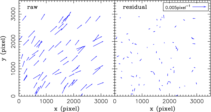
Figure 5: The spin-1 PSF anisotropy field $\zeta^{obs}_{*}(x,y)$ before (left) and after (right) the PSF correction over the Subaru $i^{\prime}$-band image of A1689. The spin-1 PSF anisotropy was measured from stellar shape moments following the HOLICs formalism outlined in §3. The orientation of the vectors shows the direction of the spin-1 anisotropy, and the length is proportional to the magnitude of anisotropy. A vector of $0.005{\rm pixel}^{-1}$ is displayed in the inset panel.

We used our weak lensing analysis pipeline based on IMCAT (Kaiser et al. 1995) extended to include our HOLICs moment method. We selected a stellar sample of $N_{*}=73$ objects for measuring the anisotropic/isotropic PSF effects. On the basis of the simulation results, we excluded from our background galaxy sample those small objects whose half-light radius ($r_{h}$) and Gaussian detection radius ($r_{g}$) are smaller than or comparable to the PSF; here we selected galaxies with $0\farcs 6<r_{h}<2^{\prime\prime}$ and $r_{g}>0\farcs 38$, whereas the median values of stellar $r_{h}$ and $r_{g}$ are $\langle r_{h*}\rangle\approx 0\farcs 48$ and $\langle r_{g*}\rangle\approx 0\farcs 34$ using $N_{*}=73$ stars. These lower cutoffs in the galaxy size are essential for reliable flexion measurements, because the smaller the object, the noisier its shape measurement due to pixelization noise; and the shape of an image whose intrinsic size is smaller than or comparable to the PSF size can be highly distorted and smeared, as we have seen in §5.1. Faint objects will also yield noisy shape measurements, in particular for the case of higher order shape moments. We thus selected bright galaxies with $20<i^{\prime}<25$ in the AB magnitude system. Further we excluded from our background sample those objects whose flexion estimates are significantly larger than the model prediction ($|F|\sim 0.1$ arcsec^-1) using the best-fitting NFW profile derived from the joint Subaru and ACS analysis (Broadhurst et al. 2005a); with this model, we set an upper cutoff in flexion of $|F|<0.4$ arcsec^-1, and an upper cutoff in the first HOLICs of $|\zeta^{iso}|<0.03$ arcsec^-1 (see equation [88]). We note that the measurements of spin-3 HOLICs $\delta$ were found to be quite noisy (see OUF for detailed discussions), so that we discarded the second flexion measurements from the present study. Finally, these selection criteria yielded a sample of $791$ galaxies usable for our flexion analysis, corresponding to a mean surface number density of $\bar{n}_{g}=7.75$ arcmin^-2. Using the background galaxy sample above we found a mean value of $\langle F\rangle=0.000223$ arcsec^-1 and a dispersion of $\sigma_{F}=0.11245$ arcsec^-1. In Figure 5 we show the spatial distribution of spin-1 PSF anisotropy as measured from stellar images before (left panel) and after (right panel) the anisotropic PSF correction. Figure 6 compares the distribution of two components of complex spin-1 PSF anisotropy before (left panel) and after(right panel) the anisotropic PSF correction. As clearly shown in Figures 5 and 6, the higher-order PSF anisotropy in observational data is indeed significant, so that one needs to take into account the higher-order PSF anisotropy correction in practical flexion measurements.

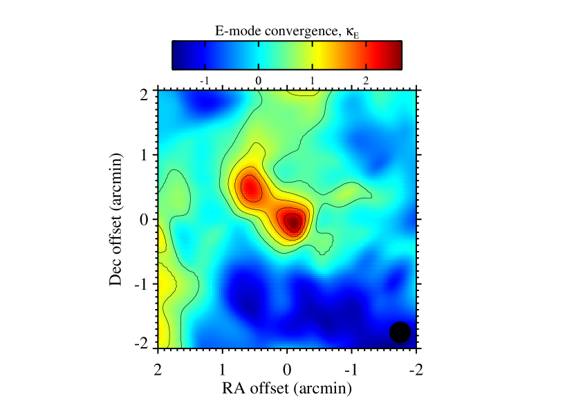
Figure 7: The dimensionless surface mass density $\kappa$ of the galaxy cluster A1689 ($z=0.183$) in the central $4^{\prime}\times 4^{\prime}$ region reconstructed using the first flexion observed with Subaru telescope/Suprime-Cam. The lowest contour and the contour interval are at a $1\sigma$ level of the reconstruction error ($\approx 0.51$) estimated from the rms of the $B$-mode reconstruction. The black, solid circle in the lower-right corner indicates the Gaussian FWHM ($=0\farcm 33$) used for the mass reconstruction.

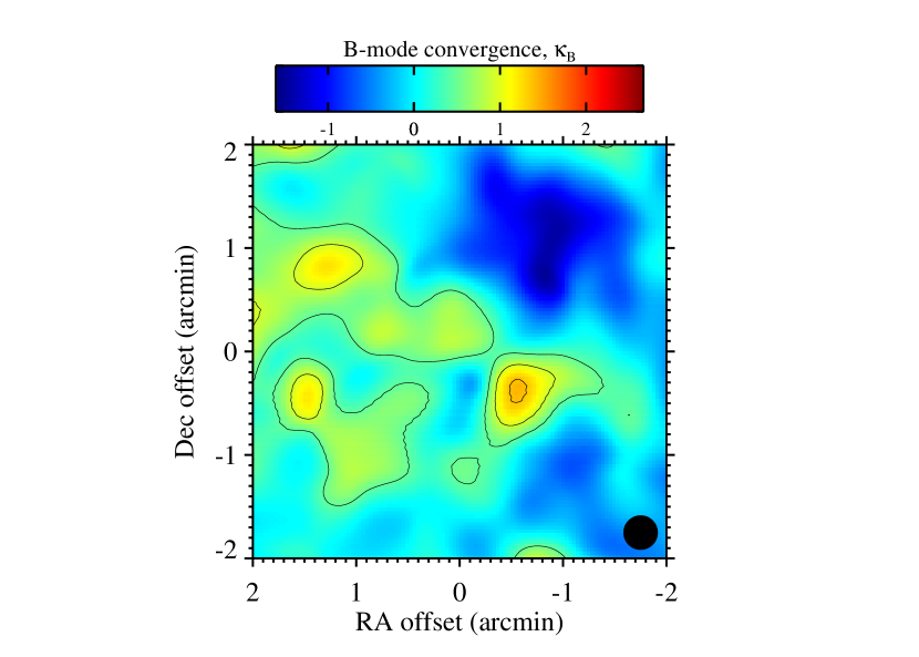
Figure 8: Same as Figure 7 but for the B-mode reconstruction from the first flexion measured from Subaru data. The color scale is the same as in Figure 7. The lowest contour and the contour interval are at a $1\sigma$ level of the B-mode reconstruction ($\sigma_{B}\approx 0.51$) over the $8^{\prime}\times 8^{\prime}$ region.

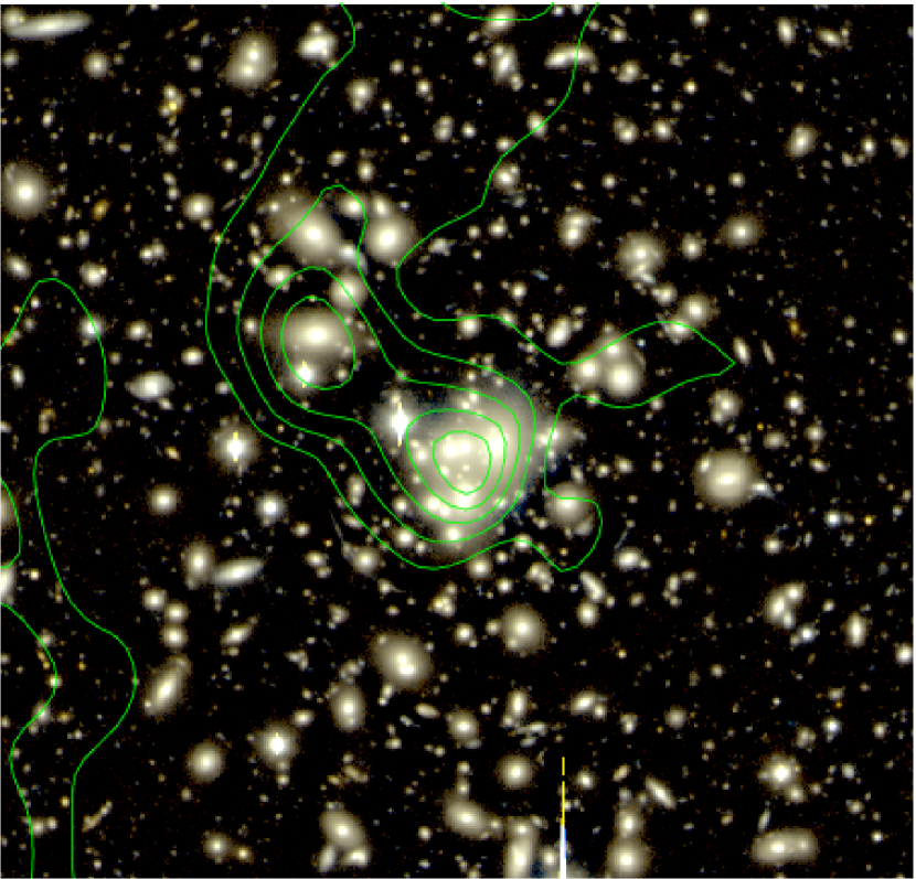
Figure 9: False-color image of the central $4^{\prime}\times 4^{\prime}$ cluster region composed of the Subaru/Suprime-Cam $V$ and $i^{\prime}$ images. Overlayed are contours of the lensing $\kappa$-field reconstructed from the first flexion measurements using the $i^{\prime}$-band data. The contours are spaced in units of $1\sigma(\approx 0.51)$ reconstruction error estimated from the rms of the $B$-mode reconstruction. North is to the top, and East to the left.

We use our first flexion measurements obtained with our moment-based analysis method to reconstruct the projected mass distribution of A1689. To do this we utilize the Fourier-space relation between the first flexion $F$ and the lensing convergence $\kappa$ (§2.4 of OUF; Bacon et al. 2006) with the weak lensing approximation. The field size for the mass reconstruction is $9^{\prime}\times 9^{\prime}$, sampled with a grid of $256\times 256$ pixels, over which the unconstrained $k=0$ mode is set to zero. Figures 7 and 8 show the $E$-mode convergence $\kappa=\kappa_{E}$ due to lensing and the $B$-mode convergence $\kappa_{B}$ which is expected to vanish in the weak lensing limit and can thus be used to monitor the reconstruction error in the $E$-mode $\kappa$ map. A central $8^{\prime}\times 8^{\prime}$ region is displayed in Figures 7 and 8. The reconstructed $\kappa$ maps were smoothed with a Gaussian filter of ${\rm FWHM}=0\farcm 33$. Table 1 lists basic statistics of the reconstructed $E$- and $B$-mode $\kappa$ fields measured in the central $8^{\prime}\times 8^{\prime}$ field. The rms dispersion in the Gaussian smoothed $B$-mode $\kappa$ map is obtained as $\sigma_{B}\approx 0.51$. The maximum and minimum values in the $B$-mode convergence field are $1.52$ and $-1.61$, corresponding to $2.9\sigma$ and $-3.1\sigma$ fluctuations (see Table 1). Figure 7 reveals two significant mass concentrations in the $E$-mode $\kappa$ map associated with clumps of bright galaxies. The first peak has a peak value of $\kappa_{E}=2.66$, and is detected at $5.2\sigma$ significance. This first peak is associated with the central concentration of bright cluster galaxies including the cD galaxy, as shown in Figure 9. This central mass concentration associated with the brightest cluster galaxies was not detected in the earlier ACS flexion analysis by Leonard et al. (2007). The ACS/Subaru best-fitting NFW model predicts $\kappa(z_{s}=1)\approx 2.5$ at $\theta\sim 0\farcm 1$. The second peak ($4.4\sigma$ significance), on the other hand, is located $\approx 0\farcm 9$ to the northeast direction, and is associated with a local clump of bright galaxies (see Figure 9), having a peak value of $\kappa_{E}=2.23$. This second mass peak has been detected in the earlier lensing studies based on the high resolution HST/ACS data (e.g, Broadhurst et al. 2005b; Leonard et al. 2007), and its likely bimodality in the central region has been discussed previous studies (Miralda-Escude & Babul 1995; Halkola, Seitz, & Pannella 2006; Limousin et al 2007; Saha, Williams, & Ferreras 2007). However, as compared to the Subaru weak lensing analysis by Umetsu & Broadhurst (2007), the flexion-based mass reconstruction cannot recover the global cluster structure on larger angular scales ($\;\buildrel>\over{\sim}\;$ a few arcmin), as demonstrated by OUF.

6 Discussion and Conclusions

In the present paper, we have developed a method for weak lensing flexion analysis by fully extending the KSB method to include the measurement of HOLICs (OUF). In particular, we take into account explicitly the weight function in calculations of noisy shape moments and the effects of spin-1 and spin-3 PSF anisotropies, as well as isotropic PSF smearing, in the limit of weak lensing and small PSF anisotropy ($q$). The higher order weak lensing effect induces a centroid shift in the observed image of the background (Goldberg & Bacon 2005; OUF; Goldberg & Leonard 2007). In weighted moment calculations, this will yield in the flexion measurement additional correction terms (relevant to $W^{\prime}(x),W^{\prime\prime}(x),W^{\prime\prime\prime}(x)$) that must be taken into account by properly expanding the weight function $W(x)$. It is found that neglecting these additional terms originated from the Taylor expansion of $W(x)$ yields the same result as obtained by Goldberg & Leonard (2007; see Appendix therein). We extended the KSB formalism to include the higher-order isotropic and anisotropic PSF effects relevant to spin-1 and spin-3 HOLICs by following the prescription given by KSB and Bartelmann & Schneider (2001), which provides direct relations between the observable HOLICs and underlying flexion in the weak lensing limit.

We have implemented in our analysis pipeline our flexion analysis algorithm based on the HOLICs moment approach, and tested the reliability and limitation of our PSF correction scheme using numerical simulations. Our simulation results show that (i) after applying our PSF correction method the PSF-induced anisotropies in HOLICs of mock galaxy images can be considerably reduced by a factor of $10$–$100$, depending on the strength of PSF anisotropy, (ii) those small galaxies whose angular size is smaller than or comparable to the size of PSF suffer from severe anisotropic PSF effects, and that (iii) there is an overall trend that the fractional correction factor is larger for larger galaxy images. Therefore, our simulation results support the reliability of our PSF-correction scheme and its practical implementation.

Based on the simulation results, we have applied our flexion analysis pipeline to ground-based $i^{\prime}$ imaging data of the rich cluster A1689 ($z=0.183$) taken with Subaru/Suprime-Cam. Our flexion analysis of Subaru A1689 data revealed a non-negligible, significant effect of higher-order PSF anisotropy induced in stellar images (Figures 5 and 6). It is therefore important in practical flexion measurements to quantify and correct for the higher-order anisotropic PSF effects.

Our mass reconstruction from the first-flexion measurements shows two significant ($>4\sigma$) mass structures associated with concentrations of bright galaxies in the central cluster region: the first peak ($5.2\sigma$) associated with the central concentration of bright galaxies including the cD galaxy, and the second peak ($4.4\sigma$) associated with a clump of bright galaxies located $\sim 1^{\prime}$ northeast of the cluster center. This significant detection of the second peak confirms earlier ACS results from the strong lensing analysis (Broadhurst et al. 2005b; Halkola et al. 2006; Leonard et al. 2007) and the combined strong lensing, weak shear, and flexion analysis by Leonard et al. (2007). The central mass peak, however, was not recovered in the earlier flexion analysis by Leonard et al. (2007) based on HST/ACS data. Leonard et al. (2007) attributed this to their relatively large reconstruction error at the cluster center, although they have a very large number density of background galaxies, $\bar{n}_{g}\approx 75$ arcmin^-2. On the other hand, owing to our conservative selection criteria for the background sample, the mean number density of background galaxies used for the present analysis is $\bar{n}_{g}=7.75$ arcmin^-2, which is almost one order of magnitude smaller than that of the ACS data, and is about $20\%-30\%$ of a typical number density of magnitude/size-selected background galaxies usable for the quadrupole shape measurements in ground-based Subaru observations ($\bar{n}_{g}\sim 30-40{\rm arcmin}^{-2}$). However, we found that it is rather important to remove small/faint galaxy images and noisy outliers in flexion measurements since they are likely to be affected by the residual PSF anisotropy and/or observational noise in the shape measurement (§5.1). Besides, the smaller the object, the larger the amplitude of intrinsic flexion contributions. Recall that flexion and HOLICs have a dimension of length inverse: The response to flexion is size-dependent, and the amplitude of intrinsic flexion is inversely proportional to the object size. Indeed, we find that inclusion of smaller objects results in a noisy reconstruction. Similar values of the background number density, $\bar{n}_{g}\lower 2.15277pt\hbox{$\;\buildrel<\over{\sim}\;$}10{\rm arcmin}^{-2}$, have been used in recent quadrupole weak lensing analyses based on Subaru observations (e.g., Broadhurst et al. 2005a; Umetsu & Broadhurst 2007; weak lensing cluster mass measurements of Okabe & Umetsu 2008). In their studies only objects redder than the cluster sequence are selected in color-magnitude space for their weak lensing analysis, because such a red population is expected to comprise only background galaxies ($\bar{z}_{s}\sim 0.9$; see, e.g., Medezinski et al. 2007), made redder by relatively large $k$-corrections and with negligible contamination by cluster galaxies (Broadhurst et al. 2005a; Medezinski et al. 2007). However, the smaller number of objects implies a coarser angular resolution in the map-making for achieving a proper signal-to-noise ratio (e.g., per-pixel ${\rm S/N}\lower 2.15277pt\hbox{$\;\buildrel>\over{\sim}\;$}1$). With $\bar{n}_{g}\sim 10{\rm arcmin}^{-2}$ for cluster quadrupole weak lensing, typical angular resolutions are about $1-2$ arcmin (e.g., Gaussian FWHM, or boxcar width). On the other hand, flexion measures essentially the gradient of the tidal gravitational shear field (i.e., $F,G\propto\phi(r)/r^{3}$), and hence is relatively sensitive to small-scale structures. Therefore, our successful reconstruction of the mass substructures with a small background density, $\bar{n}_{g}\sim 8{\rm arcmin}^{-2}$, could be attributed to the superior sensitivity of flexion to small scale structures (see OUF for detailed discussions) and the here-adopted selection criteria for a background galaxy sample for weak lensing flexion analysis.

Finally, we emphasize that our HOLICs formalism here is different from the earlier work by Goldberg & Leonard (2007) in that (1) additional correction terms for the centroid shift, relevant to the derivatives of the weight function, have been included and (2) the spin-1 and spin-3 PSF anisotropies, as well as the isotropic PSF smearing, have been taken into account under the assumption of small PSF anisotropy ($q[\mbox{\boldmath$\theta$}]$), as done in the KSB formalism. Our flexion-based mass reconstruction of A1689 demonstrates the power of the generalized flexion analysis techniques for quantitative and accurate measurements of the weak gravitational lensing effects.

Appendix A HOLICs Formalism in the Complex Form

A.1 Complex Displacement

In this Appendix, we adopt the following notations to represent complex quantities with the degree $N$ and the spin number $M$:

$$X^{N}_{M} \equiv (\Delta\theta_{1}+i\Delta\theta_{2})^{\frac{N+M}{2}}(\Delta\theta_{1}+i\Delta\theta_{2})^{*\frac{N-M}{2}}$$ (A1)

$$= (\Delta\theta_{1}+i\Delta\theta_{2})^{\frac{N+M}{2}}(\Delta\theta_{1}-i\Delta\theta_{2})^{\frac{N-M}{2}},$$

$$Y^{N}_{M} \equiv (\Delta\beta_{1}+i\Delta\beta_{2})^{\frac{N+M}{2}}(\Delta\beta_{1}+i\Delta\beta_{2})^{*\frac{N-M}{2}}$$ (A2)

$$= (\Delta\beta_{1}+i\Delta\beta_{2})^{\frac{N+M}{2}}(\Delta\beta_{1}-i\Delta\beta_{2})^{\frac{N-M}{2}}.$$

Here a quantity with the spin number of $-M$ is equivalent to the complex conjugate of the corresponding spin-$M$ quantity. Unless otherwise noted, we shall use $X^{N}_{M}$ to represent complex quantities in the image plane, and $Y^{N}_{M}$ those in the source plane.

The product of $X^{N}_{M}$ and $X^{L}_{K}$ is expressed as

$$X^{N}_{M}X^{L}_{K} = X^{N+L}_{M+K},$$

$$X^{N}_{M}X^{L*}_{K} = X^{N+L}_{M-K}\ \ \ (M>K),$$ (A3)

$$= (X^{N*}_{M}X^{L}_{K})^{*}=\left(X^{N+L}_{K-M}\right)^{*}\ \ \ (M<K).$$

For arbitrary complex numbers $W$ and $Z$ the following identities hold:

$$2{\rm Re}\left[WX^{N*}_{M}\right]X^{L}_{K} = \left(WX^{N*}_{M}+W^{*}X^{N}_{M}\right)X^{L}_{K}=WX^{N+L}_{K-M}+W^{*}X^{N+L}_{M+K},$$ (A4)

$$4{\rm Re}\left[WX^{N*}_{M}\right]{\rm Re}\left[ZX^{L*}_{K}\right] = \left(WX^{N*}_{M}+W^{*}X^{N}_{M}\right)\left(ZX^{L*}_{K}+Z^{*}X^{L}_{K}\right),$$ (A5)

$$= WZ\left(X^{N+L}_{K+M}\right)^{*}+WZ^{*}X^{N+L}_{K-M}+W^{*}ZX^{N+L}_{-K+M}+W^{*}Z^{*}X^{N+L}_{K+M},$$

$$= 2{\rm Re}\left[WZ\left(X^{N+L}_{K+M}\right)^{*}\right]+2{\rm Re}\left[WZ^{*}X^{N+L}_{K-M}\right].$$

A.2 HOLICs Family

We summarize in the complex form a family of complex shape moments including HOLICs relevant to the weak lensing flexion analysis.

$$M =\int d^{2}\theta I(\theta)W(X^{2}_{0}/\sigma^{2}) {\rm(spin-0)}$$

$$D =\frac{\int d^{2}\theta I(\theta)W(X^{2}_{0}/\sigma^{2})X^{1}_{1}}{M} {\rm(spin-1)},$$

$${\rm tr}Q =\int d^{2}\theta I(\theta)W(X^{2}_{0}/\sigma^{2})X^{2}_{0} {\rm(spin-0)},$$

$$\chi =\frac{\int d^{2}\theta I(\theta)W(X^{2}_{0}/\sigma^{2})X^{2}_{2}}{{\rm tr}Q} {\rm(spin-2)},$$

$$\zeta =\frac{\int d^{2}\theta I(\theta)W(X^{2}_{0}/\sigma^{2})X^{3}_{1}}{\xi} {\rm(spin-1)},$$

$$\delta =\frac{\int d^{2}\theta I(\theta)W(X^{2}_{0}/\sigma^{2})X^{3}_{3}}{\xi} {\rm(spin-3)},$$

$$\xi ={\int d^{2}\theta I(\theta)W(X^{2}_{0}/\sigma^{2})X^{4}_{0}} {\rm(spin-0)},$$

$$\eta =\frac{\int d^{2}\theta I(\theta)W(X^{2}_{0}/\sigma^{2})X^{4}_{2}}{\xi} {\rm(spin-2)},$$

$$\lambda =\frac{\int d^{2}\theta I(\theta)W(X^{2}_{0}/\sigma^{2})X^{4}_{4}}{\xi} {\rm(spin-4)},$$

$$\iota_{I} =\frac{\int d^{2}\theta I(\theta)W(X^{2}_{0}/\sigma^{2})X^{5}_{1}}{\xi} {\rm(spin-1)},$$

$$\iota_{III} =\frac{\int d^{2}\theta I(\theta)W(X^{2}_{0}/\sigma^{2})X^{5}_{3}}{\xi} {\rm(spin-3)},$$

$$\iota_{V} =\frac{\int d^{2}\theta I(\theta)W(X^{2}_{0}/\sigma^{2})X^{5}_{5}}{\xi} {\rm(spin-5)},$$

$$\upsilon_{0} =\int d^{2}\theta I(\theta)W(X^{2}_{0}/\sigma^{2})X^{6}_{0} {\rm(spin-0)},$$

$$\upsilon_{II} =\frac{\int d^{2}\theta I(\theta)W(X^{2}_{0}/\sigma^{2})X^{6}_{2}}{\xi} {\rm(spin-2)},$$

$$\upsilon_{IV} =\frac{\int d^{2}\theta I(\theta)W(X^{2}_{0}/\sigma^{2})X^{6}_{4}}{\xi} {\rm(spin-4)},$$

$$\upsilon_{VI} =\frac{\int d^{2}\theta I(\theta)W(X^{2}_{0}/\sigma^{2})X^{6}_{6}}{\xi} {\rm(spin-6)},$$

$$\tau_{I} =\frac{\int d^{2}\theta I(\theta)W(X^{2}_{0}/\sigma^{2})X^{7}_{1}}{\xi} {\rm(spin-1)},$$

$$\tau_{III} =\frac{\int d^{2}\theta I(\theta)W(X^{2}_{0}/\sigma^{2})X^{7}_{3}}{\xi} {\rm(spin-3)},$$

$$\tau_{V} =\frac{\int d^{2}\theta I(\theta)W(X^{2}_{0}/\sigma^{2})X^{7}_{5}}{\xi} {\rm(spin-5)},$$

$$\tau_{VII} =\frac{\int d^{2}\theta I(\theta)W(X^{2}_{0}/\sigma^{2})X^{7}_{7}}{\xi} {\rm(spin-7)}.$$ (A6)

A.3 Differential Operators

Let us first define the complex gradient operator $\partial$ as

$$\partial=\left(\frac{\partial}{\partial\theta_{1}}+i\frac{\partial}{\partial\theta_{2}}\right).$$ (A7)

Operating $\partial$ on complex $X^{N}_{M}$ yields:

$$\partial X^{1}_{1} =\left(\frac{\partial}{\partial\theta_{1}}+i\frac{\partial}{\partial\theta_{2}}\right)(\theta_{1}+i\theta_{2})=(1-1)=0,$$ (A8)

$$\partial^{*}X^{1}_{1} =\left(\frac{\partial}{\partial\theta_{1}}-i\frac{\partial}{\partial\theta_{2}}\right)(\theta_{1}+i\theta_{2})=(1+1)=2,$$

$$\partial X^{N}_{M} =\partial\left(\left(X^{1}_{1}\right)^{\frac{N+M}{2}}\left(X^{1*}_{1}\right)^{\frac{N-M}{2}}\right)=(N-M)\left(X^{1}_{1}\right)^{\frac{N+M}{2}}\left(X^{1*}_{1}\right)^{\frac{N-M-2}{2}}=(N-M)X^{N-1}_{M+1},$$

$$\partial^{*}X^{N}_{M} =\partial^{*}\left(\left(X^{1}_{1}\right)^{\frac{N+M}{2}}\left(X^{1*}_{1}\right)^{\frac{N-M}{2}}\right)=(N+M)\left(X^{1}_{1}\right)^{\frac{N+M-2}{2}}\left(X^{1*}_{1}\right)^{\frac{N-M}{2}}=(N+M)X^{N-1}_{M-1}.$$ (A9)

Similarly, by operating $\partial$ on the weight function $W(X_{0}^{2}/\sigma^{2})$, one finds the following:

$$\partial W\left(\frac{X^{2}_{0}}{\sigma^{2}}\right) = \frac{2}{\sigma^{2}}X^{1}_{1}W^{\prime}\left(\frac{X^{2}_{0}}{\sigma^{2}}\right),$$

$$\partial^{*}W\left(\frac{X^{2}_{0}}{\sigma^{2}}\right) = \frac{2}{\sigma^{2}}X^{1*}_{1}W^{\prime}\left(\frac{X^{2}_{0}}{\sigma^{2}}\right),$$ (A10)

where $F$ and $G$ are the first and the second flexion defined as $F={\cal F}/(1-\kappa)$ and $G={\cal G}/(1-\kappa)$, respectively. Then, the complex displacement in the source plane, $\Delta\beta$, is expressed in terms of the lensing convergence, shear and flexion as

$$\Delta\beta=\Delta\beta_{1}+i\Delta\beta_{2}\equiv Y^{1}_{1}\approx(1-\kappa)\left[X^{1}_{1}-gX^{1*}_{1}-\frac{1}{4}\left(2FX^{2}_{0}+F^{*}X^{2}_{2}+GX^{2*}_{2}\right)\right].$$ (A11)

The integration measures in the source and image planes are related in the following way

$$d^{2}\beta = (1-\kappa)^{2}\Biggl{(}1-2{\rm Re}\left[FX^{1*}_{1}\right]-|g|^{2}+\frac{1}{4}|F|^{2}X^{2}_{0}-\frac{1}{4}|G|^{2}X^{2}_{0}$$ (A12)

$$+ \frac{1}{2}{\rm Re}\left[F^{2}X^{2*}_{2}\right]-{\rm Re}\left[g^{*}FX^{1}_{1}\right]-{\rm Re}\left[g^{*}GX^{1*}_{1}\right]-\frac{1}{2}{\rm Re}\left[FG^{*}X^{2}_{2}\right]\Biggr{)}d^{2}\theta$$

$$\approx (1-\kappa)^{2}\left(1-2{\rm Re}\left[FX^{1*}_{1}\right]\right)d^{2}\theta,$$

to the first order of reduced flexion (e.g. OUF).

Table 1: Basic statistics of the reconstructed $E$ and $B$ mode convergence fields

field	mean ($\bar{\kappa}$)	$\sigma$	skewness	kurtosis	minimum	maximum
$B$	0.058	0.512	$-0.334\pm 0.2$	$0.043\pm 0.4$	-1.61	1.52
$E$	-0.058	0.701	$-0.239\pm 0.2$	$0.125\pm 0.4$	-2.09	2.66

Note. — The moments are calculated from the convergence within the central $8^{\prime}\times 8^{\prime}$ region.

Figure 1: Test of anisotropic PSF correction for the first HOLICs of spin-1, $\zeta$, based on numerical simulations. No observational noise and lensing signal is included. The values of first HOLICs multiplied with the object detection radius, $r_{g}|\zeta|$, are shown as a function of parameters $A_{\rm aniso}$ (left: $\theta_{\rm aniso}=0.92\sigma_{iso}$) and $\theta_{\rm aniso}$ (right: $A_{\rm aniso}=0.1$) for a model PSF anisotropy. Solid lines indicate the observed values of first HOLICs ($\zeta^{obs}$) for Gaussian source images smeared with the model PSF, and dashed lines indicate the residual values ($\zeta^{iso}$) after correcting for the spin-1 PSF anisotropy. No observational noise or lensing signal has been added. The PSF consists of an isotropic part $P^{iso}$ described by a truncated Gaussian with dispersion $\sigma_{iso}$ and an isotropic part $q(\theta)=A_{aniso}\theta_{1}/|\mbox{\boldmath$\theta$}|^{2}$ truncated at $\theta=\theta_{aniso}$. Filled circles, open triangles, and crosses represent the measurements for a Gaussian source of dispersion $R_{\rm gal}=1\sigma_{iso},2\sigma_{iso},3\sigma_{iso}$, respectively. The $\zeta_{obs}$ is measured with a Gaussian weight function of dispersion $r_{g}=\sqrt{R_{\rm gal}^{2}+\sigma_{iso}^{2}}$ from the surface brightness distribution smeared with the model PSF.

Figure 2: Ratio of residual to observed spin-1 PSF anisotropy, $|\zeta^{iso}|/|\zeta^{obs}|$, as a function of model parameters $A_{\rm aniso}$ (left) and $\theta_{\rm aniso}$ (right) for the PSF anisotropy kernel. The PSF consists of an isotropic part $P^{iso}$ described by a truncated Gaussian with dispersion $\sigma_{iso}$ and an isotropic part $q(\theta)=A_{aniso}\theta_{1}/|\mbox{\boldmath$\theta$}|^{2}$ truncated at $\theta=\theta_{aniso}$. Filled circles, open triangles, and crosses represent the measurements for a Gaussian source of dispersion $R_{\rm gal}=1\sigma_{iso},2\sigma_{iso},3\sigma_{iso}$, respectively.

Figure 3: Same as Figure 1 but for the second HOLICs, $\delta$, of spin-3.

Figure 4: Same as Figure 2 but for the second HOLICs, $\delta$, of spin-3.

Figure 6: Comparison of spin-1 PSF anisotropy components before (left) and after (right) the PSF correction.

References

• (1) Bacon, D. J., Refregier, A. R., Ellis, R. S. 2000, MNRAS, 318, 625
• (2) Bacon, D. J., Goldberg, D. M., Rowe, B. T. P., & Taylor, A. N. 2006, MNRAS, 365, 414
• (3) Bardeau, S. et al. 2005 A&A, 434, 433
• (4) Bartelmann, M., & Schneider, P. 2001, Phys.Rep., 340, 291 652, 937.
• (5) Broadhurst, T., Taylor, A. N., & Peacock, J. A. 1995, ApJ, 438, 49
• (6) Broadhurst, T. et al. 2005, ApJ, 621, 53 (Broadhurst et al. 2005b)
• (7) Broadhurst, T., Takada, M., Umetsu, K., Kong, X., Arimoto, N., Chiba, M., & Futamase, T. 2005, 619, 143L (Broadhurst et al. 2005a)
• (8) Bullock, J. S. et al. 2001, MNRAS, 321, 559
• (9) Erben, T. et al. 2000, A&A, 355, 23
• (10) Goldberg, D. M. & Natarajan, P. 2002, ApJ, 564, 65
• (11) Goldberg, D. M., & Bacon, D. J. 2005, ApJ, 619, 741
• (12) Goldberg, D. M., & Leonard, A. 2006, ApJ, 660, 1003
• (13) Halkola, A. Seitz, S., & Pannella, M. 2006, MNRAS, 372, 1425
• (14) Hamana, T. et al. 2003, ApJ, 597, 98
• (15) Heymans, C. et al. 2006, MNRAS, 368, 1323
• (16) Irwin, J., & Shmakova, M. 2006, ApJ, 645, 17
• (17) Kaiser, N., & Squires, G. 1993, ApJ, 404, 441
• (18) Kaiser, N., Squires, G., Broadhurst, T. 1995, ApJ, 449, 460
• (19) King, L. J., Clowe, D. I., Schneider, P. 2002 A&A, 383, 118
• (20) Leonard, A., Goldberg, D. M., Haaga, J. L., Massey, R. 2007, ApJ, 666, 51L
• (21) Medezinski, E., Broadhurst, T., Umetsu, K., Coe, D., Benitez, N., Ford, H., Rephaeli, Y., Arimoto, N., & Kong, X. 2007, ApJ, 663, 717
• (22) Limousin, M. et al. 2007, ApJ, 668, 643
• (23) Massey, R. et al. 2007, MNRAS, 376, 13
• (24) Navarro, J. F., Frenk, C. S., White, S. D. M., 1997, ApJ, 490, 493
• (25) Neto, A. F. et al. 2007, MNRAS, 381, 1450
• (26) Okabe, N. & Umetsu, K. 2008, PASJ, in press (arXiv:astro-ph/0702649)
• (27) Okura, Y., Umetsu, K., & Futamase, T. 2007, ApJ, 660, 995
• (28) Refregier, A. 2003, MNRAS, 338, 35
• (29) Saha, P., Williams, L. L. R., Ferreras, I. 2007, ApJ, 663, 29
• (30) Schneider, P. & Seitz, C. 1995, A&A294, 411
• (31) Schneider, P. & Er, X. 2007, submitted to A&A (astro-ph/0709.1003)
• (32) Tyson, J. A., & Fisher, P., 1995 ApJ 446 L55
• (33) Umetsu, K, Tada, M., & Futamase, T. 1999, Prog. Theor. Phys. Suppl., 133, 53
• (34) Umetsu, K, & Futamase, T. 2000, ApJ, 539, L5
• (35) Umetsu, K., Takada, M., Broadhurst, T. 2007, Mod. Phys. Lett. A, 22, 2099 (arXiv:astro-ph/0702096)
• (36) Umetsu, K. & Broadhurst, T. 2007, submitted to ApJ (arXiv:astro-ph/0712.3441)
• (37) Van Waerbeke et al. 2001, A&A, 374, 757
• (38) Wittman, D. et al. 2001, ApJ, 557, 89L