High-energy neutrinos in the context of multimessenger astrophysics
Abstract
The field of astroparticle physics is currently developing rapidly, since new experiments challenge our understanding of the investigated processes. Three messengers can be used to extract information on the properties of astrophysical sources: photons, charged Cosmic Rays and neutrinos. This review focuses on high-energy neutrinos ( GeV) with the main topics as follows.
-
•
The production mechanism of high-energy neutrinos in astrophysical shocks. The connection between the observed photon spectra and charged Cosmic Rays is described and the source properties as they are known from photon observations and from charged Cosmic Rays are presented.
-
•
High-energy neutrino detection. Current detection methods are described and the status of the next generation neutrino telescopes are reviewed. In particular, water and ice Cherenkov detectors as well as radio measurements in ice and with balloon experiments are presented. In addition, future perspectives for optical, radio and acoustic detection of neutrinos are reviewed.
-
•
Sources of neutrino emission. The main source classes are reviewed, i.e. galactic sources, Active Galactic Nuclei, starburst galaxies and Gamma Ray Bursts. The interaction of high energy protons with the cosmic microwave background implies the production of neutrinos, referred to as GZK neutrinos.
-
•
Implications of neutrino flux limits. Recent limits given by the AMANDA experiment and their implications regarding the physics of the sources are presented.
keywords:
Astrophysical neutrinos , Neutrino telescopes , multimessenger astrophysics , AGN , GRBs , Cosmic RaysPACS:
13.85.Rm, 95.55.Ym, 98.54.Cm, 13.15+g, 13.85.Tp , 95.30.Cq1 Introduction
The multimessenger connection between Cosmic Rays, photons and neutrinos of different wavelengths is crucial to comprehend in the pursuit of a deeper understanding of the fundamental processes driving non-thermal astrophysical sources. None of these messengers alone is able to give a complete picture. While photons reveal the surface of those objects due to the optical thickness of the sources, charged Cosmic Rays give a direct sight into the inner acceleration processes. However, they do not point back to their origin, since scrambled by intergalactic magnetic fields. Neutrinos are produced in interactions of protons with a photon field or other protons. The detection of an extraterrestrial neutrino signal at the highest energies ( GeV) renders possible the exploration of the particle acceleration region itself. Neutrinos escape the acceleration region and propagate through space basically untouched and this advantage is directly connected to the drawback of the very low detection probability of neutrinos. In this review, the connection of the three messengers will be reviewed with the focus on the resulting neutrino fluxes and their detection probabilities.
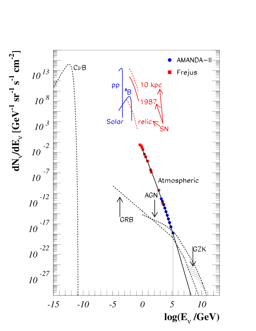
Astrophysical neutrinos are produced over the broad energy range, covering 15 orders of magnitude. An overview of the neutrino spectrum is shown in Fig. 1. From the lowest energies of meV to the highest energies of EeV, the intensity of the signal decreases by 42 orders of magnitude, making it necessary to introduce new methods of neutrino detection and analysis in order to increase the sensitivity to the neutrino fluxes especially at the highest energies.
The Cosmic Neutrino Background (CB) is an isotropic neutrino flux having decoupled in the early Universe, only s after the Big Bang, see Wei (72) and references therein. It is the neutrino equivalent of the cosmic microwave background (CMB). The temperature of the blackbody spectrum has dropped to K today due to the expansion of the Universe, and the flux peaks at milli-eV energies. While this background is essentially predicted in the standard model of cosmology, it was not possible to test it experimentally yet. Recently, the measurement of the CB was proposed by using the interaction of cosmic neutrinos with nuclei undergoing beta decay CMM (07), with 3H as an optimal candidate. For the case of a g 3H-detector, an event rate of a few tens to a few hundreds is expected. The exact number depends on the distribution of cosmic neutrinos and the neutrino mass. This is currently not within experimental reach, but can probably explored in the future with improved experimental techniques.
The sun emits neutrinos in different fusion processes in the MeV range. In the figure, neutrinos from interactions and the 7B spectrum is shown. Massive stars () are expected to emit neutrinos at MeV due to Silicon burning OMK (04); MOK (06).
At slightly higher energies lies the neutrino spectrum from SN 1987A. The expected flux from a SN at a distance of kpc is indicated. Such a close supernova will be observed by todays neutrino telescopes. The total diffuse flux from SNRs (“relic”), however, is about four orders of magnitude lower and could not be tested yet.
At energies of GeV, the measured spectrum of atmospheric neutrinos is indicated, squares are measurements from Fréjus B+ (87); D+ (95) and dots are AMANDA measurements from the years 2000-2003 M+ (07); Mün (07). At the highest energies, a generic spectrum from GRBs is indicated WB (97, 99), as well as the maximum contribution from AGN MPR (01) and the expected neutrino flux from the absorption of protons by the GZK effect YT (93). These sources have not been observed yet due to the high atmospheric background and limited sensitivities of the detectors. During the past ten years, high-energy neutrino detection still succeeded in improving the instruments in a way that made it possible to cover five decades of energy and to improve the sensitivity by 17 (seventeen!) orders of magnitude. We have today reached the point where the most optimistic models could already be used to constrain the physics of different sources classes and where the more realistic models are being challenged by the upcoming generation of neutrino detectors. This review discusses their options and possibilities.
In particular, the different source types being able to accelerate neutrinos to the highest energies are examined in more detail. The hypothesis of neutrino emission from these objects is reviewed quantitatively in the context of multimessenger physics. Section 3 focuses on what is known about the non-thermal Universe from photons and charged Cosmic Rays. The connection from these two messengers to the third, complementary particle, the neutrino, is drawn. In Section 4, the focus lies on the methods used to detect neutrinos at the highest energies. What neutrino signal to expect from extragalactic sources is considered in the following sections. Possible neutrino emission from galactic sources is presented in Section 5. Active Galactic Nuclei (AGN) are reviewed in Section 6, the neutrino flux models from Gamma Ray Bursts (GRBs) are discussed in Section 7 and starburst galaxies are presented in Section 8. Finally, production scenarios of neutrinos generated by the interaction of high-energy protons with the CMB are presented in Section 9 before closing with a summary in Section 10.
2 Introductory notes
2.1 On the representation of flux models in figures
Figure 1 shows the neutrino flux models in a double-logarithmic representation, implying that the dependence of the differential flux with the energy is shown as . In general, non-thermal particle spectra can usually be approximated by powerlaws, . In a double-logarithmic representation, this leads to a straight line,
The slope of the line is given by the spectral index and the y-axis intercept represents the normalization . Such powerlaw spectra are observed in the case of photons and charged Cosmic Rays, and are expected in the case of neutrinos. In the following, all spectra will be shown in the double-logarithmic representation. Since many spectra are very steep () for all three messengers, it is useful to weight the y-axis with a power of the energy, , straight line,
For , which is often used in the case of neutrino spectra, an -spectrum is then represented by a flat line, which is convenient, since neutrino spectra at GeV are often expected to be close to . The double-logarithmic representation with a weight is chosen to simplify to read off the spectral index of the models and measured fluxes.
2.2 Flux and limit notations
Throughout this review, different fluxes and flux limits will appear. Usually, the flux at Earth is given per energy interval, , in units of . Point source fluxes have the same notation, but the unit . The convention for the different particle and electromagnetic fluxes is as follows:
-
•
Charged Cosmic Rays
For the total spectrum of charged particles, the spectrum is written as(2) If only protons or electrons are considered, the following notation is used:
(3) -
•
Photons
Photon spectra are usually given as:(4) The total power , depending on the angular frequency , is written as
(5) with .
For the special case of TeV photons, the notation
(6) is used. The spectrum is normalized at 1 TeV.
-
•
Neutrinos
The neutrino spectrum is usually multiplied by the energy squared, ,(7) Alternatively, the spectrum itself is given as
(8) with .
Neutrino flux limits are usually given in the form of and are denoted as follows:
-
•
: Diffuse Limit (DL) given in units of .
-
•
: Stacking Limit (SL) in units of , obtained for the point source flux from a certain class of AGN. The stacking method is explained in Section 4.
-
•
: Stacking Diffuse Limit (SDL), derived from the stacking limit in the same units as the diffuse limit, . It is determined by taking into account the contribution from weaker sources as well as yet unidentified sources, present in a diffuse background.
A similar convention is used to denote the corresponding sensitivities:
-
•
: Diffuse Sensitivity (DS) in units of .
-
•
: the sensitivity to a single point source in units of .
3 The multimessenger connection
Neutrino flux predictions are built on the direct connection between the observed Cosmic Ray spectrum and the non-thermal emission from astronomical sources. Here, it is reviewed how the different parts of the Cosmic Ray spectrum can be connected to the various objects and source classes and how this in turn leads to the production of neutrinos.
3.1 Cosmic Rays
Charged Cosmic Rays (CRs) have been observed from energies of eV up to eV. The spectrum is altered by the Solar wind for energies below about GeV, where is the charge of the nucleus. At higher energies, the energy spectrum follows a powerlaw with two, possibly three breaks. The powerlaw structure can in general be explained by shock acceleration in astrophysical sources. In this section, the observed spectrum with its features is discussed as well as the acceleration mechanism built on stochastic acceleration of test particles at magnetic field inhomogeneities in astrophysical shocks.
3.1.1 Observation of charged Cosmic Rays
Already in the early 20th century, it was discovered that the Earth is exposed to a continuous flux of charged particles from outer space, see e.g. Hes (12); Koh (13). Viktor Hess and others performed balloon flights proving that the ionization of the atmosphere increases with height. This contradicted the hypothesis that the flux of ionizing particles arises from radioactive matter in the Earth’s rocks exclusively.
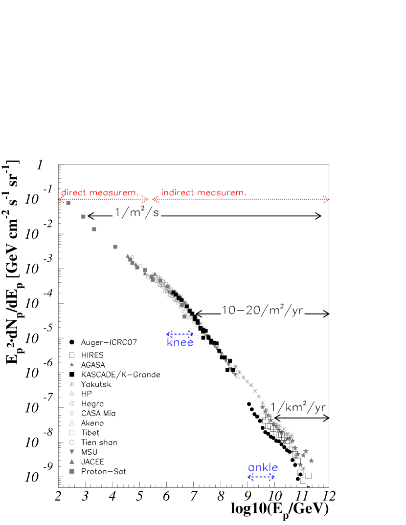
Today, the spectrum of charged CRs, , has been examined over a wide range of energies , using balloon experiments and satellites for low energies ( eV) and Earth-bound experiments for high energies ( eV). The all particle energy spectrum of CRs is shown in Fig. 2. The spectrum is weighted by in order to have a flatter representation of the very steep spectrum. The powerlaw behavior of the spectrum is clearly visible,
| (9) |
Two kinks can also be seen, referred to as knee and ankle. The spectral indices for the different parts of the spectrum are WBM (98); V+ (99)
| (10) |
A second knee around eV is discussed today, with an even steeper behavior up to the ankle, see e.g. Hör (03); HKT (07) and references therein. The general spectral powerlaw-like behavior can be explained by stochastic particle acceleration in collision-less plasmas.
Cosmic Rays & directional information
Charged Cosmic Rays below eV do not point back to their origin, since they are scrambled by interstellar magnetic fields. The strong connection between non-thermal emission from astrophysical sources and particle acceleration can, however, be used to establish a model for different sources and source types to explain the Cosmic Ray spectrum. Sources within our Galaxy can produce the Cosmic Ray spectrum up to the ankle. Events at higher energies have to be extragalactic:
-
(a)
no galactic source class is energetic enough for the production of particles at such high energies as discussed later in Section 3.1.2 and
-
(b)
the particles’ gyro-radius becomes too large and they escape from the galaxy already at lower energies.
-
(c)
In addition, at energies as high as eV, the particle diffusion is low compared to the traveling length through the Galaxy Hil (84). The observed particles point in this case back to their original source. The observed events are isotropically distributed, which is only possible for traveling lengths longer than the diameter of the galaxy.
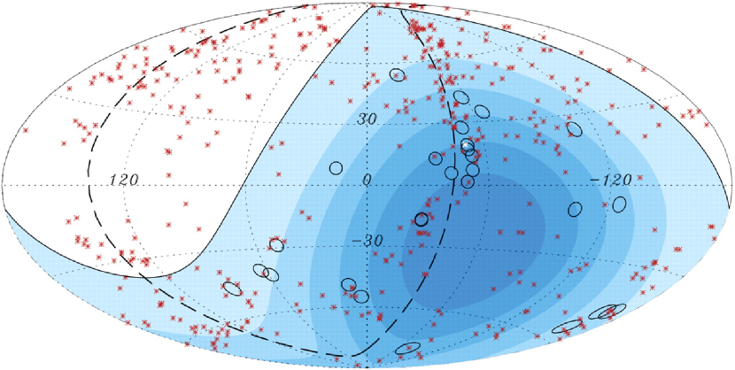
This leaves extragalactic or exotic sources as the origin of the highest energy events, for which acceleration up to eV is possible. At the highest observed energies, eV, nearby galaxies with distances smaller than Mpc can still carry directional information. At these distances, most galaxies are located in the supergalactic plane. Most recently, the Auger experiment observed a first evidence for the correlation between the Véron-Cetty (V-C) catalog of Active Galactic Nuclei and Cosmic Rays of the highest energies AA+07a . In the analysis, three parameters have been optimized in order to look for a correlation between the sources in the catalog and the events at the highest energies: The maximum angular separation between Cosmic Ray event and source, the maximum redshift for which AGN in the catalog are still considered and the threshold energy , giving the lowest energy at which Cosmic Ray events are still considered. These three parameters ensure that
-
(a)
magnetic deflection is considered to a certain amount ( is larger than the point spread function of the detector),
-
(b)
only the local Universe is considered (the choice of leaves out distant galaxies),
-
(c)
only events with the highest energies are considered. Events of energies below are discarded, since lower-energy events are more sensitive to magnetic field deflections.
The final parameter set is EeV, and the sky plot is shown in Fig. 3. The maximum redshift of corresponds to a distance of Mpc. The correlation is a first evidence that sources following the structure of the supergalacitc plane are the sources of the highest energy Cosmic Rays. The analysis does not allow for the direct identification of the sources for different reasons. Firstly, the catalog of AGN used in the analysis cannot considered to be complete and is partly inhomogeneous, including different types of AGN. Secondly, sources other than AGN, which also follow the local structure of the Universe, may be responsible for the emission of UHECRs rather than AGN themselves. Nonetheless, this result is a first step towards the identification of the sources of extragalactic Cosmic Rays.
The Greisen Zatsepin Kuzmin cutoff
Protons effectively lose energy by interactions with the CMB on their way to Earth:
| (11) |
The energy loss length for pair production at eV is about Mpc, while it is only Mpc for the production of a resonance. The latter process is therefore responsible for a rapid decrease of the particle spectrum above eV, if the sources of Cosmic Rays are located at distances larger than Mpc Gre (66); KZ (68). This effect is named ”Greisen Zatsepin Kuzmin (GZK) cutoff”.
At the highest energies of eV, a discrepancy between the CR fluxes as observed by two experiments, AGASA111Akeno Giant Air Shower Array and HiRes222High Resolution Fly’s Eye Detector was found. AGASA data are represented by stars and HiRes is shown as open boxes in Fig. 2. While AGASA detected several events above eV, HiRes observed a decay of the spectrum. Given the prediction of the GZK cutoff, the result from HiRes is expected, while the AGASA events need to be explained by exotic phenomena. A surface array for the measurement of the charged component of the showers was used by AGASA Y+95b while HiRes HiR (04) consisted of telescopes measuring the emission of the showers’ fluorescence light. At these energies, there are quite large uncertainties in the calibration of the spectra due to the low statistics and large systematic errors. Taking this into account, it is possible to interpret the two results in a way which would still fit a single theory, see C+06b . The Auger experiment is being built to resolve the issue of the highest energy events, see e.g. DA+ (06). With Auger, the two different techniques as used by AGASA and HiRes are combined in a hybrid array. This allows for the investigation of systematic uncertainties. The size of the array ensures sufficient statistics. Auger has now instrumented more than 85% of a km2 surface array and all four telescopes for fluorescence measurements are operating since March 2007. The hybrid array is expected to be completed by the end of 2007 DA+ (06). First results from the Auger array show that a component beyond the GZK cutoff can be excluded: a powerlaw behavior above eV can be excluded with a significance of YA+ (07).
3.1.2 Production of ultra high-energy Cosmic Rays
There are two basic scenarios for the production of charged Cosmic Rays at the highest energies ( eV), referred to as the top-down and bottom-up scenarios. In the top-down scenario, UHECRs come from the decays of superheavy particles with masses ranging from GeV up to the GUT scale, eV. Such decays result in protons at the highest energies up to eV, and in this scenario, the GZK cutoff can be avoided, since the protons are produced in the Earth’s vicinity. Furthermore, the proton signal is expected to be accompanied by a large flux of neutrinos and high-energy photons, see e.g. BS (00). The absence of such signatures in combination with the confirmation of the GZK cutoff favors the production of protons in particle acceleration processes in distant sources, referred to as the bottom-up scenario.
Bottom-up
Astrophysical environments are often characterized by the collision of different plasmas. As an example, a remnants of supernova explosions are observed for typically more than 1000 years, as a consequence of the supernova shell being accelerated into the interstellar medium. A second example is the collision of two galaxies due to gravitational interaction. A shock front is produced, when a gas encounters other gas or a wall, with a velocity faster than any signal velocity. Such phenomena are not only observed in astrophysical environments, but also in other media, for instance in the atmosphere, such as supersonic movement of planes or bullets in air. The plane or bullet moves faster than the characteristic speed of the medium, the speed of sound, and produces a shock wave, the Mach cone MW (84, 85); Mac (98). In astrophysical shocks, the characteristic speed of the plasma is the speed of magnetic waves.
The concept of stochastic particle acceleration has for the first time been presented by Fermi Fer (49, 54). In astrophysical shocks, inhomogeneous magnetic fields are responsible for the acceleration of the charged particles. A single particle crosses the shock-front back and forth, gaining a constant fraction of energy per encounter with a magnetic-field inhomogeneity. The particle leaves the shock-front region when carrying sufficient energy to escape. Stochastically, the acceleration of a whole population of particle results in a powerlaw-behavior as observed for the spectrum of charged Cosmic Rays. The theory of acceleration was refined in the 1970s by Bell Bel78a ; Bel78b , Krymskii Kry (77), Blandford & Ostriker BO (78) and Axford, Leer & Skadron ALS (78). While Bell worked out a microscopic approach, in which individual particles are traced, Krymskii, Blandford & Ostriker and Axford worked on the macroscopic description of astrophysical shocks, neglecting any individual movement of particles. One important consequence of acceleration theory is that the maximum energy depends on the magnetic field and the size of the acceleration region as derived by Hillas Hil (84):
| (12) |
Here, eV) is the maximum energy which can be achieved, is the shock velocity in terms of the speed of light and is the charge of the accelerated particle in units of the charge of the electron, . Furthermore, G) is the magnetic field of the acceleration region in units of G and kpc) is the size of the acceleration region in units of kpc. The spectral index of the particle spectrum depends on the conditions of the astrophysical shock, i.e. the magnetic field strength, the orientation of the shock-front towards the magnetic field, the shock-front’s velocity and the extension of the shock itself.
3.1.3 Primary spectra and radiation fields
It is essential to study the correlation between accelerated primaries and secondary radiation effects in order to connect photon observations to Cosmic Rays and neutrinos. In this section, the focus lies on the synchrotron emission, since its observation reveals the spectral behavior of the primaries as discussed in the following.
Total synchrotron power
The total radiated power is proportional to with as the mass of the particle. Since the electron-proton mass ratio is , the radiated energy from electrons is a factor higher than for protons. Protons only lose energy to synchrotron radiation for extremely high energies and large magnetic fields, since the power increases with the squared product of the external magnetic field and particle’s energy , . Electrons undergo synchrotron losses at moderate energies already.
Synchrotron radiation and the spectral shape
For non-thermal spectra, the spectral index of the primary shock-accelerated particles can be expressed in terms of the synchrotron spectral index of a source. Electrons and protons follow the same distribution, i.e. the spectral index of the electrons is the same as for the protons, . The power per unit frequency for a particle accelerated by an external magnetic field can be written in terms of a function , which only depends on the dimensionless variable (see RL (79) for details):
| (13) |
The critical frequency of the synchrotron spectrum is given as
| (14) |
representing a measure for the maximum frequency of acceleration for the particle spectrum. In this expression, is the charge, the mass and is the boost factor of the accelerated particles. The latter can be expressed in terms of the energy,
| (15) |
Since shock-accelerated primaries follow a powerlaw distribution,
| (16) |
the total radiated power can be expressed as
| (17) |
With (see Equ. (14) and Equ. (15)), can be substituted for and the total power can be written as
| (18) |
Since the integral does not depend on , the frequency dependency is given as
| (19) |
The total synchrotron spectrum therefore follows a powerlaw with a spectral index
| (20) |
This leads to a linear correlation between synchrotron and particle spectral index,
| (21) |
The differential spectral index which will be used in the following is with . The flatness of the synchrotron spectra is limited by the theory of synchrotron radiation. Since a single electron produces a spectrum with , the total synchrotron spectrum of an electron population cannot be flatter than . This phenomenon is referred to as the line of death333In the integral representation, , the spectrum behaves as . While in GRB physics, it is more common to use the differential representation, the integral form is more common to use in the case of AGN spectra..
The connection between synchrotron and particle spectral index becomes important, for instance, in the case of Gamma Ray Burst (GRB) spectra, which are typically explained by synchrotron emission of electrons. In some cases, the burst spectra are flatter than the maximum values, which indicates that other phenomena like absorption due to high optical depth need to play a role in the radiative processes in GRBs as well.
Electron cooling
The calculations above assume that the dynamical timescale of the system is much shorter than the cooling time of electrons due to radiation losses. This is called the slow cooling regime, see Kar (62). In the fast cooling regime of long dynamical timescales compared to radiative cooling, the photon spectrum is flatter by ,
| (22) |
For the prompt emission in GRBs, for example, the dynamical time scale is short compared to the cooling time and slow cooling has to be considered.
Further radiation effects
Note that the synchrotron spectrum is in many cases altered by further
radiation effects. The synchrotron field can interact with the electron
population, leading to the Inverse Compton (IC) effect, which boost photons
to higher energies. This scenario is called Synchrotron Self
Compton (SSC). Processes
like optical depth effects, extinction by dust, pair production or
bremsstrahlung can additionally alter the observed spectrum. When external
photon fields are present, Inverse Compton scattering does not need to be
induced by the synchrotron field. Such a process is referred to External
Inverse Compton (EC) scattering. At the highest
energies ( TeV),
the decay of particles resulting from proton-proton and proton-photon
interactions can also dominate the spectrum. The last process competes with
the SSC model. TeV emission in such hadronic models are referred to as Proton-Induced Cascades (PIC), see Rac (00) for a discussion of the
emission features. The question whether high-energy photon
signals originate from hadronic (-decays) or leptonic (SSC/EC) processes
is one of the most striking these days. In some cases, TeV photon emission can
also be explained by proton synchrotron radiation.
3.2 Sources of high-energy photons
From the radiation processes described above, it is clear that the emission of high-energy photons is usually connected to the acceleration of electrons or protons in astrophysical sources. In this section, the most energetic sources in the sky are discussed with respect to their observation in photons, and the possible contribution to the spectrum of charged Cosmic Rays which is displayed in Fig. 2. The observed photon spectra are essential for the prediction of neutrino fluxes, since photons are the only messengers giving direct evidence on the properties of the sources. Galactic sources are supernova remnants (SNRs) as likely sources for the production of Cosmic Rays up to the knee as well as X-Ray Binaries (XRBs), in particular microquasars, and pulsars which are candidates for the production of Cosmic Rays above TeV Gai (90). The most energetic, extragalactic sources are Active Galactic Nuclei (AGN) as permanent sources in the sky as well as Gamma Ray Bursts (GRBs) as transient eruptions. Considering the abundance of the different source types and their individual electromagnetic output, leads to the expectation that galactic sources can produce the Cosmic Ray spectrum up to the ankle while extragalactic sources are responsible for the CR flux above the ankle. The power of electromagnetic output mirrors the power in Cosmic Rays, since electromagnetic radiation originates from the charged particles in the source. Table 1 lists source classes with their intrinsic luminosity and possible contribution to the Cosmic Ray spectrum.
| Source class | typical em. | life | energy range | Ref |
|---|---|---|---|---|
| output | time | |||
| Galactic | sources | |||
| SNR | erg/s | 1000 yr | eV eV | GS (64) |
| SNR-wind | erg/s | 1000 yr | eV eV | VB (88) |
| X-ray binaries | erg/s | yr | eV eV | Gai (90) |
| Pulsars | erg/s | yr | eV eV | Gai (90) |
| Extragalactic | sources | |||
| Galaxy clusters | erg/s | yr | eV eV | KRB (97) |
| AGN | erg/s | yr | eV eV | BS (87) |
| GRBs | erg/s | s | eV eV | Vie (95); WB (97) |
3.2.1 Active Galactic Nuclei
A class of galaxies with a particularly bright core was detected for the first time in 1962. An object, appearing star-like in the sky, showed extreme radio-emission features and could therefore not be classified as a star. The interpretation that this object, today known as 3C 273, was indeed a distant galaxy with a very bright core, was suggested for the first time one year after the detection by Maarten Schmidt Sch (63). This class of objects was referred to as Quasi Stellar Objects (QSOs).
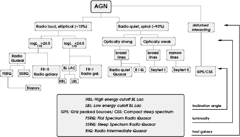
Today, it is known that QSOs fit into the general classification scheme of Active Galactic Nuclei (AGN), objects which are believed to be powered by a rotating supermassive black hole in the center of the galaxy. A schematic view of the general picture of AGN is shown in Fig. 4. The core is “active” due to the accretion disk which forms around the central black hole and radiates strongly at optical frequencies. The disk is fed by matter from a dust torus. Perpendicular to the accretion disk, two relativistic jets are emitted, transporting matter in form of lobes. Knots and hot spots along the jets emit radio emission, leading to the strong observed radio signal of AGN. It is expected that these knots and hot spots represent shock environments in which particles are accelerated to high energies, in the case of hadrons up to proton energies of eV, see BS (87). In this section, a general classification scheme for AGN is presented as well as spectral and temporal properties of the sources.
AGN unification scheme
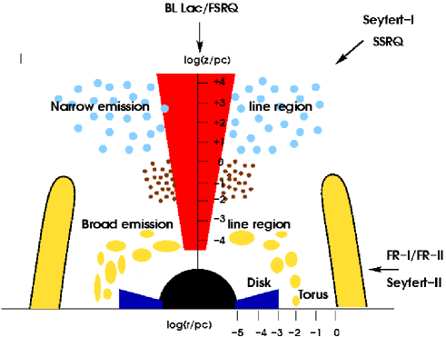
Three main criteria can be used for the unification scheme of Active Galactic Nuclei which is indicated schematically in Fig. 5:
-
1.
The activity of the source at radio wavelengths yields a division into radio loud and radio weak objects. About 90% of all AGN are radio weak and are usually hosted in spiral galaxies, while radio loud nuclei are located in the centers of elliptic galaxies.
-
2.
The luminosity of the object is a further classification criterion. Radio weak sources are subdivided into optically strong and optically weak sources, which can be distinguished by considering the features of the emission lines. Optically strong sources usually lack narrow emission lines which are present in the optically weak case. Both source types appear to have broad emission lines. Radio loud sources with extended jets ( kpc) are subdivided at radio wavelengths into low luminosity and high luminosity objects at a critical luminosity of W/Hz. The jets of compact objects such as GHz-Peaked Sources (GPS) and Compact Steep Sources (CSS) are believed to get stuck in matter.
-
3.
The third classification criterion is the orientation of the AGN towards the observer. AGN are axisymmetric along the jet axis. In the branch of radio loud AGN, an object is classified as a blazar if one of the jets is pointed directly towards the observer. Flat Spectrum Radio Quasars (FSRQ) are the high luminosity population of the blazars while BL Lacs form the corresponding low luminosity population. So called Faranoff Riley (FR) galaxies are being looked at from the side, so that jets and torus are usually clearly visible. The high luminosity FR-II galaxies show a very strong radio emission at the outermost end of the jets, while the radio emission of the low luminosity class FR-I happens in knots throughout the jet.
For radio weak AGN, the objects are called radio weak quasars in the optically strong case and Seyfert-I galaxies in the optically weak case when looked at the gap between jet and AGN torus. The radio weak equivalent to FR galaxies are Radio Intermediate Quasars (RIQ) and Seyfert-II galaxies, where the observer’s view is directed towards the torus.
Multiwavelength observations of AGN
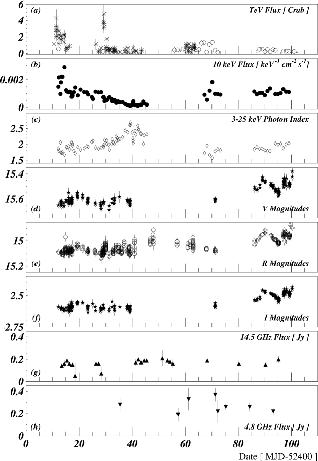
AGN have been observed in all frequency bands, ranging from radio observations up to TeV measurements. As an example, the lightcurves of the BL Lac object 1ES 1959+650 have been investigated in a multiwavelength campaign between May 18, and August 14, 2002 K+ (04). The results are shown in Fig. 6. The bandpasses shown are TeV emission as detected by Whipple (stars) and HEGRA444High Energy Gamma-Ray Astronomy (circles), X-ray emission as measured by RXTE555Rossi X-ray Timing Explorer, optical emission in the Violett, Red and Infrared band as well as radio measurements from UMRAO666University of Michigan Radio Astrophysical Observatory at frequencies of GHz and GHz. As can be seen from the example, AGN are highly variable objects at all wavelengths. In multiwavelength campaigns as the presented one, the correlation between the temporal behavior in the different bandpasses is examined. Such campaigns are relevant to determine the origin of the radiation. In the case of the observation of 1ES 1959+650, a so-called orphan flare was observed, representing a rapid increase in intensity only at TeV energies. Since SSC models necessarily predict the correlated emission of TeV photons and X-rays, this scenario can be excluded for the observed flare, while an EC scenario is still possible. A hadronic scenario in which the TeV photons come from the decay of particles produced in proton-photon interactions does not require the connection between X-rays and high-energy photons. Orphan flares are therefore very interesting in the context of neutrino emission.
Recent results from Aha+06a could restrict the temporal variability at TeV energies to less than days. This implies scales of the order of the Schwarzschild radius of M 87, indicating that the TeV signal originates from the core of the object and not from the jets.
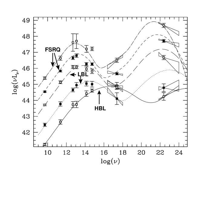
Most recently, the detection of 3C 279 by MAGIC at energies of was announced PM+ (07). The detection this distant source was unexpected, since very high-energy photons are believed to be absorbed by the interaction with the infrared (IR) background, see also Section 3.2.1. The flux at energies of above GeV is therefore expected to be absorbed completely for sources with distances above . The spectral energy distribution (SED) of AGN typically shows two main bumps, see Fig. 7, apart from dust radiation, which can also lead to a bump in the spectrum, see e.g. C+ (89). The lower energy hump is believed to arise from synchrotron radiation of electrons. Different radiation processes can be responsible for the second hump at higher energies (GeV-TeV): in the Synchrotron Self Compton scenario, the synchrotron photons are up-scattered to high energies by the primary electrons by the Inverse Compton effect. This implies the direct correlation of the two humps in the case of an intensity variation. A second possible scenario is the production of TeV photons in -decays. particles are produced in hadronic interactions with photon fields or with each other in the source. Such a hadronic scenario leads to the coincident production of high-energy neutrinos. It does not necessarily imply the coincident variation of the lower and higher energy hump, since the two emission signatures are not directly linked. A third component which can contribute at TeV energies is the synchrotron radiation of protons. The latter radiate in the case of high magnetic fields in the acceleration region. Depending on the energy range of the second hump in the SED, BL Lac objects can be divided into a further sub-class of High-peaked BL Lacs (HBLs), Low-peaked BL Lacs (LBLs) and Flat Spectrum Radio Quasars (FSRQs). If the peak occurs at TeV energies, sources are called HBLs, while they are referred to as LBLs at peak energies in the GeV range. The source is called FSRQ for even lower peak energies. The source classes can be identified by taking their radio emission at GHz as a measure. Figure 7 shows the SED for a sample of blazars presented in F+ (98). The sample is divided into five sub-samples, selected via their radio luminosity at GHz, erg. The overlaid curves are analytic approximations as described in F+ (98).
TeV photons from AGN and the extragalactic background light
Since 2003, the second generation of Imaging Air Cherenkov Telescopes (IACTs) is taking data, with leading results from H.E.S.S.777High Energy Stereoscopic System and MAGIC888Major Atmospheric Gamma Imaging Cherenkov Telescope, and most recently also from VERITAS999Verv Energetic Radiation Imaging Telescope Array System. As of December 2007, 17 HBLs have been detected. Most recently, the first LBL, BL Lacertae, has been identified at TeV energies by the MAGIC experiment AM+07a . In addition, M 87 as a misaligned blazar, or a FR-I galaxy, is identified at energies of GeV. With 3C 279, the first FSRQ has now been identified by MAGIC at GeV. This source is by far the most distant object detected at these high energies. The AGN identified at TeV energies and their spectral properties are listed in table 2. It is not possible to give a time-independent spectral parameterization of these variable TeV sources, since both the spectral index and the normalization vary with the intensity of the signal. In the table, intense flare events have been chosen. The values represent the maximum output per second observed so far. The parameterization for the spectra is taken as
| (23) |
with the spectral parameters as measured at Earth. The signal of TeV photons is (partially) absorbed at the highest energies by the Extragalactic Background Light (EBL), comprised of the infrared background as the trace of star formation, the cosmic microwave background and other photon fields in the Universe SdS (92). For a lower energy threshold of GeV, it was expected that sources up to can be detected. Thus, the detection of 3C 279 at was unexpected and makes it necessary to reconsider the basic physics. Two assumptions go into the conclusion that sources farther away than should be completely absorbed at GeV: (a) the presence of the IR background from star formation; (b) the intrinsic particle spectra are not flatter than . With the detection of 3C 279, it is most likely that one of the assumptions does not hold. The intensity of the EBL at IR wavelengths is difficult to determine directly. However, star formation unavoidably leads to the production of at least a minimum component of IR radiation. The observation of such a distant source is difficult to explain by altering the EBL model within the standard models of cosmology and particle physics. Beyond the standard model of particle physics, it is possible to introduce a new boson as done in AMR (07). Photons are in oscillation with a light boson of a mass eV, leading to the significant reduction of the ELB. An further approach is presented in PM (00), explaining the long attenuation length via the violation of the Lorentz invariance at the highest energies. An explanation within the standard model is that the photon spectra are indeed extremely flat intrinsically, which can be the result of very flat primary particle spectra. The statement from Aha+06b that the photon spectra can intrinsically not become flatter than is questioned in SBS (07). The basic assumption which produces the limit is that the primary particle spectra producing the Inverse Compton component at GeV-TeV photon energies is not flatter than as it was shown by BO (98); K+ (00); OB (02) for relativistic, parallel shocks in the small angle scattering regime. It is pointed out in different papers, however, that the assumed shock configuration is very specific and does not apply to most sources Bar (04); MBQ07a ; MBQ07b . In SBS (07), it is shown that using larger scattering angles, very flat spectra can be produced. This leads in turn to flatter IC spectra, making it possible to extend the absorption cutoff to higher redshifts. To resolve this issue, further observations of more distant object are necessary, and the lowering of the threshold energy for photon detection to a few tens of GeV will also help.
While IACTs are designed for the detection of point sources, surface water Cherenkov detectors instrument a large area with photomultipliers, being able to observe both photons, electrons and muons from electromagnetic showers. This technique allows for the observation of sr at once, however, with a relatively low sensitivity and a high-energy threshold. MILAGRO succeeded with the observation of Mkn 421 and the Crab nebula. In addition, diffuse emission regions in the Cygnus region were found, which is not possible with IACTs due to the small field of view. The next generation water Cherenkov telescopes, including the planned HAWC101010High Altitude Water Cherenkov experiment SSM (05); S+ (06), are expected to give more information on diffuse emission due to a higher sensitivity.
| Source | type | first TeV | |||
| detection | |||||
| /(TeV s cm2) | Ref | ||||
| M 87 | FR-I | 0.004 | HEGRA | ||
| (H.E.S.S. 2005) | Aha+06a | Aha+03a | |||
| Mkn 421 | HBL | 0.031 | Whipple | ||
| (Whipple 2001) | K+ (01) | PW+ (92) | |||
| Mkn 501 | HBL | 0.034 | Whipple | ||
| (HEGRA 1997) | Aha+ (99) | QW+ (96) | |||
| 1ES 2344+514 | HBL | 0.044 | Whipple | ||
| (Whipple 1995) | S+05b | CW+ (98) | |||
| Mkn 180 | HBL | 0.045 | MAGIC | ||
| (MAGIC 2006) | AM+06a | AM+06a | |||
| 1ES 1959+650 | HBL | 0.047 | Tel. Array | ||
| (HEGRA 2002) | Aha+03b | Nis (99) | |||
| BL Lacertae | LBL | 0.069 | MAGIC | ||
| (MAGIC 2006) | AM+07a | AM+07a | |||
| PKS 0548-322 | HBL | 0.069 | n/a | n/a | H.E.S.S. |
| - | - | DH+ (07) | |||
| PKS 2005-489 | HBL | 0.071 | H.E.S.S. | ||
| (H.E.S.S. 03/04) | Aha+05a | Aha+05a | |||
| PKS 2005-489 | HBL | 0.071 | H.E.S.S. | ||
| (H.E.S.S. 03/04) | Aha+05a | Aha+05a | |||
| RGB J0152+017 | HBL | 0.080 | n/a | n/a | H.E.S.S. |
| - | - | NC+ (07) | |||
| H 1426+428 | HBL | 0.129 | Whipple | ||
| (Whipple 2001) | P+ (02) | HV+ (01) | |||
| 1ES 0229+200 | HBL | 0.139 | H.E.S.S. | ||
| (H.E.S.S. 05/06) | Aha+07a | DH+ (07) | |||
| H 2356-309 | HBL | 0.165 | H.E.S.S. | ||
| (H.E.S.S. 2004) | Aha+06c | Aha+06c |
| Source | type | first TeV | |||
| detection | |||||
| /(TeV s cm2) | Ref | ||||
| 1ES 1218+304 | HBL | 0.182 | MAGIC | ||
| (MAGIC 2005) | AM+06b | AM+06b | |||
| 1ES 1101-232 | HBL | 0.186 | H.E.S.S. | ||
| (H.E.S.S. 2006) | Aha+07b | Aha+07b | |||
| 1ES 0347-121 | HBL | 0.188 | H.E.S.S. | ||
| Aha+07c | Aha+07c | ||||
| 1ES 1011+496 | HBL | 0.212 | MAGIC | ||
| (MAGIC 2006) | AM+07b | AM+07b | |||
| 3C 279 | FSRQ | 0.538 | n/a | n/a | MAGIC |
| - | - | PM+ (07) | |||
| PG 1553+113 | HBL | ? | H.E.S.S. | ||
| Aha+06d | |||||
| -4.2 | 2.1 | MAGIC | |||
| (MAGIC 05/06) | AM+07c | AM+07c |
3.2.2 Gamma Ray Bursts
Photon eruptions of unknown origin were detected in the 1960th by both American and Soviet military satellites. While it was immediately clear that these events were not man made, but originated from outer space, the publication of the first observation in 1967 did not happen before 1973 in the case of the Vela Satellites KSO (73) and only a few months later in the case of the Soviet Kosmos-461, and the American OSO-7111111Orbiting Solar Observatory-7 and IMP-6121212Interplanetary Monitoring Platform-6 satellites W+ (73); CD (73); MGI (74). Systematic studies of these Gamma Ray Bursts (GRBs) were done with BATSE131313Burst and Transient Source Experiment on board of the CGRO141414Compton Gamma Ray Observatory which was taking data for 9 years, between April 1991 and June 2000 P+ (99). During that time, 2704 GRBs in the energy range of keV were detected151515In the following, the detection energy range of all quoted instruments is given in the notation for simplicity..
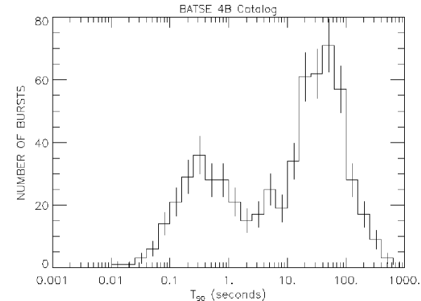
Figure 8 shows the distribution of the duration of the bursts BAT (08); P+ (99), defined in the way that 90% of the signal was received during that time. Two populations of bursts can be identified, classified as “short” ( s) and “long” ( s) bursts. The spatial distribution of GRBs in galactic coordinates as observed by the BATSE reveals an isotropic distribution with no visible clustering in the galactic plane or anywhere else. This indicates an extragalactic origin of the events. However, scenarios of a galactic halo with so far unknown sources of GRBs were also proposed, see e.g. H+ (94); PRR (95); FS (96). A first indication of a cosmological origin was given by the spatially non-Euclidean distribution of the source luminosity. The final proof of the cosmological distance of GRBs was possible in 1997 by the first afterglow observation by the BeppoSax161616Beppo stands for Guiseppe Occhialini, and “SAX” is an acronym for Satellite per Astronomia X satellite, see e.g. WRM (97). While the prompt emission is mainly detected in the keV-MeV band, the so-called afterglow continues until long after the prompt emission and is seen in basically all wavelength-bands, from the radio band up to GeV-energies. From the afterglow-observation, host galaxies can be identified, or absorption and emission lines can be measured to determine the redshift at which the GRB occurred. These redshifts are cosmological, so that GRBs are known to happen outside of our Galaxy. The reason for the intense discussion of a galactic origin was that the photon fluence in the keV energy band as measured by BATSE scatters around
| (24) |
The term ”fluence” is used here as opposed to flux, since the units are erg/cm2, while a flux is typically measured per area and time interval. For extragalactic distances, the total luminosity of a GRB event lies around
| (25) |
for isotropic emission, but a little bit lower in the case of beamed emission favored currently. This tremendous output lies more than four orders of magnitude higher than the typical output of AGN, the most luminous permanent source class in the sky,
| (26) |
While GRBs emit only for a short time of a few seconds, AGN are active over long periods, so that the time integrated output is comparable, erg. In the past decades, different models have been developed to explain the output from GRBs and AGN. Many of the classical arguments for the description of GRB physics are borrowed from supernova remnants Wol (72); Cox (72); CS (74) or AGN models Ree (70), since the phenomena are similar, although on different spacetime-scales. Both AGN and GRBs show a variable time structure. supernova remnants as well as long GRBs are produced in the explosion of stars. In all three objects, shock fronts are responsible for particle acceleration and therefore, the non-thermal electromagnetic spectrum can explained by synchrotron radiation of electrons, Inverse Compton scattering and also by proton-photon interactions. The favored model which is able to explain most of the phenomena connected to a GRB is the fireball model, explaining the huge electromagnetic emission by shock formation of relativistic plasma shells, see e.g. Pir (99, 05); ZM (04). Alternatively, the Cannonball model tries to explain GRBs by colliding plasma balls, see e.g. DR (04); Dar (06). However, the latter meets observations difficult to match the predictions in this model, e.g. the prediction of apparent motion for the radio emission, which is not observed for GRBs. Thus, only the fireball model will be discussed in more detail in the following paragraph.
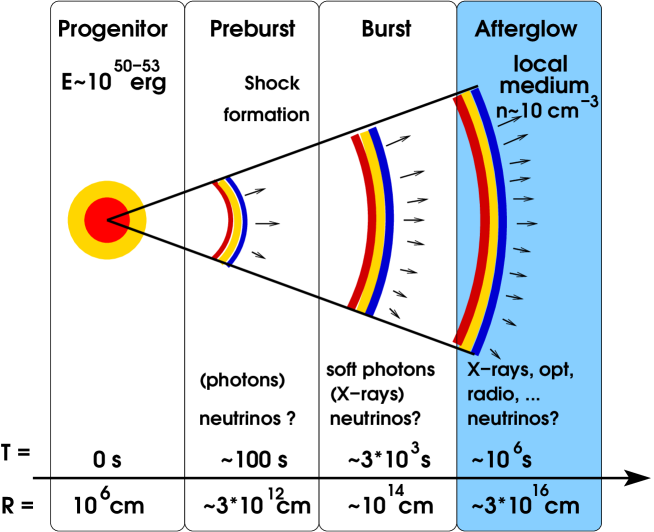
Fireball model
A schematic view of the fireball model is shown in Fig. 9. It is based on the model of stellar outbursts as described in Sed (58) and was enhanced including relativistic effects in order to match GRB observations. The fireball model does not give any constraint on the progenitor. It yields a phenomenological description of the actual burst observations. The basic idea is that a large amount of mass is ejected within a short time interval by a central engine. The plasma is ejected successively in shells. At some point, the outer shells slow down and are caught by inner shells and a shock front is built up, accelerating electrons and baryons in the plasma up to high energies. While protons can be accelerated basically loss-free up to energies as high as eV Vie (95); Wax (00), electrons lose their energy to synchrotron radiation, escaping from the shocks as soon as the region becomes optically thin. This is observed as prompt emission from GRBs. Those shocks resulting from collisions of shells are called internal shocks. So-called external shocks result from collisions of the shells with the interstellar medium leading to afterglow emission as described in the following paragraph. While the prompt emission occurs mainly at energies of keV, afterglow emission is observed in almost all wavelength bands. Reviews on the details of the underlying physics are given in e.g. Pir (99, 05); ZM (04).
GRB experiments after BATSE
After the BATSE era, many GRB satellites were taking data, each covering a much smaller field of view and thus providing much less statistics than BATSE. Additionally, many of the satellites were not able to give directional information. For the determination of the GRB spatial origin, it is necessary to have at least three detectors. BATSE had four energy channels and could localize GRBs. The precision was between approximately and a few degrees. Other satellites have only one or two instruments on board. To improve the localization of GRBs, the Interplanetary Network was created already in the 1970s as an interconnection of all GRB satellites. The currently active third Interplanetary Network, IPN3, was formed with the launch of Ulysses in 1990 H+ (92); Uly (08). Since the beginning, more than 25 spacecraft missions have participated. The CGRO joined in 1991 when it was launched. Today, HETE-II171717High Energy Transient Explorer-II S+05a ; HET (08), INTEGRAL181818INTErnational Gamma-Ray Astrophysics Laboratory Win (04); M+05b , RHESSI191919Ramaty High Energy Solar Spectroscopic Imager RHE (08), Mars Odyssey H+ (06); Mar (08), Ulysses H+ (92); Uly (08), Konus Wind M+05a ; Kon (08) and Swift form the IPN3. The most important GRB experiments with some of their individual properties are listed in table 3. With information of more than two instruments, GRB positions of a accuracies up to several square-arcminutes can be reconstructed. Before the launch of BeppoSax in 1996, this was the only possibility of arcminute precision measurements. HETE-II and INTEGRAL are able to localize GRBs without additional information from IPN3. Konus is very sensitive to short GRBs and a catalog of short GRBs is examined in the context of neutrino emission, see Section 7.
| GRB Sat. | Launch-Demise | FoV∗∗∗ | E-range | Localiz. | Reference |
| [keV] | Precision | ||||
| Vela 5B | 05/1969-06/1979 | (3, 750) | - | KSO (73) | |
| Kosmos-641 | 12/1971-09/1972 | sr | (28, 1000) | - | MGI (74), |
| Pal (07), | |||||
| M+ (75) | |||||
| Ulysses∗ | 10/1990-now | (5, 150) | - | H+ (92), | |
| Uly (08) | |||||
| BATSE | 04/1991-06/2000 | sr | (20, 2000) | degree | P+ (99), |
| BAT (08) | |||||
| BeppoSax | 04/1996-04/2002 | (0.1, 300) | arcmin | B+ (97), | |
| Bep (08) | |||||
| Mars Od.∗ | 04/2001-now | (50, 10000) | - | H+ (06), | |
| Mar (08) | |||||
| NEAR | 02/1996-02/2001 | (1, 10000) | - | NEA (08) | |
| Konus W.∗ | 11/1994-now | sr | (10, 10000) | - | Kon (08) |
| RHESSI∗ | 02/2002-now | (3, 20000) | - | RHE (08) | |
| INTEGRAL∗ | 10/2002-now | M+05b | |||
| SPI | (18,8000) | - | |||
| IBIS | (15, 10000) | arcmin | |||
| HETE-II∗ | 10/2000-now | sr | (0.5, 400) | arcmin | HET (08), |
| S+05a | |||||
| Swift∗ | 11/2004-now | Chi (06), | |||
| BAT | sr | (15, 150) | arcmin | Swi (08) | |
| UVOT∗∗ | (170, 650) | arcsec | |||
| XRT | (0.2, 10) | arcsec |
The Swift satellite was launched in November 2004 - for a review seee.g. Chi (06) and references therein. Swift is a dedicated GRB satellite with four instruments on board. The main purpose of the BAT202020Burst Alert Telescope detector is the discovery of prompt emission from GRBs. The main sensitivity is in the energy range of keV and the field of view is about sr. About 100 GRBs per year are detected with BAT. The XRT212121X-Ray Telescope covers an energy range of keV and serves afterglow observations. The UVOT222222UV/Optical Telescope is an instrument for the detection of the optical afterglow at nm wavelengths.
The advantage of a satellite carrying both prompt emission and afterglow instruments is that the afterglow can be followed almost starting from the prompt emission phase. This has already lead to the discovery of unexpected temporal behavior directly after the prompt emission, see e.g. Més (06) for a review. The basic features of the early afterglow are shown in Fig. 10. While the afterglow appearance at s after the prompt emission had been known before, the temporal behavior at earlier times was unexplored until the launch of Swift. Two main features are found. Firstly, a break in the temporal decay structure is observed. The decay index changes from to at around s to s after the prompt emission and it changes back to the previously observed behavior at s to s. Secondly, X-ray flares are detected during the early afterglow, indicated by the dashed triangle in the curve. X-ray flares occur only in a fraction of the observed bursts. Different models to explain both the changes in the decay index and the X-ray flares have been developed which are reviewed in e. g. Més (06).

Observed Redshifts from GRBs and GRB progenitors

The first afterglow observation by BeppoSax for GRB970228 also implied the first measurement of the redshift of a GRB. Between 1997 and November 2004 - the time of the launch of Swift - redshifts of 44 GRBs have been detected. Since the launch of Swift, 58 long and 6 short GRB redshifts were measured as of March 12 2007. Figure 11 shows the redshift distribution of those GRBs. The solid line represents Swift bursts while the dashed line shows pre-Swift measurements of redshifts. The mean of the distributions is shifted, Swift observations show a higher contribution of very distant bursts. One reason for this is the better sensitivity of Swift compared to pre-Swift instruments. Bursts at high redshifts have typically a weaker fluence and may have been missed by instruments of lower sensitivity. The higher statistics of bursts with measured redshifts relies on the possibility of early afterglow observation of the Swift instruments XRT and UVOT.
It is known since 2003 that long GRBs are connected to supernova explosions of type Ic, which follow the death of Wolf-Rayet stars M+03a . Two scenarios of producing jets in exploding stars have been discussed:
- 1.
- 2.
Short bursts have been proven in 2005 to originate from the merging of two neutron stars or a neutron star and a black hole in a binary system H+ (05); V+05c ; G+06b . The differences in the observed events lie not only in the duration of the bursts, but are also seen in the redshift distribution. While long GRBs are most likely to follow the star formation rate and are located in starforming regions, short bursts happen in regions of rather low star formation rate and at small redshifts .
New results from the Swift satellite show, however, that this scheme is still too simple: there are exceptional bursts which do not fit into this scheme (e.g. GRB060218, GRB060614) C+06a ; G+06a . Also, Swift does not see the strong distinction between short hard and long soft bursts as it was observed by BATSE SaS (06). This indicates that the classification scheme is more complex than it can be determined yet and needs to be refined in the future.
Classification of GRBs
In order to explain the observation of the prompt emission in GRBs, a boost factor of for the shock fronts is necessary. For lower boost factors, the shock region is optically thick to pair production processes. On the other hand, the boost factor must not exceed , since protons would lose most of their energy due to synchrotron radiation in that case HaH (02). The peak energy of the GRB, is directly correlated to the boost factor and lies around keV for regular GRBs. Typically, a boost factor of is assumed. The two main sub-classes of GRBs are long and short ones. The differences do not only lie in the duration of the events, but also in the hardness of the spectra. Short bursts typically have much harder spectra than long GRBs which is why they are usually referred to as Short Hard Bursts (SHBs).
A measure for the hardness is the ratio of soft to hard emission,
| (27) |
with as the photon flux. In the case of BATSE, which had four energy channels, channel 3 with an energy range of keV and channel 4, keV were used to determine the hardness ratio. Bursts with s are generally harder than long bursts ( s). It should be noted, though, that follow-up experiments like HETE-II, Konus and Swift do not see equally hard short bursts. For more details, see SaS (06).
Detailed studies by HETE-II have shown that apart from the regular, long GRBs, there are bursts having peak energies in the X-ray regime S+05a . For the classification of events in terms of the energy band of emission, the hardness ratio for the flux at keV and keV was examined:
| (28) |
Regular GRBs have . About 2/3 of the 45 HETE-II bursts have, however, . This class of GRBs peaking in the X-ray regime, has further been subdivided into X-Ray Rich bursts (XRRs) with X-ray and soft -ray emission, , and X-Ray Flashes (XRFs) with only X-ray emission, . The ratio between these three burst classes as observed by HETE-II is
| (29) |
A schematic view of the classification of GRBs into long and short events and the further subdivision of the long events into regular GRBs, XRRs and XRFs is shown in Fig. 12. The ratio of long to short GRBs is indicated of as detected by BATSE P+ (99). However, HETE-II rather detects a ratioof . The detection ratio should be considered as dependent on the instrument properties232323Swift for instance detects only one short GRB for 18 long ones. This is also due to the fact that Swift detects at relatively low energies keV, while the emission for short GRB rather happens at higher energies as discussed before.. For the analysis of the GRB-XRR-XRF relation, however, it is stated that not many GRBs are missed relative to XRR and XRF events due to any observational effects S+05a , so that a 1:1:1 ratio seems to be reasonable.
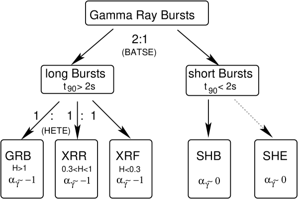
One interpretation of the strong variation of the peak energy is based on variations in the baryonic load of the shocks, which is an important parameter for the development of the boost factor DCB (99). With a high baryonic load in the evolving jet, the system cannot be accelerated to high energies due to the high mass of the baryons. Thus, a this dirty fireball has boost factors of an order of magnitude less than a regular GRB, . Since the peak energy evolves with , the typical values for dirty fireballs are keV and XRRs or XRFs are observed. GRBs as typically observed by BATSE are classified as regular fireballs. Clean fireballs have a very low baryonic load and thus, a high gamma of around , leading to peak energies of MeV. The duration of such short high-energy bursts (SHE) would be small, since the lack of heavy baryons enables the jet to evolve more rapidly, so that s. Such events have, however, not been observed yet. With the launch of GLAST242424Gamma-Ray Large Area Space Telescope, the detection of such phenomena will be possible GM (99). A summary of the different burst types and their basic parameters is given in table 4. The fact that most bursts occur as regular fireballs shows that a certain fraction of baryons needs to be present in the jet which inevitably leads to the production of neutrinos in proton-photon interactions. The question about the intensity of such a neutrino signal has still to be solved.
| parameter | clean | dirty | regular |
|---|---|---|---|
| (XRR/XRF) | (GRB) | ||
| [keV] | |||
| [s] | 0.1 |
The classification scheme as presented here needs to be refined including a more detailed view on the matter in the future: today, there are several bursts which fall out of the scheme, e.g. GRB060218 and GRB060614, and Swift seems to detect a different sub-class of short bursts as compared to BATSE SaS (06). A summary of the observation of the different sub-classes (XRF/GRB/short) with Swift is given in Z+ (07). In Z+ (07), the detection of the shallow decay of the early afterglow as recently observed in many Swift bursts as energy injection features. Such a scenario disfavors the interpretation of XRFs as low GRBs. Swift will help to improve the current classification scheme. For now, the scheme as presented above is still useful, since it can describe the majority of bursts.
3.2.3 Galactic sources
The electromagnetic output of galactic sources of non-thermal emission can be used to estimate their contribution to the Cosmic Ray spectrum.
The Cosmic Ray luminosity can be written as
| (30) |
assuming the production of Cosmic Rays in the Milky Way with a residence time yr in the volume of the galactic disk cm3. Here,
| (31) |
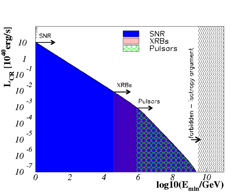
is the Cosmic Ray energy flux. The Cosmic Ray luminosity depends on the minimum energy which is produced. The calculation can only be valid at energies below the ankle, eV: at the highest energies( eV), the observed spectrum is too isotropic to be of galactic origin. Figure 13 shows the Cosmic Ray luminosity versus minimum energy. Three potential source classes are indicated as filled/hatched areas below the curve. In the following, the different source classes will be reviewed with their potential contribution to the Cosmic Ray luminosity. Here, it is assumed that the luminosity in Cosmic Rays produced by a source class must be less than the total electromagnetic output of the same class, .
Supernova remnants
The CR spectrum at energies below the knee is commonly believed to be produced by the shock fronts in expanding shells of supernova remnants (blue filled area). When a star perishes in a supernova (SN) explosion, the emitted material encounters the interstellar medium (ISM), building a shock front of typical velocities m/s. With the typical rate of SN explosions in a galaxy, , and a mean ejected mass of per SN, the supernova remnant’s shock front is active for about yr. The luminosity of a single SNR, erg/s, can then be converted into the total luminosity of SNRs in the Milky Way,
| (32) |
Given the integral luminosity required for the production of Cosmic Rays at eV,
| (33) |
SNRs are good candidates for the production of Cosmic Rays. It is, however, difficult to explain the break in the spectrum at eV. One possibility is that leakage of particles out of the Milky Way becomes important, leaving only heavy elements at the higher energies. This can lead to a steepening of the spectrum. Another possibility is that SN explosions into their own winds can be able to accelerate particles to higher energies, since higher mass numbers (Helium up to iron) are produced. SN explosions of type Ib and Ic lose their hydrogen (for Ic also the helium) envelope before collapsing. This leads to a higher density of particles when the shock forms and thus to different shock conditions. Regular SNRs can in this scenario produce CRs up to the knee and SNR-Winds are responsible for the spectrum between the knee and the ankle.
Pulsars, X-ray binaries and microquasars
As an alternative explanation for the contribution above the knee, systems including neutron stars or black holes are considered.
Neutron stars can be observed due to their emission of electromagnetic radiation along the magnetic field axis. Since the rotational axis of the objects does not align with the magnetic field axis, they are observed as pulsars: the emission is only seen when the particle jet points towards Earth. Pulsars have periodic signals ranging from several seconds down to milliseconds. The Crab as the most prominent, since most luminous, example is a millisecond pulsar. It is a neutron star which was presumably produced in a SN explosion observed on July 04, 1054 252525For a summary of historical SNe including SN 1054, see GS (03).. The pulsar wind nebula has been observed at all wavelengths. From radio up to X-ray energies, the supernova remnant is seen, while the pulsar itself is visible at X-ray and higher energies. The observed TeV signal from the Crab is non-thermal, an indication for particle acceleration in a shock environment, see e.g. Aha+06e . The main reason why pulsars are good candidates for particle acceleration are the very high magnetic fields of around G. Pulsars have spin-down luminosities around erg/s and can therefore not be responsible for the CR flux below the knee. They can, however, contribute to the region between knee and ankle (see Fig. 13, green hatched area, circles).
Magnetars, which are observed as Anomalous X-ray Pulsars (AXPs) or Soft Gamma Repeaters (SGRs), represent pulsars with even higher magnetic fields of G. For a summary on AXPs and SGRs see e.g. WT (04). Five SGR candidates have been observed in the Milky Way so far. These reveal themselves by randomly emitting radiation from time to time. The smaller eruptions have usually thermal spectra, while giant bursts of non-thermal emission are observed from time to time. Famous events are the outbursts of SGR 1806-20 on January 7, 1979 and on December 27, 2004 as well as the giant emission of SGR 1900+14 on August 27, 1998. Flare luminosities of SGRs range from erg/s up to erg/s. AXPs show similar phenomena, but with emission at X-ray energies rather than rays. The original definition of AXPs was the steady emission of X-rays. About half of the AXPs today are known to be variable in X-rays, though. Eight AXP candidates have been observed in the Milky Way so far. The eruptions from magnetars are believed to come from star quakes, exciting the surface of the magnetar which leads to the emission of high-energy radiation. The energy output from AXPs lies at around erg/s.
Binary systems including a neutron star or a black hole are good candidates for shock acceleration as well. X-ray binaries consist of a compact object and companion star. In the case of Low-Mass X-ray Binaries (LMXBs), the non-degenerate star has about a few solar masses. High Mass X-ray binaries (HMXBs) are fed by a blue star (O/B star). Once the companion exceeds the Roche volume of the binary system, it starts to feed the compact object with matter. For HMXBs, accretion can also occur through accretion from stellar winds. The neutron star or black hole in turn emits the gained energy in form of X-rays and sometimes in a jet along the magnetic axis. Such systems can lead to particle acceleration up to the ankle at most. The typical electromagnetic energy of such X-ray binary systems is erg/s. This is much lower than the total energy required to explain the CR luminosity for eV. But considering only events at higher energies, i.e. eV leads to a much lower CR luminosity due to the steeply falling spectrum (see Fig. 13, red hatched area, lines). For a summary of the XRB and CR connection, see e.g. Gai (90).
A special case of an X-ray binary is the so-called microquasar, which are X-ray binary systems with photon emission along two co-linear jets. Such a phenomenon has for instance been observed in GRS 1915+105 MR (94). It is believed to be caused by instabilities in the accretion disk of the system. A burst is caused every time a particularly large amount of matter is accreted from the accompanying star. The development of the burst can be traced by the observation of the electromagnetic emission. Enhanced X-ray emission is seen close to the accretion disk, and radio to optical emission can be observed along the jet. For a recent summary of microquasar physics, see Mir06a .
For binary pulsar systems, a heavy Be-star or O star is accompanied by a neutron star. Periodic emission of high-energy photons can be observed in this case: Be-stars are massive stars with a circumstellar disk. The path of the neutron star around the Be-star is highly elliptic. This can lead to the accretion of matter by the neutron star from the massive star only near the periastron, the point of closest distance of the two stars as discussed in Mir06b . A periodic emission of TeV photons was observed from three systems in the Milky Way, LS 5039 and PSR B1259-63 were detected by the H.E.S.S. experiment Aha+06f ; Aha+05b , while LS I 61+303 was seen by MAGIC AM+06c .
3.3 High-energy neutrinos from astrophysical sources
Neutrinos are produced in astrophysical shock fronts in proton-photon and/or proton-proton interactions via pion-production. The dominant channels are
| (36) | |||||
| (39) |
The same processes occur for incident neutrons instead of protons, leading to the production of particles. At higher energies, kaons can also contribute to the spectrum Rac (00). Higher order processes are usually referred to as multipion production processes. The total cross section for proton photon interactions in the center of mass system is shown in Fig. 14.

While the resulting neutrons are likely to interact before decaying, charged pions decay and produce neutrinos,
| (40) | |||||
| (41) |
3.3.1 Neutrino oscillations
Assuming that pions of negative and positive charge occur equally, the production flavor ratio of neutrinos at the source is
| (42) |
This implies that tau neutrinos are not produced in astrophysical sources. However, since neutrinos have non-vanishing mass eigenvalues, they oscillate on their way to Earth. Neutrino flavor-eigenstates , , are connected to neutrino mass-eigenstates , via
| (43) |
Here, is the eigenvalue for the Hamiltonian operator in vacuum, and thus the energy of the mass-eigenstate. The mixing matrix depends on three angles, and , and a phase . The matrix is given as
| (44) |
Here, and , and . The probability for a neutrino to oscillate from a flavor state to a flavor state in a time starting from the emission of the neutrino at the source, , is given as
| (45) | |||||
| (46) |
for units of . Here, is the difference of the squared masses of two flavors and . While solar neutrino detection basically provides measurements for , i.e. the oscillation from electron neutrinos to muon neutrinos, atmospheric neutrinos provide , where muon neutrinos oscillate into tau neutrinos. The third angle appears to be the smallest and limits are provided by reactor experiments. The parameter set is approximately given as AS+ (04); AK+ (04)
| (47) | |||||
| (48) | |||||
| (49) |
Thus, the mixing matrix can be written as
| (50) |
For a non-monochromatic neutrino beam, the probability has to be averaged over the energy spectrum. Therefore, the term in the oscillation probability is averaged to for large distances LP (95). Therefore, the oscillation probability is independent of time for distances larger than the size of the solar system. The probability matrix for a neutrino flavor vector of changing to a flavor vector is given as
| (51) |
At the source, the flavor ratio is
| (52) |
Applying Equ. (51), the flavor vector approaches
| (53) |
for path lengths exceeding the size of the solar system.
Thus, equal numbers of electron, muon and tau neutrinos are expected to be observed at Earth.
3.3.2 Normalization of the spectrum
Given that the existence of high-energetic protons in astrophysical environments is bound to neutrino production, the observed flux of charged Cosmic Rays can be used to estimate the neutrino intensity expected from the sources of Cosmic Rays, see e.g. Hal (06) and references therein. The Cosmic Ray energy density above the ankle eV, is expected to be proportional to the neutrino energy density,
| (54) |
The constant of proportionality depends on the optical thickness of the source to proton-photon interactions and on the fraction of energy transferred to the charged pion. The fraction of energy going into the neutron does not contribute to neutrino production. The average energy which is transfered from the proton to the neutrino derives from the fraction of energy going into the charged pion, . The four leptons resulting from the pion decay are assumed to carry an equal amount of energy. Consequently, each neutrino which is produced carries 1/4 of the pion’s original energy. The relation between neutrino and proton energy is therefore .
Due to the second channel in which particles are produced, the neutrino flux is expected to be accompanied by a high-energy photon flux:
| (55) |
The resulting photons are produced at TeV energies. Thus, optically thin sources emit TeV photons in coincidence with high-energy neutrinos and the energy densities are proportional:
| (56) |
The constant of proportionality depends on the fraction of energy going into pion production. For optically thin sources, in the case of interactions, of the proton energy goes into each pion flavor and the energy in corresponds to the energy in photons, . For interactions, . If the source of neutrino emission is optically thick to TeV photons, the TeV signal avalanches to lower energies until it reaches a level at which it can escape the source. Thus, sources of GeV to sub-MeV emission can be sources of neutrino production as well, assuming an optically thick environment. Equation (56) holds with different values for and modified integration limits.
In conclusion, the same sources which have been described as the potential origin of Cosmic Rays and which show signs of non-thermal photon emission are selected when discussing neutrino emission. In the following sections, the possibility of neutrino emission from galactic sources like supernova remnants, pulsars and X-ray binaries will be mentioned, as well as the predictions of neutrino production in the decay or interaction of exotic particles like WIMPs or monopoles. Furthermore, extragalactic neutrino emission, i.e. neutrinos from AGN, starbursts and GRBs is discussed.
4 High-energy neutrino detection methods
When a neutrino interacts with a nucleon via charged current interactions, a lepton is produced,
| (57) |
Here, indicates the hadronic product of the interaction, leading to a hadronic cascade. Charged particles in a medium emit Cherenkov light if traveling faster than the speed of light in the same medium. The Cherenkov effect is described in detail in Jac (06). The blue Cherenkov light can be detected by photomultiplier tubes and both the incidental direction and the neutrino energy are reconstructible. The signatures for electrons, muons and tauons are very different. Electrons and tauons produce electromagnetic and hadronic cascades within the detector. About 20% of the total energy go into the hadronic cascade, which arises from the nuclear recoil. The remaining 80% of the energy are carried by the electromagnetic cascade, produced by the charged lepton interacting with the electrons of the medium Kle (04). In contrast, muons only undergo radiation losses and leave track-like signatures. The track of the muon can be reconstructed, since the Cherenkov signal is emitted in form of a directed cone. Tauons have very distinct signatures. A first cascade is produced in the first interaction, where a and a hadronic cascade is produced. The in turn decays, producing a second cascade in which a further is generated. Thus, tau neutrinos have the unique property of regenerating themselves.
In the case of neutral current interactions,
| (58) |
and a hadronic cascade can be observed.
4.1 Signatures
The primary detection technique for Cherenkov arrays is the measurement of neutrino-induced muon tracks in water or ice. To guarantee that the observed muons are neutrino-induced, the Earth is used as a filter. While muons produced in the atmosphere are absorbed by the Earth, neutrinos traverse the Earth and the signature is unique. After the filtering of atmospheric muons, the remaining signal mainly consists of neutrinos produced in hadronic showers in the atmosphere. Various analysis methods have been developed to separate this background from a potential signal from extraterrestrial sources. In addition to the neutrino-induced lepton, a cascade produced at the interaction vertex contributes to the signal.
While the muon leaves an optical track, the cascade events produce a radio and an acoustic signal in addition to the optical emission. The Landau-Pomeranchuk-Migdal (LPM) effect becomes important at the highest energies, eV, where the cross sections for electron bremsstrahung and photon electron-positron pair production are reduced. As deduced in Kle (04), the electromagnetic shower lengthens to about m at eV. Most of the signal is radiated at the end of the cascade for each of the three detection methods - optical, radio and acoustic. This is why a two-component signal can be expected at the highest energies.
In the case of tau neutrinos, instead of a single cascade, multiple cascades are produced due to the regeneration of the tau. With IceCube, so-called double-bang signatures are expected, where two cascades are observed within the instrumented volume. If one of the cascades happens outside the instrumented volume, the signature is called lollipop. A single cascade is observed together with a muon bundle, so that the cascade finally looks like a lollipop. The lower energy detection threshold is given by the fact that the cascade-like events need to be larger than the spacing of the IceCube strings, which is about m. The assumption that the extension of the cascade event needs to be larger than about m leads to a lower detection threshold of PeV, see B+ (03).
The reproduction of tauons renders possible the signal propagation through the Earth. Therefore, tau neutrino cascades are suitable for the investigation of horizontal or Earth skimming neutrino air showers. The cascades are reproduced within the Earth until the shower comes out of the Earth and can be detected by either an Imaging Air Cherenkov Telescope or an air-shower surface array. Regular hadronic or electromagnetic air showers do not traverse the high column density and the neutrino signature is unique. This technique is for instance used by the Auger experiment AA+07b in the case of surface arrays and by the MAGIC experiment in the case of IACTs BM+07a .
4.2 Atmospheric neutrino background
The main background in the search for extraterrestrial neutrinos are atmospheric muons and neutrinos. When primary CRs interact in the upper atmosphere, a shower develops. If the primary is a hadron, e.g. a proton, secondary mesons and muons are produced while the shower propagates through the atmosphere. Secondary mesons like charged pions and kaons produce neutrinos when decaying. The neutrino spectrum is close to an behavior in the energy range of GeV. This is about one power steeper than the primary spectrum, , since a considerable fraction of pions and kaons ( s) interact again before decaying. Neutrinos from pion and kaon decays are usually referred to as conventional atmospheric neutrinos as opposed to prompt atmospheric neutrinos from heavier hadrons.
4.2.1 Conventional atmospheric neutrinos
An analytic description of the muon neutrino spectrum at GeV is given in Vol (80) as
| (59) |
and the electron neutrino spectrum is given as
| (60) |
Here, , and are angle distribution parameters, depending on the zenith angle . The factor is energy dependent as
| (61) |
The values of , , , and are listed in table 5. At lower energies, GeV, the description is given numerically by H+ (95).
| 1 | 0.6 | 0.4 | 0.3 | 0.2 | 0.1 | 0.05 | 0 | |
|---|---|---|---|---|---|---|---|---|
| [GeV] | 121 | 202 | 298 | 392 | 572 | 886 | 1060 | 1190 |
| [GeV] | 897 | 1500 | 2190 | 2900 | 4220 | 6540 | 7820 | 8760 |
| [GeV] | ||||||||
The ratio of neutrinos to anti-neutrinos is energy dependent. In Wei (93) it is given as
| (62) |
The spectrum is one power steeper than the spectral behavior of the primaries, since the probability that pions and kaons interact before decaying increases with the energy Gai (90). The intensity of the spectrum increases with the angle of the neutrino towards the zenith angle. The larger the angle, the lower the density gradient of the atmosphere and therefore, more pion decays are possible for horizontal events as opposed to vertical events.
4.2.2 Prompt atmospheric neutrinos
When heavy hadrons with charm and beauty content are produced in the atmosphere, the resulting neutrino spectrum appears flatter than the one of conventional atmospheric neutrinos. Due to short lifetimes ( s) these hadrons do not interact before decaying for energies up to GeV. Therefore, the spectrum of the prompt neutrinos follows the primary index, . The exact normalization and spectral behavior is difficult to predict. In order to estimate the energy spectrum of neutrinos from hadrons with charm contents, it is necessary to simulate interaction conditions at extremely high energies ( GeV). Interaction models are based on accelerator data reaching particle energies up to GeV at most. The second challenge is the behavior of interactions at small Björken. The Björken scale invariant is given as
| (63) |
Here, is the negative four-momentum transfer, is the nucleon mass of the interaction and is the energy transfer in the laboratory system, see e.g. Sch (97); HM (84). The scale invariant is physically constrained to . Interactions with small values of imply forward-scattered processes. Accelerator experiments only yields measurements for , since the beam pipe does not allow the detection of particles at smaller . Therefore, extrapolations to high energies and small are needed in order to calculate the atmospheric charm flux. Figure 15 shows the atmospheric prediction including conventional neutrinos according to H+ (04) together with different predictions of the prompt atmospheric neutrino flux. At energies of around GeV, the prompt neutrino flux becomes stronger than the signal from the conventional neutrinos. The uncertainties in the models are larger than one order of magnitude. Large volume neutrino detectors can help to determine the flux of prompt atmospheric neutrinos and thereby improve the knowledge of particle interactions at the highest energies.
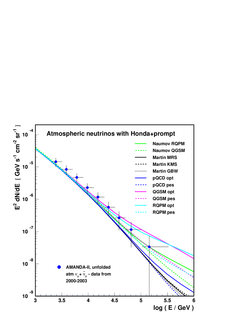
4.3 General detection method
An estimate of the detection rate of neutrino-induced muons/cascades can be given by folding the expected neutrino flux at Earth with the probability of the detection of the neutrino,
| (64) |
Here, is the probability that a neutrino interacts with a nucleus to produce either a muon - - or an electromagnetic or hadronic cascade - cascade - which is detectable in a large volume neutrino detector. It can be written as
| (65) |
where is Avogadro’s constant. The range of the produced lepton within detection range is determined by the geometric detection volume. For the case of muon neutrinos, the resulting muon can be observed even if produced outside the detector itself. The average muon energy loss rate in a medium is given as GHS (95)
| (66) |
The first term occurs due to ionization losses of the muon. Monte Carlo simulations show that can approximately be regarded as a constant with a value of in media like rock. The second term is due to bremsstrahlung, pair production and nuclear interactions. The parameter is determined via Monte Carlo methods, with a value which is approximately constant in a given medium. For rock-like media, . For a discussion of and in the context of muon tracking in a medium using Monte Carlo methods, see RC (01).
The muon range is then given by the integral of the inverse of muon loss rate over the muon energy:
| (67) | |||||
| (68) |
The differential cross section includes charged and neutral current interactions for cascade events, . In the case of a muon signal, only the charged current cross section contributes, . The energy threshold of the detector is given as . The cross section is determined by using the parton distribution functions given by CER . For the calculations in this review, the model of GRV (92) is chosen.
The probability that a neutrino is absorbed by the Earth due to neutrino-nucleon charged and neutral current interactions is given by the shadow factor,
| (69) |
in which is the column depth in units of cmwe and is the mean path that the particle can survive without interacting. The mean free path can be written in terms of the total cross section as follows
| (70) |
Subsequently, the shadow factor can be expressed as
| (71) |
The column depth depends on the traveling distance through Earth. It is also dependent on the Earth’s density layers it has to pass.
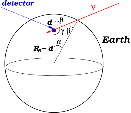
In order to calculate the absorption probability the neutrino’s path through the detector needs to be calculated. Assuming a neutrino is entering the detector under a zenith angle (see figure 16) and applying the sine theorem to the triangle including , and , the relation
| (72) |
is found. is the radius of the Earth while is the depth at which the detector is located under the Earth’s surface. The angle is determined as . Applying the sine theorem once more and using the equation (72) with the approximation , the distance which the neutrino has to travel through Earth is given as262626Note that this is only the case for . For and , the traveling distance of the neutrino through Earth is equal to the depth of the detector under the Earth’s surface : . If, on the other hand, and , the traveling distance is since the neutrino arrives from the opposite direction.
| (73) |
The column depth is the product of the density of the Earth, , with the traveling distance of the neutrino through Earth:
| (74) |
Depending on the zenith angle, the neutrino has to travel through different Earth layers which have different densities. A model of the density profile of the Earth is given in DA (81),
| (75) |
Here, is given as with km as the radius of the Earth.
The energy dependence of the shadow factor and interaction probability is shown in Fig. 17 for the case of electron neutrinos. Solid lines represent neutrinos and dashed lines show anti-neutrinos. The shadow factor is close to unity for low energies, while the interaction probability increases with energy. The product of both determines folded with the neutrino spectrum gives the event rate for a given flux.
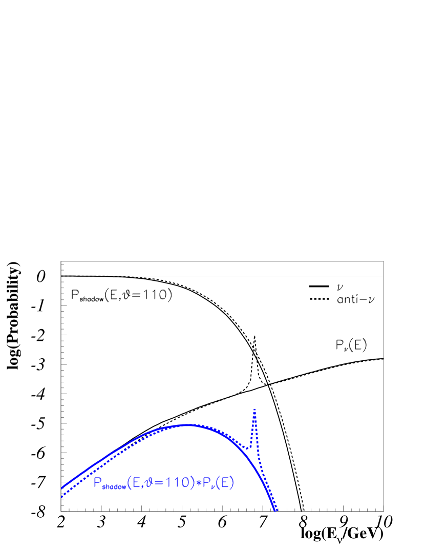
Three main signatures can be detected from neutrino-nucleon interactions. The main detection method is the optical detection of the Cherenkov light. Detectors in water and ice have been and are being built. The main differences between the detector performance in ice and water lie in the scattering and absorption lengths in water and ice. Ice absorbs only little of the light, water has better scattering properties. In water, there are two additional background components, bioluminescence from bacteria populations in the sea water, and light from 40K decay.
Neutrino-induced cascades can also be detected at radio wavelengths and as acoustic pulses. These cascades are detectable over long distances and therefore, radio and acoustic arrays do not need to be instrumented as densely as optical detectors. On the other hand, larger volumes need to be deployed, since the radio and acoustic detection methods become effective at high threshold energies, GeV, at which the expected neutrino flux is already very low.
4.4 Optical detection in ice and water
4.4.1 Ice
The largest currently operating, completed high-energy neutrino detector is AMANDA-II272727Antarctic Muon And Neutrino Detector Array-II. The low neutrino-nucleon cross section demands the instrumentation of large volumes to achieve a significant rate of events. AMANDA is located in the Antarctic ice, between 1500 m and 2000 m below the surface and covers a geometric volume of 0.016 km3. The detector consists of 19 strings with a total of 677 PhotoMultiplier Tubes (PMTs). AMANDA can detect neutrinos with energies of a lower threshold energy of GeV.
AMANDA’s successor IceCube is currently being built around theAMANDA experiment in 1500 m to 2500 m depth. The final configuration will include a geometric volume of km3 with strings, carrying 60 PMTs each. During the past four polar seasons (each year between October and February the following year), a total of 40 strings has already been deployed (1 string in 04/05, 8 strings in 05/06 and 13 strings in 06/07, 18 strings in 07/08).As half a cubic-kilometer is already instrumented, completion of the full cubic-kilometer is expected in 2011. Since the spacing between the PMTs and also between the strings is larger than in AMANDA, the threshold energy is slightly higher, GeV. With the increased volume, higher energy events are easier to identify (the light deposition and the path lengths are increased with increasing energy) and better sensitivities can be achieved.
4.4.2 Water
The optical detection of neutrinos in water via the Cherenkov effect has already been probed by lower energy detectors like (Super)Kamiokande and SNO as discussed above. In the case of high-energy neutrinos, natural water reservoirs are used for detection. The first generation array Baikal detects neutrino-induced cascades and also muons in Lake Baikal AB+06a ; Wis (06). The advantage of this lake is that it is deep enough to deploy m long strings in depths of m and that the detector can be reached in winter due to the thick ice layer covering the lake. Baikal has been taking data with the NT200 detector since 1998. In April 2005, the detector was enlarged to NT200+, enclosing km3 of water. The sensitivity to a diffuse flux for all three neutrino flavors lies around AB+06b .
Currently, different experiments are under construction in the Mediterranean sea. In the ANTARES282828Astronomy with a Neutrino Telescope and Abyss environmental RESearch AA+ (97); Mon (03) project, m long strings are being deployed up to a depth of m AA+ (97); ANT (08). As of December 2007, 10 lines were deployed and the first muon tracks could already be identified. The final detector configuration will consist of 12 strings with an instrumented volume of km3. A second array is being constructed near the coast of Italy, the NEMO292929NEutrino Mediterranean Observatory detector Sap (06); NEM (08), at a depth of m. Such a high depth has two main advantages: the flux of atmospheric muons from above is lower in the detector, and also the bioluminescence background is low at high depths. The first tower was deployed in 2006. In a second phase, the deployment of one or more additional towers are planned. NESTOR303030Neutrino Extended Submarine Telescope with Oceanographic Research is a third experiment, being deployed near the coast of Greece at a depth of m AN+ (05); NES (08). The first phase of the detector was deployed in March 2003, and first results are presented in form of the measurement of horizontal atmospheric muons AN+ (05).
The primary aim of the three arrays described above is to explore different sites and techniques for neutrino detection in sea water in order to build a km3 detector, choosing the optimal location and design, namely KM3NeT KM (308). This detector will be complementary to IceCube, detecting mainly muon neutrinos from the southern hemisphere. With both arrays, a view of the complete sky is possible. The view on the southern hemisphere enables KM3NeT the observation of the galactic center, which is only restrictedly visible from the South Pole.
4.4.3 Analysis strategies
In order to keep the analysis blinded to avoid experimenters bias, analysis cuts are optimized using off-source samples created by scrambling the right ascension of events or excluding the time window of transient emissions under investigation. Diffuse flux analyses are optimized on a low energy sample, where the signal is expected to be negligible.
The search for steady point sources is possible in two ways: the selection of data according to specific source candidates and the search for spatial clustering in the data independent of any source location. The mean sensitivity in the northern hemisphere to an neutrino flux from a point source, , given by the AMANDA experiment is AI+07b
| (76) |
for 5 years of data taking AI+07b .
The search for single point sources can be complemented by stacking classes of sources according to the direct correlation between the photon output and the potential neutrino signal. This was done with AMANDA data for 11 different AGN samples that were selected at different wavelength bands, see AI+06b . The optimum sensitivity was typically achieved by the stacking of the strongest sources in the catalog. The principle of source stacking is indicated schematically in Fig. 18. As an example, three source classes, FR-I and FR-II galaxies as well as blazars, are displayed. The stacking limits are obtained by stacking the most luminous sources of the same class in the sky, indicated by sources with filled circles. Weaker sources (empty circles) are not included.
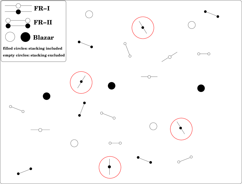
The search for GRBs is almost background free, since the events are selected according to the time and the direction of the GRB. All bursts in the northern hemisphere during the operation time of AMANDA have been analyzed by temporal and spatial selection in the data. This leaves a vanishing amount of atmospheric neutrinos in the sample. The background is estimated by choosing a 2 hour time window around the burst duration. A similar analysis was done for cascade events where also the southern hemisphere can be analyzed. Additionally, AMANDA searches for GRBs which are too weak to be detected in photons but have a potentially strong neutrino signal. Here, the data are analyzed according to density fluctuations in the temporal structure. No signal above the atmospheric neutrino background was detected in any of the searches. Limits on the neutrino flux from GRBs could be set for each of the searches as indicated in Fig. 19. A Waxman-Bahcall spectrum was assumed where each burst is parameterized the same way WB (97, 99). The theory of GRB neutrino emission is discussed in detail in Section 7. The search for up-going muons gives limits on the muon neutrino flux (Fig. 19(a)), while the cascade analysis gives all-flavor limits (Fig. 19(b)). Analyses are now underway which use individually parameterized spectra for each GRB. For more details on each of the GRB analysis methods of AMANDA, see AI+ (05). While the AMANDA sensitivity is not high enough to reach the sensitivity of the flux predictions, IceCube is at the level of the diffuse signal prediction. Also, for individual parameterizations of GRB spectra, the strongest bursts would contribute with about event/km3.
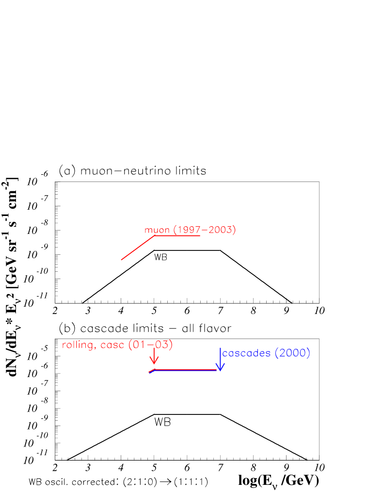
In the diffuse analysis, high-energy (HE) events from all directions are examined with respect to the spectral energy behavior of the sample. A flattening of the total neutrino spectrum at GeV is expected when a flat, astrophysical component () overcomes the steep atmospheric background (). The most restrictive limit is given by the AMANDA experiment, from the diffuse analysis for the years 2000 to 2003,
| (77) |
in the energy range of , see AI+07d .
Diffuse neutrino flux limits are typically obtained by optimizing the analysis cuts on spectra. The dependency of the response function of the detector to different spectra is considered in AI+07d and limits could be set for different spectral shapes (e.g. ) or specific models. Varying the spectral index in the simulation shows that the event distribution simulated for AMANDA peaks at very different energies depending on the assumed spectral index. While, for an spectrum, of the signal lies between for the analysis presented in AI+07d , an spectrum shows an event distribution located about an order of magnitude lower in energy while an spectrum shifts the sensitivity to higher energies. This shows that it is useful and more accurate to model the spectra according to the predicted shape.
4.5 Detection of extremely high-energy neutrinos
Current neutrino experiments are able to measure the atmospheric neutrino spectrum up to TeV without observing a significant contribution from extragalactic sources AI+07d ; M+ (07); Mün (07). Successor experiments like IceCube and KM3NeT aim at the detection of neutrinos at TeV up to PeV. The detection of a signal at even higher energies is restrictedly also possible with IceCube, but to achieve a good detection probability of the cosmogenic neutrino flux, new methods are being developed which are complementary to optical detection. Acoustic and radio neutrino detection aims at the measurement of neutrinos at Extremely High Energies (EHEs), i.e. GeV. In addition, horizontal air-showers or air-showers from rocks, the sea or the Earth are neutrino signatures, since other particles are not able to leave traces through such dense matter. Experiments like Auger, HiRes, MAGIC, etc. can investigate the neutrino flux at energies around GeV by searching for (sub-)horizontal events.
4.5.1 Radio detection
As it was discussed for the first time by Askaryan Ask (62), the Cherenkov effect is not only present at optical and UV wavelengths, but has a strong component in the radio. An electromagnetic shower is caused by a neutrino, produced by interactions of the secondary lepton with electrons from the molecules in the medium. Positrons from pair production annihilate with electrons in the atoms which leads to a negative charge excess of approximately . The shower-size is around cm and the power of Cherenkov radiation is proportional to the frequency and the bandwidth :
| (78) |
The refraction index for light in a medium changes back to at frequencies above the UV light and the differential power decreases. Therefore, Cherenkov radiation is optically seen as blue light. The power is proportional to the squared electrical field,
| (79) |
and for optical frequencies, with N as the number of particles. Thus, the power is proportional to :
| (80) |
For lower frequencies the corresponding wavelength is bigger than the size of the shower and the electromagnetic fields of the particles are in phase. Consequently, the amount of the electric field scales with the number of particles, . Therefore,
| (81) |
The ratio between radio power and optical power of the Cherenkov light is then
| (82) |
Typical frequencies are MHz and MHz and thus,
| (83) |
A particle excess of would be necessary to reach an intensity equivalent to the optical intensity. However, lower efficiencies are sufficient for the observation of the effect: the Askaryan effect was observed for cascade-like events in sand S+ (01), salt G+ (05) and also in ice GA+ (06). While cascade signals result in a significant radio signal as detected, single muons do not radiate enough to be observed. It is used for the purpose of neutrino detection in the RICE313131Radio Ice Cherenkov Experiment experiments which aims at the detection of the radio signal from neutrino-induced cascades at energies of eV in the ice below the geographic South Pole K+ (03). A geometric volume of km3 is instrumented with dipole receivers at a depth of 100 m to 300 m below the surface. The advantage of the high-energy threshold is that the atmospheric background of muons and neutrinos can be neglected. The challenge is the very small signal rate at such high energies. So far, no neutrino signal could be identified yet. Most recent studies concerned the search for individual GRBs, with limits to GRB afterglow neutrino emission models given in B+07b . A second detector trying to measure the radio signal from neutrino-induced cascades is the ANITA323232ANtarctic Impulsive Transient Antenna Experiment balloon-borne experiment BA+ (06), sensitive in the energy range of eV. Radio emission arising from neutrino interactions with nucleons in the Antarctic ice sheet is measured from above. First limits come from test-flights of ANITA-lite, the first full ANITA flight was successfully done in December 2006, with 3.5 circles around Antarctica, with no results published yet. ANITA is expected to investigate the model of GZK neutrinos, either confirming a positive signal, or setting limits which will restrict source evolution scenarios for the production of ultra high-energy protons, see Section 9.1.
Next generation detectors of radio emission from neutrino-induced cascades are planned in salt and in ice. In ice, the AURA333333Askaryan Underice Radio Array experiment GME (93) will be succeeding RICE. The final aim is the instrumentation of a surface of about km3 in Antarctica. A new project using radio antennas on top of the Ross Ice Shelf at the Antarctic coast is ARIANNA343434Antarctic Ross Iceshelf ANtenna Neutrino Array Bar (06), making use of neutrino-induced radio emission in the ice shelf. Salt is a good target material, since it has about times the density of water and ice, and therefore also provides more than 2 times more nucleons within the same volume. The neutrino effective interaction volume is hence increased. The SalSA353535Salt dome Shower Array experiment is planned, where parts of a salt dome is proposed to be instrumented for the purpose of neutrino detection. First tests are already being done in salt domes V+05b .
Another method of detecting neutrino-induced radio emission is to observe the moon with radio telescopes. The moon yields a good target for neutrino interaction and therefore, an enhanced radio signal is expected from the direction of the moon. Projects investigating this effect are planning to use the WSRT363636Westerbork Synthesis Radio Telescope or SKA373737Square Kilometre Array. The latter is planned to be used in the context of the LUNASKA383838Lunar Ultra high-energy Neutrino Astrophysics using SKA project LUN (08). For an overview of the status of neutrino radio detection methods, see e.g. Sal (06).
4.5.2 Acoustic detection
Detectable acoustic signals are expected to accompany neutrino-induced cascades. While cascades are compact and have high energy densities, which produces the acoustic signal, single muons have too low energy density to be detected as acoustic pulses. An estimate of the thermal energy deposit and the energy densities is given in Lea (79). The SAUND393939Study of Acoustic Ultra high-energy Neutrino Detection VGL (05) experiment was the first array built for acoustic neutrino detection. It makes use of a military basis in the Bahamas, located between depths of m and m, spread over a surface of km2. First results were presented in VGL (05). The acoustic technique in the ocean is also tested at the ANTARES site with the AMADEUS404040ANTARES Modules for Acoustic DEtection Under the Sea detector, currently being deployed along with the ANTARES strings N+ (06). The main aim of these prototype detectors is the study of the background and general water properties. For the detection of an EeV neutrino signal, an extremely large array ( km2 surface area) needs to be deployed. In addition to water, ice and salt are good environments occurring naturally for the installation of a large volume acoustic neutrino detector. In the SPATS414141South Pole Acoustic Test Setup project B+ (05); AI+06a , first hydrophones were deployed on three IceCube strings as of December 2007 in order to test the acoustic properties of the Antarctic ice. The final aim is again the construction of a km2 array, in a depth of m, for the detection of EeV neutrinos. For a summary of the current status of acoustic neutrino detection arrays, see Van (06).
4.5.3 Detection of neutrino-induced air showers
The hadronic and electromagnetic cascades which are produced in neutrino-nucleon interactions via the neutral and charged current can also be observed as air showers, in particular in the case of tau neutrinos. Neutrino-induced showers can be distinguished from regular Cosmic Ray showers by choosing events which originate from close to or below the horizon. While Cosmic Ray showers are absorbed by Earth, showers from Earth-skimming neutrinos are induced in the outer mantle of the Earth and propagate further through the atmosphere. Neutrinos traveling through the core of the Earth are attenuated and only nearly horizontal events can be observed as inclined air showers, see e.g. Zas (05). Searches for neutrino-induced air showers are performed by the Cosmic Ray detectors, e.g. by Auger AA+07b and HiRes MH+ (07). A Cosmic Ray Tau Neutrino Telscope (CRTNT), dedicated to the detection of neutrino-induced air showers, is proposed with possible locations in Tibet near the ARGO-YBJ array H+ (07). Cherenkov telescopes with the primary aim of TeV photon showers are also performing neutrino-shower analyses, see e.g. MAGIC GM+07b . The detection of the radio signal from air-showers as planned by the LOFAR424242LOw Frequency ARray experiment F+ (06) also gives the possibility for neutrino detection with a threshold energy of eV S+07a . At these highest energies, exotic particle decays, like topological defects, can be tested. The energy threshold is too high for neutrino fluxes as produced in AGN or GRBs, since the maximum neutrino energy lies below eV. The detection of neutrino-induced radio showers from the moon has similar a detection threshold and is investigated by experiments like FORTE434343Fast On-orbit Recording of Transient Events, GLUE444444Goldstone Lunar Ultra High-Energy Neutrino Experiment and NuMoon.
4.6 Hybrid arrays
The combination of different experimental techniques in one experiment or at the same location has been proven to help the understanding of the fundamental processes to be measured. The latest example is the Auger experiment which uses the complementary pieces of information about the air shower from both fluorescence and surface detectors. Events can be reconstructed with higher accuracy and systematic errors can be reduced. A similar approach done with the combination of IceCube and IceTop Gai (06). Surface stations are deployed together with the IceCube strings in order to measure the electromagnetic component of air showers at the surface in combination with the high-energy muons in the air showers in IceCube. High-energy muons originate from the fragmentation region of hadronic showers, which is not well known Gai (06). The combination of a surface array with an underground muon detector gives a good energy resolution, while the measurement of low-energy muons at the surface provides a better mass resolution, see e.g. Gai (06).
In the case of neutrino detection, the three techniques optical, acoustic and radio detection of neutrinos provide complementary information on the neutrino-induced showers. Therefore, the best reconstruction of single neutrino events will be possible, if all three detection methods are combined in a hybrid array. First simulations of a combined array of acoustic, radio and optical array have been done for ice BI+ (05). Here, the IceCube configuration is used together with a further outer ring of strings for optical detection, as well as an acoustic and radio array with a diameter of km around IceCube. A scheme of the configuration and of the effective volumes of the three arrays and the combined array is given in V+05a .
4.7 Current diffuse neutrino flux limits
In order to optimize the signal to noise ratio, it is useful to assume a certain spectral shape for the potential extraterrestrial contribution. This way, specific cuts can be applied in the data in order to reduce the background as much as possible while keeping most of the signal. Extraterrestrial neutrinos are typically believed to have a spectral behavior close to , and thus, limits are usually derived assuming an spectrum. Table 6 lists current neutrino flux limits, organized according to the lower value of the energy range. All limits are given for a confidence level, except for the RICE results, where confidence level values are quoted. It is important to note that the different experiments are sensitive to different neutrino flavors. It is typically assumed that the flavor ratio for extraterrestrial neutrinos is . Therefore, single-flavor limits can generally be scaled to all-flavor limits by applying a factor of . However, since the flavor ratio of is not exact and can even change significantly at energies above TeV KW (05), the limits are quoted as given by the different experiments, see references in the table.
| experiment | flavor | t | energy range | Ref |
|---|---|---|---|---|
| [GeV] | ||||
| Fréjus | RD (96); D+ (95) | |||
| AMANDA | AI+07d | |||
| Baikal | AB+06b | |||
| AMANDA | M+05c | |||
| AMANDA | AI+07e | |||
| RICE | KR+ (06) | |||
| Auger | AA+07b | |||
| HiRes | MH+ (07) | |||
| ANITA-lite | BA+ (06) |
Specific models can also be tested by changing the signal expectation from an spectrum to a specific spectral shape. Such limits have been set by e.g. AMANDA in the case of muon neutrinos AI+07d and all flavors AI+07e and Baikal AB+06b . It is also possible to derive differential, model-independent limits with methods as described in KR+ (06). These typically trace the energy-dependence of the detector’s sensitivity, giving best results at the maximum performance energy, see e.g. results from GLUE G+04a , FORTE L+ (04) and NuMoon S+07a .
During the past decade, neutrino limits could be improved from values of at TeV energies (Fréjus) to four orders of magnitude lower values, reaching limits as low as at PeV energies (AMANDA). With IceCube, it will be possible to further improve this value by one order of magnitude within only one year of full operation, and up to two orders of magnitude in less than five years, giving the opportunity to detect the first extraterrestrial neutrinos at PeV energies.
5 Galactic sources
The basic assumptions for neutrino production in galactic sources are the same as for extragalactic neutrino sources: in the case of optically thin sources, TeV photon emission can be directly correlated to neutrino emission in the case of a hadronic acceleration scenario. In addition, the emission at lower energies can be interpreted as an avalanched high-energy signal. One striking difference between galactic and extragalactic neutrino spectra is the maximum energy, since galactic sources produce maximum proton energies of eV which is mirrored in the neutrinos’ relatively low maximum energy. Candidates for neutrino emission are the following source classes, which are also listed in table 7.
-
•
Supernova Explosions
Supernova Explosions release a large amount of their energy via the emission of MeV neutrinos. This phenomenon was observed for the first time for SN1987A. Today’s neutrino detectors have created an early warning system for such explosions in our galaxy, the SuperNova Early Warning System (SNEWS) A+ (04). Since neutrinos are emitted prior to the optical eruption, the SNEWS network can trigger optical, radio, X-ray and other telescopes which would probably miss the explosion otherwise. On average, a supernova explosion is believed to happen within our galaxy about every thirty years.
Apart from the thermal neutrino emission prior to the optical outburst, a TeV-neutrino flux is expected to arise from proton-nuclei interactions in Type-II supernova explosions as described in WL (01). Protons are believed to be accelerated in shock-fronts up to proton energies of TeV, resulting in a neutrino flux up to neutrino energies of TeV. -
•
Supernova remnants
Young supernova remnants make up of the dominant part of the charged Cosmic Ray spectrum GS (64). Neutrinos are expected to be produced in the shocks of both shell-type SNRs, see e.g. AlH (02), and plerions, see e.g. GA (03).
The observation of TeV emission from the shell can be interpreted as a signal from decays. The spectral information from the shell-type SNRs and from plerions can be used to calculate the neutrino signal, see K+ (07). The event rates for the single sources are of the order of events in a cubic kilometer detector with a lower energy threshold of TeV, at a rate of atmospheric neutrinos of the same order or even higher. This implies that an effective background rejection is necessary, possibly by performing a stacking analysis in order to observe a significant signal. -
•
Microquasars
Neutrino emission from jet-disk like microquasars was suggestedin Bed (05). Here, it is proposed that nuclei being accelerated in the jet of the system interact with the accretion disk of the compact object or directly with the accompanying Wolf-Rayet star. While photons are absorbed in the dense star or accretion disk, most neutrinos traverse the objects and escape the production region without significant energy loss. The same kind of processes can happen with B- and O-type stars instead of the Wolf-Rayet star.
The detection of a periodic TeV photon signal from the two microquasars LS 5039 and LS I 61+303 encourages models predicting high-energy neutrino emission from massive star/compact companion-type binaries. If the TeV photons are produced in photohadronic interactions, the neutrino signal is directly correlated to the TeV photon signal as described in TH (07). A model presented in Böt (07) predicts an anti-correlation between very high-energy photons and neutrinos. While the region is optically thin in the high-state of high-energy photon emission, it is optically thick in the low-state, allowing for the production of high-energy neutrinos. -
•
Soft gamma repeaters and anomalous X-ray pulsars
Most peculiar events in our galaxy are the so-called soft gamma repeaters or, if the detection is in X-rays rather than in soft gamma-rays, the anomalous X-ray pulsars. Their emission is irregular and does not follow a periodic structure. In addition, the intensity of the flares varies immensely. Low-intensity flares are typically thermal, while the most intense flares have a non-thermal component. The latter are therefore good candidates for neutrino emission. The neutrino emission from the giant flare of SGR 1806-20 was calculated in HLM (05). This flare had a total energy release of erg, which is several orders of magnitude above typical flaring states. The non-thermal photon spectrum is extrapolated to TeV photon energies in HLM (05), assuming that the TeV signal is proportional to the neutrino luminosity. A detection rate of a few events is expected in a cubic kilometer array for such a giant flare. -
•
Molecular clouds and diffuse TeV emission
Molecular clouds have been observed by H.E.S.S. Aha+06g . These are good candidates for neutrino emission: TeV emission is observed, since an astrophysical accelerator hides behind the clouds. The protons are absorbed by the dense clouds (cm3) and produce TeV photons and high-energy neutrinos through proton-proton and proton-photon interactions. Recently, MILAGRO454545Multiple Institution Los Alamos Gamma Ray Observatory detected diffuse TeV photon emission from the Cygnus region GM+ (06). This is a good candidate for a neutrino production site as well as pointed out in HO (07).
So far, only the outer part of the galactic plane can be observed thoroughly, since the most sensitive instruments, AMANDA and IceCube are located in the southern hemisphere. Due to the detector location, the northern hemisphere is visible (see Section 4). With KM3NeT to be built in the north, the southern hemisphere and therefore galactic center will be observable. The remaining challenge is the small maximum neutrino energy, TeV. For a dedicated summary of galactic neutrino sources, see BBM (05).
| source class | origin | normalization | model(s) | |
|---|---|---|---|---|
| SN explosion | ||||
| shocks | em. luminosity | TeV | WL (01) | |
| Shell-SNR | ||||
| pulsars | Cosmic Rays | TeV | BS (75); Sat (77) | |
| diffuse | TeV photons | TeV | K+ (07) | |
| RX J 1713.7-3946 | TeV photons | TeV | AlH (02) | |
| Plerions | ||||
| identified sources | TeV photons | TeV | GA (03) | |
| Crab | TeV photons | TeV | BP (97) | |
| Microquasars | ||||
| jet | jet-disk symbiosis | TeV | Bed (05) | |
| LS I 61+303 | TeV photons | TeV | TH (07); Böt (07) | |
| SGRs&AXPs | TeV photons | TeV | HLM (05) | |
| Cygnus-region | TeV photons | TeV | HO (07) |
6 Neutrinos from Active Galactic Nuclei
The most luminous, persistent objects in the sky are Active Galactic Nuclei. In hadronic acceleration models, it can be assumed that for each class of AGN, the electromagnetic emission is correlated to a neutrino signal. Apart from individual normalization factors, the corresponding cosmological integrations are basically mathematically identical. In this section, the correlation between the emission of neutrinos and photons at different wavelengths will be reviewed according to neutrino flux models which are currently being discussed in the literature.
6.1 Calculation of a diffuse neutrino flux
The total diffuse neutrino spectrum from a certain source class at Earth is given by the single source spectrum convoluted with the redshift and luminosity dependent source number. A factor ) is applied to account for the decrease of the source flux with the luminosity distance . The number of sources is given by the product of the luminosity function of AGN, , and the comoving volume . Thus, the total diffuse neutrino flux can be written as
| (84) |
A shift of the neutrino energy at the source to lower energies at the detection site due to the expanding Universe, is taken into account. A simple cosmology of and is still used for many models, since most spatial distributions of the source samples were given according to this cosmology at the time of the publication of the models. The changes in the normalization of the result when using the experimentally confirmed model of and S+07b should be negligible, as pointed out in DP (90).
6.1.1 Different classes, different normalization options
The overall normalization of the neutrino spectra builds on the correlation between the observed flux from photons or charged Cosmic Rays as discussed in Section 3. In the following section, the prevailing diffuse neutrino flux models are discussed. Table 8 summarizes the different models with their very basic assumptions. Figure 20 shows a selection of the models in comparison with current AMANDA data and the atmospheric prediction.
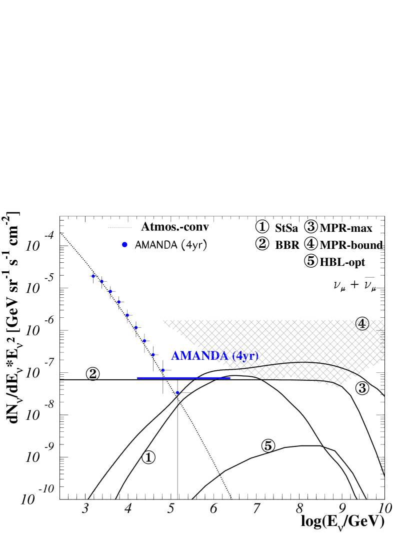
| source class | Normalization | correlation | origin | model(s) |
| wavelength | to wavelength | |||
| blazars | CRs | proton flux, responsible | jet | MPR (01) |
| for in source | M+03b | |||
| MeV | cascaded signal | jet | MPR (01) | |
| connected to | M+03b | |||
| production (s) | Man (95) | |||
| MeV | cascaded signal | jet | Man (95) | |
| connected to | Ste (05) | |||
| FSRQs | radio | jet-disk correlation | jet | BBR05a |
| radio total power | ||||
| FR-II | radio | jet-disk correlation | jet | BBR05a |
| radio total power | ||||
| radio quiet AGN | X-ray | cascaded signal | disk | StS (96) |
| NMB (93) | ||||
| AM (04) |
6.1.2 TeV blazars
Sources of electromagnetic TeV emission can be interpreted as optically thin to photon-neutron interactions, , in hadronic acceleration models M+03b ; MPR (01). In such a scenario, charged Cosmic Rays (CRs) are produced in the vicinity of the source through the decay of the escaping neutrons. In this case, the resulting neutrino energy density would be proportional to the extragalactic CR component measured at Earth. The neutrino flux from High frequency peaked BL Lacs (HBLs) was calculated using the connection between Cosmic Rays and neutrino emission, see M+03b . The neutrino emission peaks at very high energies, i.e. GeV. Due to the low intensity of the signal, it will be difficult to detect such a contribution. A theoretical upper bound of such a contribution to the diffuse neutrino flux was derived by Mannheim, Protheroe and Rachen (MPR bound), see MPR (01) and Fig. 20.
As discussed in Section 3, the high-energy photon tail is absorbed by the extragalactic background light. Therefore, only the local Universe can be observed with TeV photons. The most distant source observed by IACTs so far is 3C 279 at a redshift of , detected with the MAGIC telescope PM+ (07), which is considered as the VHE photon horizon here. In the following, it is assumed that the sources can be observed to this maximum redshift. Neutrinos, being co-produced with TeV photons in hadronic scenarios, offer the possibility to observe the same source classes, but without any losses. The spectra to be observed at Earth correspond to those emitted at the sources, only shifted in energy by . The neutrino flux, originating from the local sources, which can be observed in coincidence with TeV photon experiments, is a factor of smaller than the total neutrino flux. The absorption factor is determined by calculating the ratio of the neutrino flux up to the first formation of galaxies and the total neutrino flux up to ,
| (85) |
The total diffuse neutrino flux cannot exceed flux limits as determined from AMANDA data, the most stringent one being
| (86) |
as presented in AI+07d . Therefore, the flux which can be observed simultaneously in TeV photons and neutrinos is restricted to
| (87) |
The absorption factor is presented in B+07a with values of and . Assuming a horizon for TeV photon detection of or results in a maximum flux of
| (88) |
and
| (89) |
respectively. This result implies that the diffuse fluxes to be observed in both TeV photons and neutrinos are relatively small, even for IceCube prospects. It emphasized the importance of neutrino analyses independent of photon measurements, such as the general diffuse search, see e.g. AI+07d ; Mün (07).
6.1.3 EGRET and COMPTEL blazars
In the case of optically thick sources (), the TeV photons from decays interact with nucleons in the source before escaping at lower energies leading to the emission of sub-TeV photons. Therefore, the diffuse extragalactic background measured by the EGRET464646Energetic Gamma Ray Experiment Telescope experiment SMR (05) ( MeV) can be interpreted as an avalanched TeV signal from blazars and can thus be used to normalize the neutrino flux from EGRET or COMPTEL474747COMpton TELescope-type sources. Again, an upper bound to the contribution from such sources is given in MPR (01), which is much less restrictive than the optically thin case. Apart from the bound, a calculation of the maximum contribution from blazars is given in MPR (01). In addition to the contribution from HBLs given in M+03b , a contribution from the optically thick Low-frequency peaked BL Lacs (LBLs) can be calculated using the EGRET diffuse extragalactic background for a normalization of the neutrino spectrum, see M+03b . A model of proton-photon interactions in AGN and collisions of protons from the core with protons of the host galaxy is derived in Man (95). For sources with an even higher optical thickness, only photons below MeV escape. In this case, the neutrino signal can be normalized to the diffuse extragalactic contribution measured by COMPTEL at energies in the range of MeV K+ (96). This would enhance the contribution of neutrinos from proton-photon interactions by almost an order of magnitude as shown in Man (95).
A model by StS (96) was originally using the diffuse cosmic X-ray background and has recently been modified in a way that it is using the COMPTEL diffuse background to normalize the neutrino spectrum Ste (05), see Fig. 20. This reduces the formerly very high contribution by a factor of 10. In addition, oscillations have been taken into account which leads to a further reduction by a factor of 2.
6.1.4 X-ray detected AGN
The measurement of the diffuse extragalactic contribution in X-rays by ROSAT484848ROentgen SATellite has raised the question whether it is produced by radio-weak AGN. Assuming that the X-ray emission comes from the foot of the jet, the X-ray signal would be accompanied by a neutrino flux. A model by NMB (93) and an approach by StS (96) have been presented, predicting a correlation between X-ray emitting AGN and neutrino emission from the same sources. In these models, interactions produce high-energy photons, which cascade down to X-ray energies before escaping due to the optically thick environment. An alternative scenario for the explanation of the X-ray flux from AGN would be the up-scattering of thermal electrons via the Inverse Compton effect. In that case, the X-ray component would not be accompanied by a neutrino signal, see e.g MSR (95). Until today, about of the diffuse X-ray signal has been resolved by ROSAT BH (05), with the help of Chandra and XMM-Newton494949X-ray Multi-Mirror Mission Newton data, this number can be updated to , see BH (05) and references therein. More than of the diffuse background are possibly connected to the X-ray emission of Active Galactic Nuclei most of which are radio weak. The search for a diffuse, extraterrestrial neutrino flux with AMANDA did not yield a significant signal and restricts these models strongly.
6.1.5 FR-II galaxies and FSRQs
The diffuse neutrino flux from FR-II galaxies using average parameters has been calculated in BBR05a . For the derivation of a source spectrum, it is assumed that the neutrino spectrum follows the proton spectrum in first order approximation. Effects from multi-pion production are neglected. The changes to the spectrum due to this effect would be negligible with respect to other remaining uncertainties in the calculation, such as the lack of knowledge of the sources’ optical depth. For the normalization of the spectrum, it is assumed that the neutrino output of a single AGN is proportional to the total power of the jet given by the disk luminosity BBR05a . The disk luminosity is linked to the radio output via the jet-disk symbiosis approach which was developed in FB (95); FMB (95); Fal (96). The spectral behavior is generically chosen as , with a resulting spectrum of
| (90) |
for one neutrino plus anti-neutrino flavor, including oscillations. Here, is the effective optical depth to interactions.
With the currently most restrictive flux limit, see Equ. (86), the optical depth has to be smaller than . The maximum flux for is shown in Fig. 20. The limit, however, only applies if the spectrum does not deviate strongly from the shape. It was pointed out by different authors, e.g. Bar (04); MBQ07b , that the spectral shape can vary significantly under certain conditions of relativistic shocks. While flatter spectra may still be excluded by the limit, steeper spectra are more difficult to investigate. When interpreting the radio spectrum as synchrotron radiation from electrons, the radio spectral index is correlated to the primary index as . The neutrino spectrum, following the proton spectrum, could therefore be as steep as .
6.2 Individual source spectra
For the calculation of the diffuse spectra discussed above, mean parameters have been used. In this section, different predictions implementing the individual variations of the single sources are discussed.
6.2.1 TeV emitters
A simple estimate of the neutrino flux from TeV sources is to use the photon flux at TeV energies under the assumption that it arises from photo-hadronic interactions. It is known that the TeV photon flux is diminished by interactions with the extragalactic background light. Thus, the TeV photon flux at Earth and its spectral index are used here as a lower limit for the photon emission from the blazars. The neutrino flux is given as
| (91) |
with the spectral index . The normalization factor is calculated by correlating the neutrino flux luminosity with the TeV photon flux as
| (92) |
Here, for interactions and for interactions, see e.g. Hal (06). Assuming that the spectral indices for neutrino and TeV photon emission and the energy threshold ( GeV) are about equal translates the above equation into a direct correlation between the flux normalizations,
| (93) |
Table 9 lists the normalization for the neutrino spectrum of the 13 HBLs with given spectral information, the LBL BL Lacertae and M 87. The values have been calculated using the parameters in table 2 in Section 3. The results are listed for a correlation between photons and ()-neutrinos as it is the case for proton-proton interactions. Dividing the values by 4 yields the flux in case of interactions. It needs to be considered that the TeV photon flux from blazars is highly variable. The intensity of the low state can be several orders of magnitude below the high-state flux. Both difficulties and opportunities arise from the strong variability.
The estimated neutrino signal from high-state photon states in AGN and point source neutrino flux limits as given in AI+07b for 6 of the individual sources are listed in table 9. However, the limits cannot directly be compared to the estimated flux: the calculated values are only valid during the time of the flare, while the limits apply to the flux averaged over the five years of observation. The latter is significantly lower and for many of the TeV sources, the low-emission state is not known. Low-state observations require long observation times. The duty cycle of Cherenkov telescopes is quite low, since only dark nights can be used for measurements. Therefore, extensive long-term monitoring of the sources is not possible with the current telescopes. Many flares are missed and the average flux is difficult to determine. Small telescopes, dedicated to the long-term monitoring of TeV blazars, are planned to be rebuilt from HEGRA telescopes as described in BM+07b . Currently, the Whipple telescope uses part of its time for blazar monitoring in order to get a better estimate of the TeV lightcurve SV+ (07). These attempts may be an option to get a better understanding of the variability of the sources. The small telescopes are, however, typically not sensitive to low-state emission. This has to be examined by the more sensitive telescopes, H.E.S.S., MAGIC, VERITAS & co.
The flaring states also provide an advantage for high-energy neutrino telescopes: for known flares like the ones listed in table 9, temporal cuts in the data of neutrino telescopes can be used in addition to spatial cuts. If only the duration of the flare is used for an analysis, the estimated flux values can be used as reference values. This way, a much higher flux is expected, in addition to a reduced background, which increases the probability of detecting a signal. Analysis methods concerning AGN flare searches are being developed as presented in RI+ (06).
| Source | year | (flare) | Limit |
|---|---|---|---|
| (TeV obs) | TeV-1 s-1 cm-2 | TeV-1 s-1 cm-2 | |
| M 87 | 2005 | 11.7 | 440 |
| Mkn 421 | 2001 | 311 | 370 |
| Mkn 501 | 1997 | 1001 | 740 |
| 1ES 2344+514 | 1995 | 510 | 300 |
| Mkn 180 | 2006 | 12.0 | - |
| 1ES 1959+650 | 2002 | 740 | 680 |
| BL Lacertae | 2006 | 3.6 | - |
| PKS 2005-489 | 03/04 | 2 | - |
| PKS 2155-304 | 2006 | 2060 | - |
| H 1426+428 | 2001 | 50.0 | 470 |
| 1 ES 0229+200 | 05/06 | 6 | - |
| H 2356-309 | 2004 | 3.00 | - |
| 1ES 1218+304 | 2005 | 12.7 | - |
| 1ES 1101-232 | 2006 | 4.44 | - |
| 1ES 0347-121 | 2006 | 4.5 | - |
| 1ES 1011+496 | 2006 | 3.2 | - |
| PG 1553+113 | 05/06 | 2.1 | - |
6.2.2 FR-II galaxies and FSRQs
A sub-sample of 114 FR-II sources from the steep spectrum sample given in W+ (01) was used to analyze the differences between an average prediction and a source property based estimate, see BBR05b . The radio flux is converted into the radio luminosity as
| (94) |
and the spectral radio index is used to determine the proton spectral index for each case individually, . The single source normalization versus the primary spectral index is shown in Fig. 21. The normalization is given at GeV. There is a strong correlation showing that flat neutrino spectra are stronger than steep ones. The coincidence spectrum is much flatter than the average prediction,
| (95) |
Using the mean spectral index results in a much steeper mean spectrum due to the correlation between the normalization and the spectral index .

6.3 Theoretical upper bounds on neutrino emission
An upper bound on the diffuse neutrino flux from extragalactic sources was derived in WB (99). Here, the observed spectrum of UHECRs was used in order to calculate the maximum neutrino flux possible to be produced together with the highest energy Cosmic Rays. The bound is given as
| (96) |
for muon and anti-muon neutrinos. It is pointed out in MPR (01) that this bound is, however, only valid for sources optically thin to neutron-photon interactions. In those sources, neutrons escape, decay and produce the flux of UHECRs. High-energy photons from proton-photon interactions escape at TeV-PeV energies. The bound derived in WB (99) does therefore not apply to those classes of AGN which are optically thick to neutron-photon interactions. In addition, it is pointed out in MPR (01) that the calculations in WB (99) assume a strict spectrum. The neutrino spectrum, however, deviates from the primary spectrum of charged particles, which needs to be taken into account in the case of the derivation of an upper bound. Taking these facts into account, a bound for transparent sources and optically thick sources was derived in MPR (01) as indicated in Fig. 20. The upper, straight line of the shaded area represents the bound for optically thick sources, while the lower line shows the upper bound concerning optically thin sources.
It is generally very difficult to derive absolute upper bounds. There are still large uncertainties in many of the parameters. Taking for instance the flux of high energy Cosmic Rays, which is uncertain by at least a factor of two, when comparing the results from HiRes and Auger, see Fig. 2. Further uncertainties come from the spectral index of the primary flux and the neutrino flux, the redshift distribution of the different source classes, as well as the factor which connects UHECRs or photon emission with neutrinos.
6.4 North and south view - next generation neutrino detectors
Both for point source and diffuse searches, the orientation of the field of view of the detector is crucial. The sources are not distributed isotropically. Sky surveys can be biased by the location of the instruments and the brightest source in a sample sometimes makes up the dominant contribution from a source class. The latter is, for instance, the case for FR-I galaxies, where M 87 gives most of the radio flux in the total sample. The reason is that M 87 is by far the closest of the sources, at a distance of only Mpc.
The measured diffuse flux depends on the location of the detector. If the luminosity distribution is steep, implying that nearby sources make up most of the contribution, the signal is much stronger with the nearby sources in the field of view.
IceCube is currently being built at the geographic South Pole with a full view on the northern hemisphere in the muon-neutrino channel. The complementary instrument, Km3NeT, planned to be built in the Mediterranean, will cover the southern hemisphere. Depending on the source class, optimal observation conditions are provided by either southern or northern telescopes. For instance, in the case of EGRET-detected sources, the three brightest objects are in the southern sky. The largest fraction of identified FR-I and FR-II galaxies are located in the northern hemisphere, since the supergalactic plane is mostly located in the northern hemisphere and there may also be a bias in the radio selection of objects. A detailed description of the most important catalogs is given in B+07a .
6.5 Physics conclusions from current neutrino flux limits
The primary goal of large volume neutrino arrays is the detection of a signal from extraterrestrial sources. Different methods have been developed in order to reduce the atmospheric background, using the model predictions described above for an optimal selection of data. Here, energy cuts are applied for diffuse searches and spatial and temporal cuts are used for point source searches. The stacking of the most intense objects of a source class can further improve the signal to background ratio. This was done for 11 AGN classes with the AMANDA detector, as described in AI+06b ; AI+07b . Here, typically the ten brightest sources in the sample were used for the analysis. The point source limits can be interpreted as diffuse limits, as described in B+07a ,
| (98) |
The factor includes identified sources contributing to the diffuse flux, which have not been considered in the stacking analysis505050In many samples, most of the sources are too faint to be considered in the stacking analysis - including them would reduce the sensitivity. They still have a significant contribution to the diffuse flux.. The second factor accounts for the diffuse background of unidentified sources. This is only known for some of the source classes and needs to be estimated in other cases. The factor sr accounts for the field of view of the AMANDA detector.
The best results are achieved for identified EGRET blazars. The stacking diffuse limit is given as
| (99) |
in the energy range of TeV TeV. This is not a general diffuse limit, but it only applies for diffuse flux predictions building on a correlation between the photon flux as measured by EGRET and neutrino emission. While the limit cannot restrict current predictions, second generation neutrino telescopes like IceCube and KM3NeT will be sensitive to the prediction of neutrinos from interactions described in Man (95) at energies around TeV. The advantage of the stacking method is that it is sensitive to neutrino fluxes at relatively low energies, while the general diffuse search is restricted to energies of above TeV due to the high atmospheric background.
The diffuse search, on the other hand, is more sensitive in most of the cases at higher energies, since the stacking method loses sensitivity due to the high diffusive factors which can reach values up to in the worst case. With current neutrino flux limits, it is possible to exclude the correlation between X-rays and neutrino emission B+07a . The three predictions, i.e. StS (96); NMB (93); AM (04) show a violation of the limit by about an order of magnitude. It is therefore excluded that neutrinos are produced in coincidence with X-rays from radio-quite AGN. The modified model of Stecker et al. Ste (05), assuming a correlation between neutrinos and MeV photons rather than X-rays is a factor of lower than the original prediction. The factor of arises from the fact that the diffuse MeV flux is lower than the X-ray flux, which translates directly into a lower neutrino flux.
A search for ultra high-energy neutrinos was performed in AI+07e . At energies around PeV, neutrinos are effectively absorbed by the Earth and only reach the detector when coming from close to the horizon. Events from above are difficult to distinguish from atmospheric muons, which leaves horizontal neutrinos for the analysis. The limit for three year of data taking (year 2000-2003) lies at
| (100) |
Limits have been derived according to different models. The limit lies a factor of below the prediction of MPR (01), presenting the maximum contribution from optically thin sources. The most optimistic parametrization can therefore be excluded. With IceCube, a sensitivity gain of about two orders of magnitude in one year of observation is expected, providing more information on the parameters of different flux models at high energies.
6.6 The Olbers’ paradox for neutrinos
First predictions of high-energy neutrino emission were made in the 1990s with maximum parameter settings in order to estimate what is possible. These models could now be revised using more realistic parameters due to current neutrino flux limits. While it is obviously the aim to detect high-energy neutrinos from extraterrestrial sources, the limits which have so far resulted from the searches are very valuable in the context of multimessenger astrophysics as discussed above. These limits are in analogy to the Olbers’ paradox. The paradox arose when Olbers calculated that - with a homogeneous distribution of astrophysical objects in the sky, and with these objects radiating isotropically - that the sky should be isotropically bright as the sun itself Olb (26). There was, however, a very obvious, optical limit on the radiation during night-time. The sky was, and still is, dark! The paradox could not be solved before the 1950s, when different assumptions from Olbers’ calculations fell: the sources are not isotropically distributed in the sky, the Universe is not infinite and it is not in thermal equilibrium.
Similar considerations can be done for every other wavelength, where a prediction is made which violates experimental limits. The limits give the opportunity to constrain the parameters of the model. With neutrino-astrophysics, we are still at the beginning of exploring these predictions. Still, current neutrino flux limits start to become sensitive to prevailing neutrino flux models and start to constrain them. Within a short time, the next generation of large volume detectors will be able to reach sensitivities more than orders of magnitude better than current instruments and it can be expected, that the first extraterrestrial neutrinos will be detected soon.
7 Gamma Ray Bursts as neutrino sources
A summary of the photon and neutrino emission from GRBs is shown in Fig. 22. Three phases of non-thermal emission are expected, i.e. precursors hours prior to the GRB RMW (03), emission during the prompt phase WB (97, 99) as well as afterglow emission WB (00). The lower row shows the neutrino energy spectra for the three phases while the upper row displays the corresponding electromagnetic output schematically.
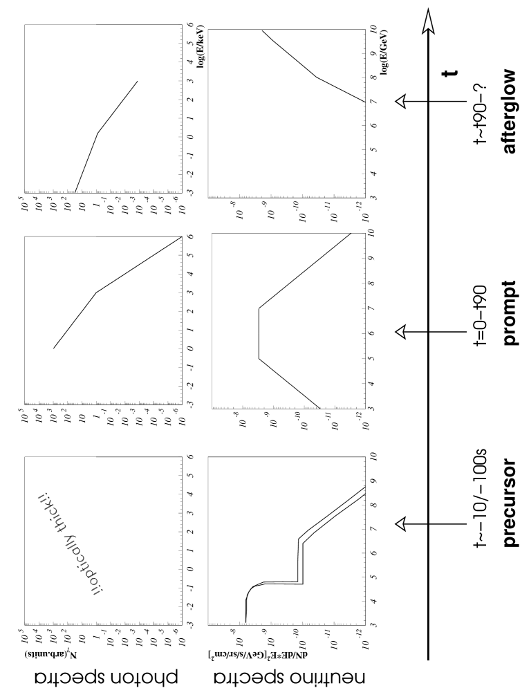
-
•
A precursor model has been developed in RMW (03). The basic idea is that a shock forms when the pre-GRB matter collides with the wind of the central pulsar or the SNR shell. At this point, the burst is still opaque to photon emission and the shock environment yields a good target for neutrino production by shock-accelerated protons interacting with thermal X-rays in the sub-stellar jet cavity. The shocks happen at smaller radii than the prompt emission and at lower boost factors . The neutrino signal could also be accompanied by a signal in the far infrared. The low energy part of the neutrino spectrum arises from neutrino production in interactions and is -shaped. The flux at energies GeV originates from proton-photon interactions. The two lines in the lower left panel of Fig. 22 represent different shock/jet radii and envelope mass settings.
-
•
The prompt photon emission from GRBs can be correlated to the observed flux of UHECRs, since protons are believed to be accelerated in the highly relativistic shocks Vie (95); WB (97, 99). The acceleration of protons in turn implies the production of neutrinos through photon-hadronic interactions. The resulting flux is shown in the lower middle graph of Fig. 22.
-
•
Afterglow neutrinos are produced when the internal shocks from the original fireball hit the interstellar medium and produce externalshocks WB (00). As for the prompt emission, the synchrotron emission of electrons gives evidence for the existence of relativistic charged particles which in turn implies neutrino production by the baryonic component of the jet and the photon field. In the case of afterglow emission, Waxman and Bahcall WB (00) predict the acceleration of ultra high-energy protons ( eV) in reverse, mildly relativistic shocks MR (97). The acceleration of protons to such high energies implies the production of neutrinos in proton-photon interactions in environments optically thick to proton-photon or proton-proton interactions. Waxman and Bahcall conclude in WB (00), that a significant neutrino flux during the afterglow phase is directly correlated to the electromagnetic afterglow emission.
The three different emission phases are discussed in more detail in the next paragraphs. All variables are given in the observer’s frame.
A general question is the timing of photon and neutrino emission. Depending on the environment of the astrophysical shock, neutrinos are not exactly emitted at the same time as the photons. This is important in the case of temporal selection of data in high-energy neutrino experiments. It is typically still assumed that flaring sources emit neutrinos during the same time interval, but the time window is often chosen to be slightly larger than the photon emission time to account for this effect. Transient astrophysical shocks in the context of temporal evolution are described in RM (98).
7.1 Precursor neutrino emission
Since the observation of GRB980425 and GRB030329, it is known that at least a fraction of long GRBs originates in heavy supernova explosions, see e.g. M+03a . The emission is beamed, so that not every supernova explosion can be observed as a GRB as well. The Gamma Ray Burst can only be detected when the jet is directed towards Earth. The pulsar, remaining in the center of the SNR, is believed to form prior to the GRB. The pre-GRB is propagating outwards, and a shock is formed when it meets the magneto-hydrodynamic pulsar wind. In this shock, protons can be accelerated. The fast protons in turn interact
-
1.
with the supernova remnant’s photon field,
-
2.
with the photon field of the MHD wind itself, and
-
3.
with cold protons from the slow plasma.
In the these interactions, neutrinos are produced RMW (03). The total spectrum is calculated by assuming that a fraction of the fast proton spectra, , are converted into neutrinos,
| (101) |
Here, is the luminosity distance and GeV is the threshold energy of the protons for the production of the -resonance. Below this threshold, interactions dominate, where is the proton-proton efficiency. Above the threshold, the total spectrum is given by neutrinos generated in interactions. For the case of photo-hadronic interactions, the proton spectrum needs to be weighted by the fraction of protons converted into pions, , and it needs to be considered that the flux distributes equally to the four decay products . For the case of proton-proton interactions, it needs to be considered that the neutrino multiplicity for an incident proton, , is energy dependent as
| (102) | |||||
Here, is a step-function, which is for the given range and elsewhere. The product is the lower energy threshold for pion/kaon production, with as the mass of the particle and as the Lorentz boost factor at the center of mass in the lab-frame. The normalization factors or are given by integrating the distribution of pions, resp. kaons. The total numbers are given as and . The proton-proton efficiency is assumed to be , see RMW (03).
The proton spectra are calculated in RMW (03), assuming an shaped spectrum. The resulting flux is shown in the lower left graph of Fig. 22. The precursor is not observable in photons, since the environment is optically thick. Thus, the detection of neutrinos from precursor GRBs in the future provides the possibility to alert photon experiments before the actual GRB occurs. In KM (07), it is proposed to use neutrino events in IceCube as a possible trigger for optical telescopes. If the neutrinos arrive in multiples within a short time window, they might originate from a core-collapse supernova. Such a trigger would allow for the observation of SNe in the early phase of the collapse.
7.2 Prompt GRB spectra & neutrinos
The prompt GRB photon spectrum, , is usually given by a Band fit B+ (93),
| (103) |
Here, is the photon energy, is the reference energy with as the break energy in the photon spectrum. The function was designed empirically in order to match the GRB spectra. It is the best mathematical description for broadband GRB spectra. The energy range of detection may not cover both parts of the spectrum and spectral fits with simpler powerlaw approximations are often applied. The break energy for the photon spectrum is given as MeV.
The spectrum is presumably produced by synchrotron radiation of electrons in the internal shock fronts of the jet, see e.g. HaH (02) and references therein. There are two approaches to explain the break in the spectrum at a break energy of typically keV. The most common explanation is the steepening of the spectrum by one power due to the cooling of electrons at high energies, see for example ZM (04); Pir (05) as a review. The break can also be explained by assuming an Inverse Compton scattering scenario, see e.g. DR (04) and references therein. Throughout this review, all energies concerning GRB spectra are given in the observer’s frame at Earth unless declared otherwise. For a regular GRB, the spectral indices are usually distributed around average values of and . These values scatter over a wide range. Short GRBs tend to have harder spectra with and . Assuming hadronic acceleration in the jet, a prompt neutrino flux that is correlated to the photon spectrum results from photo-hadronic interactions in the source.
The neutrino spectrum, , can be derived assuming that the proton spectrum follows the electron spectrum of the source. Furthermore, it needs to be assumed that electron losses can be neglected. The neutrino flux in turn follows the proton spectrum in a first order approximation, since it can be connected to the observed synchrotron spectrum of the sources. An improvement of the calculations is generally possible by calculating the electron losses You (06). Here, this effect is neglected and the result is taken as a lower limit for the neutrino flux.
Protons accelerated in astrophysical shocks can interact with the source’s photon field and produce a resonance which in turn leads to neutrino production. Proton and neutrino energy are directly proportional, . The product of proton and photon energy remains constant, since the energy of the mass has to be produced in the center of mass system, . Hence, photon and neutrino energy are inversely proportional, . The neutrino flux is then given as
| (104) |
The photon spectral indices can be used to describe and . It should be noted that the usage of a broken powerlaw instead of the original Band function can lead to increased uncertainties in the calculation as pointed out in TD (07). The use of the original Band function is more accurate, since it is able to fit the GRB spectrum very precisely over the whole energy band, keV. A complete Band fit, however, cannot be extracted for many bursts. In the case of BATSE, it was still possible to reconstruct the entire Band function, while with Swift, only single powerlaw fits are possible in most of the cases. Also, in combination with the uncertainties in the measurements, the difference between using a broken powerlaw compared to a Band function may be negligible in many cases. Therefore, for simplicity, a broken powerlaw is used in the following paragraphs for cases where the entire bandwidth is detected.
A second break at appears in the neutrino spectrum which is caused by synchrotron radiation of the neutrino-producing pions. Pions with sufficiently high energies suffer synchrotron losses before decaying and do not produce neutrinos. Thus, the high-energy tail of the neutrino spectrum is steepened by one power,
| (105) |
The spectrum is normalized to the -ray fluence which is assumed to be proportional to the neutrino luminosity,
| (106) |
All parameters occurring in the following calculations are listed in table 10. The factor is given by the product of the energy transferred to the pions, , a factor since half of the photo-hadronic interactions result in four neutrinos and a factor to account for the fraction of total energy in electrons compared to protons in the jet G+04b . The normalization constant is therefore given as
| (107) |
In the following, the normalization of a single burst will be modified to a quasi-diffuse normalization by multiplying with the number of bursts per year ( bursts per year, of which are long and are short) and dividing the result by sr,
| (108) |
This number is comparable to the normalization which is achieved when using the flux of UHECRs to normalize the spectrum, since the power in UHECRs is of the same order as the electromagnetic emission of GRBs. The total number of 1000 bursts per year is chosen to be consistent with calculations given by Waxman and Bahcall in WB (97, 99). A estimate of bursts per year, however, is a more reasonable number when looking at the BATSE catalog P+ (99). In that case, all results could simply be weighted by another factor of .
The first break energy in the spectrum, , is related to the break energy in the photon spectrum by
| (109) |
It is determined through the minimal energy necessary to produce a -resonance in the shock fronts of the bursts. The numerical values given in YP+ (06) for the proton mass, GeV, and the mass, GeV, lead to
| (110) |
in the observer’s frame.
The second break energy is connected to the pion’s synchrotron loss time. It depends on the neutrino flavor and for muon neutrinos, it is given as
| (111) |
with the Thomson cross section cm2 and s as the pion life time at rest. For electron and anti-muon neutrinos, the break energy is about an order of magnitude lower, since these neutrinos originate from muon decays. The muon lifetime is about a factor of 100 higher than the pion lifetime, which gives a lower energy threshold for synchrotron losses. Here, and are the fractions of the burst’s internal energy going into the magnetic field, respectively into electrons. The equipartition fractions have been set to and . There is no good way of determining the equipartition fractions theoretically, yet. However, afterglow observations indicate values on the order of for prompt emission WKF (98). The remaining parameters in Equ. (111) are listed in table 10, with the values as used in the following calculations. Inserting all numerical values gives
| (112) |
A detailed derivation of the neutrino spectrum as presented above is given in WKF (98).
7.2.1 The average spectrum
The average spectrum of prompt neutrinos from regular GRBs was calculated in WB (99), hereafter referred to as WB. The following parameters were used,
| (113) | |||||
| (114) | |||||
| (115) | |||||
| (116) | |||||
| (117) |
Though the sensitivity of current neutrino detectors is not sufficient yet to detect this flux (see also Section 4), they come close to the predicted flux. With IceCube, the model can therefore be tested in detail.
A numerical calculation of the prompt neutrino spectrum from GRBs is given in MN06a . Multi-pion production is included in the calculations by using the GEANT4 generator, and proton cooling was calculated. This more precise approach results in a spectrum similar to the one calculated in WB (99), but with smooth transitions at the break energies and a slightly different normalization.
7.2.2 The parameters
The parameters in the neutrino flux calculations have been adjusted according to the different classes of GRBs. A summary of the mean values of the used parameters is given in table 10, for Gamma Ray Bursts, X-Ray Flashes (XRFs), Short Hard Bursts (SHBs) and Short High-Energy (SHE) bursts. The different source classes are discussed in section 7.2.3.
| Parameter | Symbol | GRB | XRF | SHB | SHE |
|---|---|---|---|---|---|
| fluence | [erg/cm2] | ||||
| Redshift | |||||
| Lumi. dist. | [Gpc] | ||||
| energy | [keV] | ||||
| energy | [GeV] | ||||
| Equipartition | |||||
| fractions | |||||
| energy ratio | |||||
| Energy transferred to | 0.2 | 0.2 | 0.2 | ||
| Burst luminosity | [erg/s] | ||||
| 0.1 | 0.1 | ||||
| Boost factor | 30 | 300 | 3000 | ||
| 0.1 | 1 | 10 | |||
| Spectral indices | |||||
| break energy | [MeV] | ||||
| MeV | |||||
| break energies | [GeV] | ||||
| [GeV] | |||||
| Time variability | [ms] | 10 | 1 | 1 | |
| 1 | 0.1 | 0.1 | |||
| Burst duration | [s] | 40 | 40 | 0.2 | 0.2 |
The boost factor is constrained to for regular GRBs, since for boost factors less than , the medium would be optically thick to photons and for , protons lose most of their energy to synchrotron radiation HaH (02). The possibility of fluctuating using the photon break energy is given as demonstrated in G+04b , but there are several arguments for using a constant value: bursts can be misaligned which would lead to a misinterpretation of the boost factor. Also, varying the break energy for each single burst might implicitly already include boost factor fluctuations. Therefore, a constant boost factor of is used in following calculations.
In previous publications, e.g. G+04b , a variation of the energy going into pions was discussed. Such a variation would further increase the width of the distribution of the neutrino spectrum normalization. The burst luminosity, the boost factor, the photon break energy and the variability time influence , as they are correlated as
| (118) |
In the following calculations, this fraction will be kept at a constant value of for classical GRBs for the following reasons:
-
1.
strongly depends on the boost factor which will be used as a constant as discussed before. The dependence on the other three parameters is only linear. The variation of is more striking, since it is amplified by the behavior.
-
2.
The main uncertainties in the current calculations result from the lack of knowledge of the parameters and as well as from uncertainties in the redshift relation which leads to uncertainties in . These three parameters are all important in the determination of the spectral normalization and thus a constant value is favorable.
In the case of SHBs, the variability time is smaller, and also the luminosity is about an order of magnitude lower, . Thus, the pion energy constant stays the same and is assumed to be for SHBs as well.
X-Ray Flashes (XRFs) will produce very high pion efficiencies due to their low boost factors and break energies. indicates an optically thick source in comparison to a classical GRB and yields a good target for neutrino production.
The prediction of the diffuse neutrino flux derived from the model above is given in WB (97, 99), where the authors use average parameters to determine the shape of the spectrum. Cosmological evolution of the sources was considered in that model by taking into account the redshift evolution of GRBs. It is assumed that GRBs follow the star formation rate, since they appear to be connected to supernova-Ic explosions. Thus, the diffuse Waxman-Bahcall flux has to be weighted by a factor or for long and short burst samples respectively.
7.2.3 Conventional versus peculiar bursts
As discussed in Section 3, GRBs can be divided into different sub-classes, such as long and short events and a further division of long bursts into XRR bursts, XRFs and regular GRBs. While short and long bursts differ in duration and in the hardness of the spectrum, XRR/XRFs and regular GRBs differ in the energy range of prompt emission. A further class of short bursts is predicted with a high-energy component, which has not be observed yet, but which would be observable with GLAST.
The photon spectral properties are reflected in the neutrino spectra. A schematic representation of the neutrino spectra of the four different classes is shown in Fig. 23. Due to a low boost factor of , XRR and XRFs have a lower break energy in the photon spectrum, which leads to higher neutrino break energy, GeV for XRR/XRFs (b) compared to GeV for regular GRBs (a). The second break is at approximately the same energy, GeV due to the combination of a lower boost factor and a higher variability time, due to large emission regions. XRRs and XRFs can actually be very efficient neutrino emitters, given that for the low boost factor, the pion parameter can become as large as . Such a high value of would, however, violate recent AMANDA limits, see Section 3. Therefore, the flux is normalized to the current limit in Fig. 23, which implies that the pion parameter must be . Other possibilities to get around the limit would be to use smaller scales for the emission region and therefore smaller variability time scales. This reduces the synchrotron break energy significantly. Also, there could be much less XRR and XRF events than regular GRBs, which would affect the normalization. The variation of the total luminosity plays an additional role, affecting both the normalization and the second break energy.
The photon spectra of short bursts are typically harder than long ones which leads to a much softer neutrino spectrum of below the break energy and above the break energy (see Fig. 23 (c)). The class of high-energy short bursts would produce a neutrino spectrum as displayed in Fig. 23 (d). There is, however, no experimental evidence yet that such a class exists. While the photon spectrum would be observed at MeV energies, the corresponding neutrino spectrum is supposedly visible at lower energies as indicated in the figure.
The reflections above show that the assumption of a (2:1) ratio of long to short bursts and a (1:1:1) ratio of (GRB:XRR:XRF) would result in a modified spectrum which can look significantly different from the spectrum which has so far been classified as the typical neutrino GRB spectrum.
In addition to the classification scheme as presented above, there are two types of bursts which are of low photon luminosity, but can possibly be sources of a significant flux of high-energy neutrinos: low-luminosity GRBs like GRB060218 and choked bursts. The neutrino flux from low-luminosity GRBs is estimated in M+ (06) to be at a level of at GeV, which would be observable by IceCube after a few years of observation. Neutrino emission from choked GRBs is predicted in MW (01): While the electromagnetic emission is not observed due to the optical thickness of the event, e.g. a supernova explosion into a dense SN-wind, neutrinos from proton proton or proton photon interactions can still escape. Further acceleration of secondary charged particles like muons, pions and kaons can lead to an enhanced neutrino signal KW (07). Proton proton interaction for instance would only produce high-energy neutrinos up to TeV. Assuming further acceleration, the maximum neutrino energy lies above TeV and a flux of is expected for an type neutrino spectrum.
Apart from spectral fluctuations between different burst classes, there are relatively large variations within the classes themselves.

7.2.4 Average versus single source variation
A different approach to predicting the neutrino flux from GRBs is to look at each burst individually and add up the individual spectra to make a prediction of the total flux from these sources. The study of different catalogs are presented in G+04b ; B+ (06); Bec (07) and are summarized here.
For each burst in a sample of GRBs, a prediction of the prompt neutrino flux, , from this source can be made as described above. With a large volume neutrino telescope like AMANDA, a large number of bursts can be analyzed simultaneously in order to increase the detection significance. By stacking many bursts, the signal is increased more than the background. This makes it interesting to look at a coincident spectrum of burst samples, i.e. a quasi-diffuse flux. The total flux is given as
| (119) |
Three different burst samples are used here for a systematic investigation:
-
①
BATSE sample: the energy spectrum of 568 bursts from the BATSE catalog are given in G+04b . The neutrino spectra for the individual bursts was derived in G+04b and in B+ (06) using different parameter settings. Calculations here are following the latter publication B+ (06). Redshifts are determined using the variability method, see FR (00) for a description.
-
②
Konus sample of short bursts: a catalog of 130 short bursts has been presented in M+05a , of which 99 have fitted energy spectra and 34 are localized. Redshifts are set to , if unknown515151Short bursts are believed to occur when neutron-star/black hole binaries merge. These events typically happen in old regions, and the mean redshift is therefore expected to be as low as ..
-
③
Swift sample of long bursts: measurements from Swift-BAT have been published on the Swift web-page Swi (08). In this sample used here, those 188 long bursts with published spectral information until March 12, 2007 are included. For the Swift bursts without measured redshifts, is assumed.

To compare the different samples to each other, the coincidence fluxes of the samples are shown in Fig. 24. Three major conclusions can be drawn from the comparison of coincidence spectra.
-
1.
While the spectral shape for the three samples of long bursts are relatively comparable, even small differences in the spectral indices result in order of magnitude deviations in certain parts of the spectrum. The main, systematic difference between the samples is the low normalization of the Swift sample. Here, the reason lies in the properties of the BATSE and Swift experiments. While BATSE had a wide field of view and could observe about sr, its sensitivity was not as good as the one of Swift. This fact leads to the observation of a large number of strong GRBs for BATSE ( per day) compared with a lower number ( per year) of bursts with lower fluence for Swift. Consequently, the neutrino flux which is proportional to the photon fluence is also lower. The differences in the field of view are corrected by assuming a GRB rate of 1000/yr for all of the samples. The coincidence spectra of the two BATSE-samples are more than two orders of magnitude more intense than the Swift sample only due to the fact that the increased number of bursts in the Swift sample is not due to a large field of view but due to a good sensitivity. There are fewer strong bursts but a large number of low-intensity ones which reduces the total contribution of the signal. Such a bias from experimental data will be present in all of the experiments, since the results in each case will be dependent on properties such as energy range, sensitivity, field of view etc.
-
2.
The energy spectrum for short bursts is about one power steeper than the general flux for long bursts. This general conclusion is observable in the coincidence spectra. The neutrino spectrum from Konus bursts is much steeper than the ones from long duration bursts. The reason lies in the hardness of the photon spectra. Since the short keV photon spectra are typically much harder than the long burst spectra, neutrino spectra for short bursts tend to be softer ( and energies are inversely proportional). This underlines that long and short bursts have to be treated separately.
-
3.
For all samples both the average and the coincidence spectrum differ from the spectrum that is considered as the standard diffuse spectrum.
Due to the variation in the single source spectra, the detection rate for single bursts in a neutrino detector like AMANDA or IceCube scatters over almost six orders of magnitude. There are a few bursts with close to one event per km2, while the mean of the distribution rather lies around yr-1. The values of the mean for each sample are given in table 11.
| mean rate/GRB [km-2] | total number of [km-2] | |
|---|---|---|
| BATSE | 14 | |
| WB [BATSE] | 9.1 | |
| Konus | 0.28 | |
| WB [Konus] | 0.17 | |
| Swift | 3.4 | |
| WB [Swift] | 2.0 |
Only 34 of the 99 sources with spectral information in the Konus satellite are well-localized by the IPN3. Consequently, the detection rates are only given for these 34 events. The single source parameterization causes a much wider scattering than the WB rates. Also, the mean detection rate is about half an order of magnitude lower in the case of single source parameterization (see table 11). The main reason lies in the steepness of the actual GRB spectra. These are typically about one power steeper than assumed in the WB spectrum and have a relatively low flux at the main detection energy range in neutrino Cherenkov telescopes ( GeV). This demonstrates again that at least systematic differences in the spectra need to be taken into account. For the 165 long bursts with given localization, the results from previous samples can be confirmed. Here, the systematic shift between WB rate and single source parameterization comes from the lower normalization of Swift bursts.
While the detection of a single burst will be difficult even with instrumented arrays of one cubic kilometer like the ones planned for IceCube or KM3NeT (the most intense bursts in the detector have a detection probability of neutrino event per km2 effective area), the stacking of photon-detected GRBs increases the significance immensely, so that the model can be tested in the very near future. GRB analyses usually make use of the temporal and spatial information from the GRB satellites. GRB030329 was analyzed and it turns out that the single source sensitivity in this case is several orders of magnitude above the predicted flux S+05c . The burst was analyzed adjusting the spectrum to the observed properties of the GRB, similar to how it is described above. An alternative approach like the one done by AMANDA, is the stacking of all bursts in a sample using the WB spectrum for all of the bursts. By stacking data from the sample of neutrino-induced muons AI+07c or cascades AI+07a according to the arrival direction and their arrival time, the sensitivity to a diffuse flux from GRBs according to WB can be determined. An analysis looking for the temporal clustering of events within small time bins (100 s) is done for cascade-like events AI+07a . Such a search is independent of the photon-detection of GRBs and therefore also includes choked bursts and bursts which are missed by GRB satellites.
7.3 Afterglow neutrinos
For the afterglow of a Gamma Ray Burst, it is typically assumed that the emission arises when the burst hits the interstellar medium. The reverse shocks accelerate charged particles and electrons emit synchrotron radiation at X-ray energies. The spectrum is observed to decay as
| (120) |
The characteristic synchrotron frequency at which the synchrotron cooling time becomes comparable to the ejecta expansion time, lies below keV-energies,
| (121) |
Here, erg is the isotropic, kinetic energy of the fireball and . At energies , the spectrum steepens
| (122) |
and . On average, the spectral indices scatter around and . Just as for the prompt emission, individual bursts can have spectral indices deviating significantly from the average value as it is investigated for the Swift sample later this section.
Provided that proton and pion synchrotron losses can be neglected525252Reverse shocks happen at radii of cm, which is large enough to avoid synchrotron losses WB (00)., the afterglow neutrino spectrum is then given as
| (123) |
The normalization can be determined by assuming that UHECRs are produced by GRBs, implying that the power in UHECRs is comparable to the electromagnetic output from Gamma Ray Bursts,
| (124) |
The neutrino break energy is inversely correlated to the photon critical energy as described in Equ. (110) with keV. Therefore,
| (125) |
for a boost factor of . The spectral indices are given as and . With an average value of , the neutrino spectrum behaves as
| (126) |
The break energy is fixed in WB (00) to GeV, and the normalization factor is calculated to be
| (127) |
The maximum energy is again given by the maximum proton energy with eV and GeV.
7.4 Single source spectra
The result as presented above relies on the averaged parameters as observed for GRBs. Single source spectra can in some cases deviate significantly from the mean spectrum. Swift-XRT-detected bursts are given on the Swift web-page Swi (08) (as of August 2007). Since XRT is sensitive in the energy range of keV. Single powerlaw fits are presented and for the break energy, the lower energy threshold keV can be used, resulting in a neutrino break energy of
| (128) |
For those bursts without given redshift, is used. The distribution of spectral indices is shown in Fig. 25. The mean value lies near . Figure 26 shows the spectrum for each individual GRB in the sample. The normalization calculates as it was done for the prompt emission, assuming that a single burst produces a fraction of the total flux of charged Cosmic Rays, resulting in the neutrino normalization factor of
| (129) |
Again, , but this should be considered as an upper limit, since the efficiency for pion production in afterglow emission can be reduced significantly WB (00); B+07b . The maximum energy for neutrino emission is GeV, given that protons are accelerated up to GeV, and neutrinos carry th of the proton energy. Figure 26 shows that the single source spectra (dotted lines) deviate from the mean spectrum (solid, thick line) by up to two orders of magnitude. Furthermore, the spectral index varies from burst to burst by more than one power.
7.5 Neutrinos and early afterglow
As discussed in Section 3, the rapid slew of XRT after GRB alerts from BAT, both on board of the Swift satellite, made early afterglow detection possible. It is discussed in Mur (07) that in the case of late internal shocks, neutrino production via proton-photon interactions can be very efficient, while reverse shocks cannot produce high-energy neutrinos. In particular, short X-ray flares as observed by Swift can be connected to neutrino emission in case of hadronic particle acceleration within the frame of the late internal shock model MN06b . For neutrino telescopes like IceCube, a diffuse flux from X-ray flares can be tested, the flux level is near the IceCube sensitivity level for one year of detection ( at GeV).


7.6 Neutrinos from GRBs: presence and future
Neutrinos can originate in the three phases of a GRB. Neutrino emission is expected prior to the GRB, when the pre-GRB interacts with the central pulsar or the SNR shell RMW (03). The prompt emission is accompanied by a neutrino flux if the observed spectrum of charged Cosmic Rays comes from GRBs WB (97, 99). The afterglow emission can for the same reason be accompanied by a neutrino signal WB (00).
Searches for neutrinos from GRBs have been performed by the AMANDA experiment. In the case of muon neutrinos, directional information provided by IPN3 was used in order to reduce the atmospheric background. No significant GRB signal was detected. The neutrino flux limit from AMANDA data as presented in AI+07c comes close to the flux as predicted in WB (99),
| (130) |
for a WB-like spectrum. With IceCube, it will be possible to constrain the model. In the case of cascade-like events, two analyses have been performed. The first one is also based on the selection of events according to IPN-3-detected bursts. The second one does not use photon-based measurements, but simply looks for unexpected temporal clustering of events. The cascade-limits are still far above the predictions and no general conclusions can be drawn yet. The RICE experiment has investigated five bursts with respect to a possible flux connected to the afterglow emission B+07b , with limits a few orders of magnitude above the prediction, derived for each burst individually, following WB (00). With the stacking of more bursts, it can be possible to improve such limits. Larger detection arrays like AURA or SalSA will have increased effective areas and will hopefully be possible to detect neutrinos from GRB afterglows.
The investigation of individual burst fluctuations has revealed that the detection rate fluctuates within each class between events/km-2/burst, see G+04b ; B+ (06); Bec (07). The systematic variations between the flux predictions for different burst samples come from the bias connected to each of the satellites. The energy band pass and the field of view of the detector are important features which lead to a selective sampling of events. For instance, when comparing BATSE and Swift bursts, the latter are on average less luminous, since Swift has a smaller field of view and a better sensitivity than BATSE. Short bursts detected by Swift typically do not belong to the class of short-hard bursts. This is a new sub-GRB-class detected by Swift, which has not been observed before SaS (06). Swift can detect these events due to its low energy band pass of keV.
In the future, GLAST will open the possibility of observing the high-energy component of GRBs, probably revealing new classes of GRBs. TeV photon detectors like MILAGRO and MAGIC can observe the component of very high-energy photons in coincidence with GLAST in order to improve the understanding of high-energy emission from GRBs, see e.g. VM (07); GM+07a ; Con (07). It is likely that the differences between these classes are intrinsic as they are for long and short bursts. The detection of neutrinos in the three different phases can contribute to distinguishing the different sub-classes and it can also to explain the underlying physics. With the completion of IceCube in 2011, first results can be expected, constraining current neutrino flux models.
8 Neutrinos from starburst galaxies
The emission of neutrinos from starburst galaxies was suggested by Loeb & Waxman LW (06) (LW). The observation of synchrotron radiation at radio wavelengths implies the existence of relativistic electrons, which have a characteristic energy of GeV, assuming that magnetic fields in starburst galaxies exceed the galactic magnetic field by two orders of magnitude. If protons are co-accelerated along with the electrons, neutrinos can be produced in proton-proton interactions. For high densities of cm-3, starburst galaxies serve as a ”proton calorimeter”, in which all protons are absorbed in interactions to produce neutrinos. There are three crucial parameters for the calculation of the neutrino spectrum from starburst galaxies:
-
1.
The spectral behavior – It is assumed by LW that the neutrino spectrum follows the induced proton spectrum, leading to a spectral index of . The maximum energy for the neutrino spectrum is given by PeV, derived from the fact that starbursts serve as proton calorimeters up to a proton energy of PeV. Here, the ratio between proton and neutrino energy is .
-
2.
The normalization of the total spectrum – In order to estimate the intensity of the neutrino flux, the synchrotron radiation from electrons is used. This can be done using the following connection between the different luminosities: The observed synchrotron emission is directly connected to the energy flux of the primary electrons,
(131) Here, is the energy spectrum of the primary electrons with an energy , is the characteristic frequency of the synchrotron photons and is the synchrotron luminosity per frequency interval. The factor arises from the fact that , so that the energy interval corresponds to twice the width of the synchrotron frequency interval, see Section 3.1.3. Assuming a fixed ratio of protons to electrons, for starbursts, the proton luminosity is connected to the electron luminosity as
(132) If all protons are absorbed in interactions, the proton luminosity corresponds to the neutrino luminosity, with a reduction factor , accounting for the fact that of the resonance processes goes into charged pions and of the charged pion’s energy goes into neutrinos,
(133) Here, accounts for the fraction of starbursts serving as a calorimeter. It is assumed by LW that all starbursts are calorimeters, resulting in . Combining Equations (131), (132) and (133) gives a connection between synchrotron radiation and neutrino emission as
(134) The normalization is performed by using the observed synchrotron spectrum at GHz, which corresponds to an electron energy of GeV. The value is calculated by using the correlation between radio and FIR emission. Here, it is assumed that the entire FIR background arises from the emission from starburst galaxies.
- 3.
The resulting neutrino flux is given as
| (135) |
assuming that the characteristic electron energy corresponds to the neutrino energy, GeV. The factor takes into account the source evolution which follows the star formation rate and is the age of the Universe. This flux gives the total muon-neutrino signal for a flavor ratio at the source. If, on the one hand, a mixing of neutrinos from at the source to is assumed, the muon-neutrino flux must be divided by a factor of two. On the other hand, if muon-neutrinos and anti-muon neutrinos are considered, the flux is enhanced by a factor of two. Thus, the flux which can be measured with large volume neutrino detectors in the muon-neutrino channel corresponds to the result of Equ. (135). Numerically, the neutrino flux is given as
| (136) |
An signal is already close to recent AMANDA limits AI+07d . If the induced proton flux is steeper, i.e. as suggested by Cosmic Ray data, the flux is more difficult to observe with AMANDA, and next generation experiments like IceCube and KM3NeT are needed to test the model.
The question on the fraction of the diffuse far infrared (FIR) flux coming from starbursts is still unclear. While LW assume that of the detected signal comes from starbursts, Stecker Ste (07) presents that the fraction is only 23% on average. On the whole, the diffuse flux from starbursts is probably lower than predicted: LW assume that starbursts are loss dominated, which means that most primaries interact and do not escape the source. This enhances the neutrino flux, since basically all protons lose their energy in proton-proton interactions and produce neutrinos. This fact is reflected in the variable which, for the loss-dominated case of a proton calorimeter is . Observations of the spectral radio index of the sources () indicate, however, that starbursts are in the diffusion limit, indicating that a negligible fraction of protons interact and only few neutrinos are produced. With IceCube soon reaching the sensitivity level of the prediction of LW, it will be possible to solve this question.
There is another possibility to expect enhanced neutrino emission from starbursts. In the past few years, it could be shown that long GRBs are typically connected to the explosion of Wolf-Rayet stars into a supernova Ic. These occur preferably in star forming regions. Thus, a diffuse flux of GRBs similar to the prediction of WB (97, 99) should originate from the direction of these galaxies. There are two different ways to normalize the diffuse GRB spectrum. One method is to assume that the observed keV-photon flux is proportional to the neutrino flux. In that case, the normalization is dependent on the number of observed GRBs per year. This number is strongly dependent on the instrument and the number is not very exact. Under the assumption that GRBs accelerate protons up to the highest energies, eV, the neutrino spectrum can also be normalized to the flux of ultra high-energy cosmic rays (UHECRs). In this case, the normalization is independent of GRB observations. It should be kept in mind that the spectral index of the spectrum still varies from burst to burst - in the model of Waxman&Bahcall, an average spectral index was used.
It is possible to look for a neutrino signal from GRBs by stacking starburst galaxies. This method has one advantage over a triggered-GRB search: it is a systematic search, since independent of GRB data. A disadvantage is that only nearby events can be included, since the sample of starbursts only reaches out to redshifts of . It should, however, be possible to use IRAS data to identify starburst galaxies at higher redshift. The search for a GRB signal from starbursts should be considered as a systematic search for choked and undetected GRBs. The sources can be selected according to their FIR-flux, since this is a measure of the SN rate in a starbursts. A higher FIR flux indicates a high star formation rate, thus more SNe and therefore, also more GRBs.
9 Cosmogenic Neutrinos
The prediction of the GZK cutoff at energies in the spectrum of UHECRs due to proton interactions with the CMB implies the existence of a flux of ultra high-energy neutrinos. The production scenario and the expected event rates of such a flux of cosmogenic neutrinos are reviewed here.
9.1 Production of cosmogenic neutrinos
High-energy protons interact with the CMB on their way to Earth via Bethe-Heitler pair production,
| (137) |
and via the resonance,
| (138) |
The energy threshold for Bethe-Heitler pair production is eV, while it is higher for the resonance, eV. The attenuation length determines the propagation radius of the protons from a given source, with as the energy of the proton and as the mean energy loss rate. The latter depends on the photohadronic cross sections as well as on the CMB photon field density, and is determined by Monte Carlo methods. Figure 27 shows the simulated attenuation length as presented in HTS (05). Below eV, Bethe-Heitler pair production is the dominant process, before the production of the resonance becomes dominant above its threshold energy, eV. Pair production results in an attenuation length of Mpc above eV, while the resonance allows for the undisturbed propagation over a range of only Mpc. The latter is therefore the dominant process leading to the prediction of the so-called GZK cutoff at the highest energies, i.e. eV.
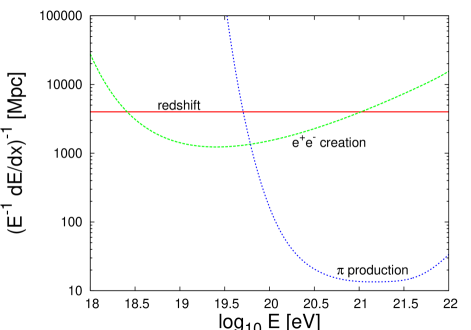
Neutrinos are produced in the decay of the resonance via the channel of charged pion production, see Section 3. The resulting diffuse neutrino flux is usually referred to as the flux of cosmogenic neutrinos or GZK neutrinos. The neutrino flux ranges from approximately eV up to eV. The shape and strength of the neutrino flux depends on various parameters which are described in the next paragraph.
9.1.1 The parameter space
The strength and shape of the cosmogenic neutrino flux depends on seven factors:
-
(i)
the energy spectrum of primary protons - spectral shape, normalization and energy cutoff,
-
(ii)
the proton-photon cross section ,
-
(iii)
the CMB photon density ,
-
(iv)
the evolution of proton-emitting sources with redshift,
-
(v)
the composition of UHECRs,
-
(vi)
magnetic field deflections,
-
(vii)
neutrino oscillations .
Primary spectrum
The spectral shape and normalization of the sources determines the cosmogenic neutrino flux. Typically, it is assumed that all sources follow a powerlaw with an exponential cutoff at a critical energy ,
| (139) |
Such a spectrum can be produced in shock fronts of AGN or GRBs, see Section 3. Monte Carlo simulations indicate a spectral index close to . A generic spectrum with an exact value of is therefore used for all sources in calculations of the cosmogenic neutrino flux. However, it must be noted that recent results from test particle shock acceleration indicate that this value can deviate from depending on the exact shock configuration, see e.g. Bar (04); MBQ07b ; SBS (07). The spectral powerlaw behavior is in accordance with the powerlaw structure of the UHECRs, which are used for the normalization of the total proton spectrum at Earth. This way, no concrete normalization for the single sources needs to be given.
Cross section
Cross section measurements from accelerator data are used in order to estimate the fraction of energy going into neutrinos and the number of neutrinos produced in one interaction. This is done for the complete energy spectrum at the given redshift , and the spectra are propagated from the source to Earth, using a large number of discrete steps of . The value of is chosen to be much smaller than the average mean free path.
CMB photon density
The photon density of the cosmic microwave background, , is well known since its observation with the COBE535353COsmic Background Explorer satellite M+ (90). The spectrum can be fitted with a blackbody spectrum of K,
| (140) |
Evolution of source population with redshift
Typically, it is assumed that ultra high-energy protons are produced in AGN or GRBs, see Section 3. These objects are believed to follow the evolution of star formation and the redshift behavior is often assumed as up to a redshift , with , e.g. Sch (72). At high redshifts, to , the source number counts become small and the exact behavior of for example the distance distribution of AGN is difficult to determine.
Composition of UHECRs
In most neutrino flux predictions, it is assumed that a dominant fraction to the spectrum of UHECRs are protons. While protons are very efficient neutrino generators via interactions, heavier nuclei lose energy via photo-disintegration Ste (69). For instance, iron nuclei interacting with CMB photons induce the following reaction:
| (141) | |||||
| (142) | |||||
| (143) |
In these processes, only very few neutrinos are produced, i.e. via neutron decays. Most models neglect the fraction of heavy nuclei in the spectrum of UHECRs. However, if heavy nuclei dominate the Cosmic Ray spectrum at the highest energies, the neutrino flux can be small as pointed out in HTS (05).
Magnetic field deflections
Protons are deflected by intergalactic magnetic fields and by the magnetic field of the Milky Way on their way to Earth. While this effect could play a role, it is usually neglected in the calculation of cosmogenic neutrino flux predictions. The modelling of extragalactic fields is very difficult, since they are not well-determined.
Neutrino oscillations
Neutrino oscillations are usually not considered in the calculation of the GZK neutrino flux. For a precise determination the changes in the spectrum, oscillation effects would need to be applied after each single propagation effect. However, a good approximation is add up the and spectra at Earth and assume that each of the three flavors are present in equal amounts, as it is the case if the neutrinos are produced far away from Earth.
9.1.2 On the evolution of the GZK neutrino flux model
The existence of the cosmogenic neutrino flux was proposed by Berezinsky & Zatsepin BZ (69) shortly after the prediction of the GZK cutoff was made Gre (66); KZ (68). The first prediction presented in BZ (69) was revised during the years by applying the gained knowledge on the different parameters described above. Table 12 summarizes the development of the model. Each row includes at least one new development in physics or astronomy which was implemented by one or more authors:
-
1969
When the first prediction was made in 1969, the mass of the bosons, , was not yet determined experimentally.
- 1972
- 1985
- 1991
-
2001
The observation of UHECRs above eV lead to the prediction that UHECRs are accelerated up to at least eV. The change in the maximum energy of the primary spectrum also changes the cosmogenic neutrino flux which was pointed out in ESS (01).
-
2005
It was shown in HTS (05) that the cosmogenic neutrino flux is reduced significantly if a large fraction of heavy nuclei is present in the observed flux of UHECRs.
-
2007
It is not clear yet which are the sources of UHECRs. The two primary candidates are AGN and GRBs. These source classes follow different evolution scenarios, which is pointed out in YK (07). GRBs evolve stronger than AGN which leads to an enhanced signal of cosmogenic neutrinos.
| year | ref | evolution | B- | photo- | |||
|---|---|---|---|---|---|---|---|
| dfl. | dis. | ||||||
| 1969 | BZ (69) | unknown | estimate | eV | no | no | no |
| ’72-’75 | e.g. WTW (72), | incl. | estimate | eV | no | no | no |
| Ste (73); BS (75) | |||||||
| ’85-’86 | HS (85), | incl. | CRs | eV | yes | no | no |
| HSW (86) | |||||||
| ’92-’96 | e.g. S+ (91), | yes | impr. | eV | impr. | no | no |
| YT (93); RB (93), | |||||||
| PJ (96) | |||||||
| 2001 | e.g. ESS (01) | yes | CRs | eV | yes | no | no |
| 2005 | HTS (05) | yes | CRs | eV | yes | no | yes |
| 2007 | YK (07) | yes | CRs | eV | impr. | no | no |
In Fig. 28, the energy spectrum of cosmogenic neutrinos is shown for three different models. The uppermost, solid line shows the resulting spectrum if GRBs are responsible for the flux of UHECRs. GRBs are observed to evolve even stronger than different AGN classes, which leads to the enhancement of the flux as shown in YK (07). The current Auger limit comes close to the strong evolution model and with data from the completed Auger array, it will be possible to test this model in detail. The middle, dashed line shows the spectrum for an AGN-type evolution of sources as calculated in RB (93). The lower, dot-dashed line represents the hypothetical spectrum using that UHECRs consist of iron only as calculated in HTS (05); Tay (07) to show that the cosmogenic neutrino flux is decreased significantly with increasing contributions from heavy nuclei in the Cosmic Ray spectrum. It is shown in HTS (05) that, the higher the mass number of the nucleus, the less neutrinos are produced during propagation. A maximum energy of GeV is used for the primary iron nuclei, taking into account the increase of the maximum energy with the charge , see Equ. (12) in Section 3. For lower maximum energies, the flux is further diminished.

9.2 Comparison of event rates in underground detectors
In this section, the expected neutrino rates is calculated for underground detectors in order to get an estimate of the necessary array size for the detection of ultra high-energy neutrinos. Four detector properties have to be considered:
-
1.
The threshold energy of the detector determines the total integral neutrino rate per year and km2. The threshold energy is varied between GeV and GeV in the following calculations.
-
2.
The depth of the detector below the Earth’s surface determines the fraction of neutrinos absorbed before reaching the detector.
-
3.
The effective range of neutrino-induced cascade, . It is determined by the size of the detector, since the cascade has to be induced within the detection array in order to be observed. All following calculations are performed using km. For a constant effective range, the results scale linearly with the range a simple factor can be used to account for different detection array sizes.
-
4.
The density of the detector material, has to be considered as well. The density will be given in terms of , assuming water or ice as the detector medium. For detection arrays in salt, the result can be multiplied by a factor in order to receive the corresponding event rates.
The angle integration was performed over the upper hemisphere () only, since at these energies, no contribution from the lower hemisphere due to absorption. The result is given in units of yr-1 km-3 GeV-1. Three models are compared here,
-
[YK07]
GRB evolution scenario YK (07). With a source evolution matching the one of GRBs, a high neutrino flux is expected. This model is used as the maximum flux possible, since it is close to, but still below, most recent neutrino flux limits.
-
[RB93]
AGN evolution scenario RB (93). The less strong evolution of AGN leads to a reduced neutrino flux compared to the GRB evolution scenario.
-
[HTS05]
Fe iron nuclei as primaries HTS (05); Tay (07). It is assumed that the dominant fraction of Cosmic Rays consists of heavy nuclei. A pure iron spectrum is an absolute lower limit - the neutrino flux increases with the decrease of the mass of the primary nucleus, and it is likely that the spectrum of UHECRs is a composition of light and heavy nuclei. The question of the fraction of heavy nuclei in UHECRs is not answered yet. Therefore, this model is used as a lower limit here.
Since the cross sections for nucleon neutrino interactions do not change significantly with neutrino flavor, the results are basically the same for both flavors. The calculations presented here are performed for electron neutrinos. For muon neutrinos, the results are comparable. In the case of tau-neutrinos, the regeneration of tau leptons needs to be considered as well. Figure 29 shows the integrated electron neutrino detection rates depending on the threshold energy of the detector for the four different GZK neutrino flux predictions. A depth of km is assumed in these calculations. With a detection threshold below GeV, a rate of events/yr/km3 can be expected for the maximum model [YK07]. The AGN evolution model [RB93] yields a factor of less neutrinos and the minimal model using Fe nuclei as primaries results in events/yr/km3. This shows that the instrumentation of volumes significantly larger than km3 is eligible in order to achieve a significant rate of GZK neutrinos per year. This is possible with radio and acoustic detection arrays, since the cascades have a large extension, so that a sparsely instrumented area suffices. Simulations for the extension of IceCube to IceCube Hybrid have been performed, assuming a radio/acoustic array of km2 in the ice around the IceCube detector, together with additional IceCube strings around the original array V+05a . The spacing between the acoustic/radio strings is assumed to be km. While the size of the cascades in the radio and in the acoustic channel is an advantage of these new techniques, the high energy threshold at GeV for radio measurements, and at for acoustic detection of neutrino-induced showers diminishes the rate by up to an order of magnitude as it can be seen from Fig. 29. The total event rate per year is still a few up to 10 events per year for an array of km3 and an AGN evolution scenario.
Table 13 shows how the event rate for electron neutrinos changes with the depth of the detector below the Earth’s surface. Results for five different depths, km, are shown for a threshold energy of GeV. The rate decreases with the depth. It is reduced by a factor of two when the detector is built at km depth instead of km. For threshold energies above GeV as they are expected for radio and acoustic detection, the background of atmospheric muons and neutrinos is negligible. In the case of optical detection, energy cuts can be applied in order to remove lower-energy atmospheric events. Consequently, it is not necessary to deploy the detector deep into the Earth to reduce any background and a detector has the best detection potential at shallow depths of km.

| [kmyr-1] | |||||
|---|---|---|---|---|---|
| [km] | |||||
| YK07 | 1.2 | 0.97 | 0.69 | 0.45 | 0.27 |
| RB93 | 0.44 | 0.34 | 0.25 | 0.17 | 0.10 |
| HTS05 | 0.029 | 0.022 | 0.016 | 0.0010 | 0.0055 |
9.3 Conclusions and outlook
Shortly after the prediction of the GZK cutoff, the first estimates of the cosmogenic neutrino flux were made BZ (69). During the past 40 years, advances in particle physics, e.g. the determination of the mass, as well as in astro- and astroparticle physics, e.g. improving evolution functions, have lead to the improvement of predicted GZK neutrino flux. If UHECRs are protons originating from AGN, an detection rate of about events can be expected in IceCube per year. This event rate is relatively low, since the GZK neutrino flux becomes important at energies above GeV, while the sensitivity of IceCube peaks at lower energies around PeV. Still, the flux should become visible within only a few years of operation due to the extremely low background at these high energies. The event rate for the GZK neutrino flux is expected to be significantly higher with future detection methods, like the acoustic and radio detection. Here, much larger arrays of the order of km3 are planned to be instrumented. For acoustic detection, the lower energy threshold lies at around GeV, for radio detection, it is close to eV. Apart from underground arrays, neutrino-induced electromagnetic and hadronic showers can be detected with balloon experiments, e.g. ANITA, airshower experiments like Auger and Cherenkov telescopes like MAGIC. All these methods have relatively high detection thresholds. Therefore, they are not suited for the observation of point source fluxes from e.g. AGN, but are well-suited for the detection of the diffuse GZK neutrino flux.
Within the next years, it will be possible to further improve the model of the GZK neutrino flux either by the detection of a signal or by setting limits. The sensitivity of a 45 days-flight by ANITA is indicated in Fig. 28. Here, it is already possible to constrict strong evolution models, like those assuming that UHECRs come from GRBs. Together with the detailed examination of the GZK cutoff observed with charged Cosmic Rays by the Auger observatory and other airshower experiments, the search for the GZK neutrino flux will render possible the constraint or the determination of the evolution function of the sources of UHECRs.
10 Summary and conclusions
The concept of multimessenger physics becomes more and more important these days in order to get a complete picture of the sources of investigation. In particular, the non-thermal Universe can only be explained by combining pieces of information from all three messengers, i.e. photons, charged Cosmic Rays and neutrinos. The connection between the observation of charged Cosmic Rays and high-energy photons can only be established by means of high-energy neutrino astrophysics. Hence, the deployment of km3 neutrino detectors is crucial in order to further increase the sensitivity to the flux from extraterrestrial neutrinos.
The modeling of neutrino emission from different sources is essential for the selection of data in large volume neutrino detectors. The different source classes reviewed here, i.e. galactic sources, AGN, GRBs, starbursts and GZK neutrinos, are all analyzed with different methods. These include the search for a diffuse signal at the highest energies, single point source searches, transient source searches and stacking approaches. The different methods help to reduce the background towards the signal expectation.
The fact that neutrino flux limits can be used for physics constraints can be formulated as the Olbers paradox for neutrinos. Olbers pointed out in the 19th century that the fact of a dark night sky contradicted the prevailing theory of the Universe: a homogeneous distribution of stars in an spatially and temporally infinite Universe in thermal equilibrium implied an infinitely bright sky during day and night time. The simple limit of the dark night sky was a first indication that the world view at the time was incomplete. Today, it is known that the Universe is not in thermal equilibrium, which, among other things, leads to the dark night sky. In analogy to this optical limit, the so far dark neutrino sky provides first indications of how to improve current neutrino flux models. The current neutrino flux limits can already be used to restrict different models. In particular, a correlation between X-rays from AGN and neutrinos can be excluded, since models based on this assumption violate recent neutrino flux limits.
Next generation of neutrino telescopes like IceCube and KM3NeT enables a deeper view into the neutrino sky by more than an order of magnitude. With new detection techniques, like the observation of neutrino-induced cascades at radio wavelengths, or the detection of an acoustic cascade in ice or water, enables the investigation of neutrino emission at the highest energies. The combination of different observational techniques renders possible the detailed investigation of a neutrino signal and thereby further advancement in the understanding of multimessenger astrophysics.
Acknowledgments
The outcome of this review article has profited very much from the interaction with different colleagues. In particular, I would like to thank Francis Halzen for intense discussions throughout the years. Many thanks also to Wolfgang Rhode, Peter Biermann, Per-Olof Hulth, Kirsten Münich, Athina Meli, Andrew Taylor, Eli Waxman, Kohta Murase, Lutz Köpke, Andreas Haungs, Justin Vandenbroucke, Christian Spiering, Spencer Klein, Lisa Gerhard, Yolanda Sestayo de la Cerra, Ralf Wischnewski, Jenni Adams, Karl Mannheim, Reinhard Schlickeiser and many more for valuable remarks. Additionally, I would like to thank the IceCube and the MAGIC collaborations for fruitful interactions. Thank you also to the entire astroparticle physics group in Dortmund, for inspiring discussions. Finally, I would like to thank the anonymous referee for very constructive comments and ideas, which helped to improve this review significantly. This work is supported by the Chaudoire award, granted by the Chaudoire foundation, connected to the University of Dortmund.
References
- [1] R. A. Antonov et al. Astropart. Phys., 3:231, 1995.
- [2] K. Asakimori et al. In International Cosmic Ray Conference, page 707, 1995.
- A+ [99] F. Aharonian et al. Phys. Rev. D, 59(9):092003, 1999.
- A+ [01] M. Ave et al. In 27th International Cosmic Ray Conference, page 381, 2001.
- A+ [04] P. Antonioli et al. New J. of Physics, 6:114, 2004.
- A+ [05] T. Antoni et al. Astropart. Phys., 24:1, 2005.
- AA+ [97] J. A. Aguilar, (ANTARES Coll.), et al. astro-ph/9707136, 1997.
- [8] J. Abraham, (Auger Coll.), et al. Science, 318:938, 2007.
- [9] J. Abraham, (Auger Coll.), et al. ArXiv:0712.1909, 2007. submitted to PRL.
- [10] V. Aynutdinov, (Baikal Coll.), et al. Nucl. Instr. & Methods in Phys. Res. A, 567:423, 2006.
- [11] V. Aynutdinov, (Baikal Coll.), et al. Astropart. Phys., 25:140, 2006.
- Aha+ [99] F. A. Aharonian, (HEGRA Coll.), et al. Astron. & Astroph., 349:11, 1999.
- AlH [02] J. Alvarez-Muñiz and F. Halzen. Astroph. J. Lett., 576:L33, 2002.
- [14] F. Aharonian, (HEGRA Coll.), et al. Astron. & Astroph., 403:L1, 2003.
- [15] F. Aharonian, (HEGRA Coll.), et al. Astron. & Astroph., 406:L9, 2003.
- [16] F. Aharonian, (H.E.S.S. Coll.), et al. Astron. & Astroph., 436:L17, 2005.
- [17] F. Aharonian, (H.E.S.S. Coll.), et al. Astron. & Astroph., 442:1, 2005.
- [18] F. Aharonian, (H.E.S.S. Coll.), et al. Science, 314:1424, 2006.
- [19] F. Aharonian, (H.E.S.S. Coll.), et al. Nature, 440:1018, 2006.
- [20] F. Aharonian, (H.E.S.S. Coll.), et al. Astron. & Astroph., 455:461, 2006.
- [21] F. Aharonian, (H.E.S.S. Coll.), et al. Astron. & Astroph., 448:L19, 2006.
- [22] F. Aharonian, (H.E.S.S. Coll.), et al. Astron. & Astroph., 457:899, 2006.
- [23] F. Aharonian, (H.E.S.S. Coll.), et al. Astron. & Astroph., 460:743, 2006.
- [24] F. Aharonian, (H.E.S.S. Coll.), et al. Nature, 439:695, 2006.
- [25] F. Aharonian, (H.E.S.S. Coll.), et al. Astron. & Astroph., 475:L9, 2007.
- [26] F. Aharonian, (H.E.S.S. Coll.), et al. Astron. & Astroph., 470:475, 2007.
- [27] F. Aharonian, (H.E.S.S. Coll), et al. Astron. & Astroph., 473:L25, 2007.
- AI+ [05] A. Achterberg, (IceCube Coll.), et al. IceCube contributions to ICRC 2005, 2005. astro-ph/0509330.
- [29] A. Achterberg, (IceCube Coll.), et al. In J. of Phys., Conference Series, 2006. astro-ph/0611597; http://www.icecube.wisc.edu/tev/.
- [30] A. Achterberg, (IceCube Coll. and P. L. Biermann), et al. Astropart. Phys., 26:282, 2006.
- [31] A. Achterberg, (IceCube Coll.), et al. Astroph. J., 664:397, 2007.
- [32] A. Achterberg, (IceCube Coll.), et al. Phys. Rev. D, 75(10):102001, 2007.
- [33] A. Achterberg, (IceCube Coll.), et al. accepted for publication in ApJ, 2007. arXiv:0705.1186.
- [34] A. Achterberg, (IceCube Coll.), et al. Phys. Rev. D, 76(4):042008, 2007.
- [35] A. Achterberg, (IceCube Coll.), et al. accepted for publication in ApJ, 2007. ArXiv:0711.3022.
- AK+ [04] M. H. Ahn, (K2K Coll.), et al. Phys. Rev. Lett., 93(5):051801, 2004.
- ALS [78] W. I. Axford, E. Leer, and G. Skadron. In 15th International Cosmic Ray Conference, page 132, 1978.
- AM [04] J. Alvarez-Muñiz and P. Mészáros. Phys. Rev. D, 70(12):123001, 2004.
- [39] J. Albert, (MAGIC Coll.), et al. Astroph. J. Lett., 648:L105, 2006.
- [40] J. Albert, (MAGIC Coll.), et al. Astroph. J. Lett., 642:L119, 2006.
- [41] J. Albert, (MAGIC Coll.), et al. Science, 312:1771, 2006.
- [42] J. Albert, , (MAGIC Coll.), et al. Astroph. J. Lett., 666:L17, 2007.
- [43] J. Albert, (MAGIC Coll.), et al. Astroph. J. Lett., 667:L21, 2007.
- [44] J. Albert, (MAGIC Coll.), et al. Astroph. J. Lett., 654:L119, 2007.
- AMR [07] A. de Angelis, O. Mansutti, and M. Roncadelli. ArXiv:0707:4312, 2007. submitted to Phys. ReV. Lett.
- AN+ [05] G. Aggouras, (Nestor Coll.), et al. Astropart. Phys., 23:377, 2005.
- ANT [08] http://antares.in2p3.fr, 2008. ANTARES web-page.
- AS+ [04] S. N. Ahmed, (SNO Coll.), et al. Phys. Rev. Lett., 92(18):181301, 2004.
- Ask [62] G. A. Askaryan. JETP, 14:441, 1962.
- B+ [87] C. Berger et al. Nucl. Instr. & Methods in Phys. Res. A, 262:463, 1987.
- B+ [89] E. V. Bugaev et al. Nuovo Cim. C Geophys. Space Phys. C, 12:41, 1989.
- B+ [93] D. Band et al. Astroph. J., 413:281, 1993.
- B+ [97] G. Boella et al. Astron. & Astroph. Suppl., 122:299, 1997.
- B+ [03] J. F. Beacom et al. Phys. Rev. D, 68(9):093005, 2003.
- B+ [05] S. Böser et al. In Acoustic and Radio EeV Neutrino Detection Activities. World Scientific Publishing, 2005.
- B+ [06] J. K. Becker et al. Astropart. Phys., 25(2):118, 2006.
- [57] J. K. Becker et al. Astropart. Phys., 28(1):98, 2007.
- [58] D. Besson et al. Astropart. Phys., 26:367, 2007.
- BA+ [06] S. W. Barwick, (ANITA Coll.), et al. Phys. Rev. Lett., 96(17):171101, 2006.
- Bar [04] M. G. Baring. Nucl. Phys. B Proc. Suppl., 136:198, 2004.
- Bar [06] S. Barwick. In J. of Phys. - TeV Particle Astrophysics II, Madison, Conference Series, 2006. http://www.icecube.wisc.edu/tev/.
- BAT [08] http://www.batse.msfc.nasa.gov/batse/, 2008. BATSE web-page.
- BBM [05] W. Bednarek, G. F. Burgio, and T. Montaruli. New Astron. Rev., 49:1, 2005.
- [64] J. K. Becker, P. L. Biermann, and W. Rhode. Astropart. Phys., 23:355, 2005.
- [65] J. K. Becker, P. L. Biermann, and W. Rhode. In 29th International Cosmic Ray Conference, 2005.
- Bec [07] J. K. Becker. On the phenomenology of potential astrophysical neutrino sources. PhD thesis, Dortmund University, 2007.
- Bed [05] W. Bednarek. Astroph. J., 631:466, 2005.
- [68] A. R. Bell. Mon. Not. Roy. Astron. Soc., 182:147, 1978.
- [69] A. R. Bell. Mon. Not. Roy. Astron. Soc., 182:443, 1978.
- Bep [08] http://www.asdc.asi.it/bepposax/, 2008. BeppoSax web-page.
- BH [05] W. N. Brandt and G. Hasinger. Ann. Rev. Astron. Astrophys., 43:827, 2005.
- BI+ [05] D. Besson, (IceCube Coll.), et al. In 29th International Cosmic Ray Conference, page 21, 2005.
- Bis [70] G. S. Bisnovatyi-Kogan. Astronomicheskii Zhurnal, 47:813, 1970.
- Bis [71] G. S. Bisnovatyi-Kogan. Soviet Astron., 14:652, 1971.
- [75] J. K. Becker, (MAGIC Coll.), et al. In GRB Conference, Santa Fe, 2007.
- [76] T. Bretz, (MAGIC Coll.), et al. In 30th International Cosmic Ray Conference, 2007.
- BO [78] R. D. Blandford and J. P. Ostriker. Astroph. J. Lett., 221:L29, 1978.
- BO [98] J. Bednarz and M. Ostrowski. Phys. Rev. Lett., 80:3911, 1998.
- Böt [07] M. Böttcher. Astropart. Phys., 27:278, 2007.
- BP [97] W. Bednarek and R. J. Protheroe. Phys. Rev. Lett., 79:2616, 1997.
- BS [75] V. S. Berezinsky and A. Yu. Smirnov. Astrophys. & Space Science, 32:461, 1975.
- BS [87] P. L. Biermann and P. A. Strittmatter. Astroph. J., 322:643, 1987.
- BS [00] P. L. Biermann and G. Sigl. In Lecture Notes in Physics, volume 576, page 1, 2000. astro-ph/0202425.
- BZ [69] V. S. Berezinsky and G. T. Zatsepin. Phys. Rev. Lett., 28(B):423, 1969.
- C+ [89] R. Chini et al. Astron. & Astroph., 221:L3, 1989.
- [86] S. Campana et al. Nature, 442:1008, 2006.
- [87] B. M. Connolly et al. Phys. Rev. D, 74(4):043001, 2006.
- CD [73] T. L. Cline and U. D. Desai. In 11th International Cosmic Ray Conference, page 80, 1973.
- [89] CERN. PDFLIB - User’s Manual, 8.04 edition.
- Chi [06] G. Chincarini. astro-ph/0608414, 2006. to appear in proceedings of Vulcano Workshop 2006.
- CMM [07] A. G. Cocco, G. Mangano, and M. Messina. J. Cosm. and Astr. Phys., 6:15, 2007.
- Con [07] V. Connaughton. In GRB conference, Santa Fe, 2007.
- Cos [01] C. G. S. Costa. Astropart. Phys., 16:193, 2001.
- Cox [72] D. P. Cox. Astroph. J., 178:159, 1972.
- CS [74] D. P. Cox and B. W. Smith. Astroph. J. Lett., 189:L105, 1974.
- CW+ [98] M. Catanese, (Whipple Coll.), et al. Astroph. J., 501:616, 1998.
- D+ [95] K. Daum et al. Zeitschrift für Physik C, 66:417, 1995.
- DA [81] A. M. Dziewonski and D. L. Andersson. Physics of the Earth and Planetary Interiors, 25(4):297, 1981.
- DA+ [06] B. R. Dawson, (Auger Coll.), et al. In J. of Phys. - TeV Particle Astrophysics II, Madison, Conference Series, 2006. http://www.icecube.wisc.edu/tev/.
- Dar [06] A. Dar. Chinese J. of Astron & Astrop. Suppl., 6:301, 2006.
- DCB [99] C. D. Dermer, J. Chiang, and M. Böttcher. Astroph. J., 513:656, 1999.
- DH+ [07] A. Djannati-Ataï, (H.E.S.S. Coll.), et al. In GLAST Symposium, Stanford, 2007.
- DP [90] J. S. Dunlop and J. A. Peacock. Mon. Not. Roy. Astron. Soc., 247:19, 1990.
- DR [04] A. Dar and A. de Rújula. Physics Reports, 405:203, 2004.
- ESS [01] R. Engel, D. Seckel, and T. Stanev. Phys. Rev. D, 64(9):093010, 2001.
- F+ [98] G. Fossati et al. Mon. Not. Roy. Astron. Soc., 299:433, 1998.
- F+ [06] H. Falcke et al. astro-ph/0610652, 2006.
- Fal [96] H. Falcke. In Jets from Stars and Galactic Nuclei, page 19, 1996.
- FB [95] H. Falcke and P. L. Biermann. Astron. & Astroph., 293:665, 1995.
- Fer [49] E. Fermi. Phys. Rev., 75(8):1169, 1949.
- Fer [54] E. Fermi. Astroph. J., 119:1, 1954.
- FMB [95] H. Falcke, M. A. Malkan, and P. L. Biermann. Astron. & Astroph., 298:375, 1995.
- FNV [01] G. Fiorentini, V. A. Naumov, and F. L. Villante. Phys. Lett. B, 510:173, 2001.
- FR [00] E. E. Fenimore and E. Ramirez-Ruiz. astro-ph/0004176, 2000. Report number LA-UR 00-1791.
- FS [96] D. Fargion and A. Salis. In American Institute of Physics Conference Series, page 754, 1996.
- G+ [75] N. L. Grigorov et al. In Cosmic Rays, page 227, 1975.
- G+ [99] M. A. K. Glasmacher et al. Astropart. Phys., 10:291, May 1999.
- [118] P. W. Gorham et al. Phys. Rev. Lett., 93(4):041101, 2004.
- [119] D. Guetta et al. Astropart. Phys., 20:429, 2004.
- G+ [05] P. W. Gorham et al. Phys. Rev. D, 72(2):023002, 2005.
- [121] N. Gehrels et al. Nature, 444:1044, 2006.
- [122] J. Gorosabel et al. Astron. & Astroph., 450:87, 2006.
- GA [03] D. Guetta and E. Amato. Astropart. Phys., 19:403, 2003.
- GA+ [06] P. W. Gorham, (ANITA Coll.), et al. hep-ex/0611008, 2006.
- Gai [90] T. K. Gaisser. Cosmic Rays and Particle Physics. Cambridge University Press, 1990.
- Gai [06] T. Gaisser. In Workshop on Energy Budget in the High Energy Universe, 2006. astro-ph/0608553.
- GHS [95] T. K. Gaisser, F. Halzen, and T. Stanev. Phys. Rep., 258:173, 1995.
- GM [99] N. Gehrels and P. Michelson. Astropart. Phys., 11:277, 1999.
- GM+ [06] J. A. Goodman, (MILAGRO Coll.), et al. In J. of Phys. - TeV Particle Astrophysics II, Madison, Conference Series, 2006. http://www.icecube.wisc.edu/tev/.
- [130] N. Galante, (MAGIC Coll), et al. In GRB conference, Santa Fe, 2007.
- [131] M. Gaug, (MAGIC Coll.), et al. In 30th International Cosmic Ray Conference, 2007.
- GME [93] M. E. Gangl, J. H. Middlestadt, and R. W. Eastes. In Ultraviolet technology IV, San Diego, CA, page 50, 1993.
- Gre [66] K. Greisen. Phys. Rev. Lett., 16, 1966.
- Gro [06] A. Groß. Search for High Energy Neutrinos from Generic AGN classes with AMANDA-II. PhD thesis, Universität Dortmund, 2006.
- GRV [92] M. Glück, E. Reya, and A. Vogt. Z. Phys., C(53), 1992.
- GS [64] V. L. Ginzburg and S. I. Syrovatskii. The Origin of Cosmic Rays. Pergamon Press, 1964.
- GS [03] D. A. Green and F. R. Stephenson. In LNP Vol. 598: Supernovae and Gamma-Ray Bursters, page 7, 2003.
- H+ [92] K. Hurley et al. Astron. & Astroph. Suppl., 92:401, 1992.
- H+ [94] D. H. Hartmann et al. Astroph. J. Suppl. Series, 90:893, 1994.
- H+ [95] M. Honda et al. Phys. Rev. D, 52:4985, 1995.
- H+ [04] M. Honda et al. Phys. Rev. D, 70(4):043008, 2004.
- H+ [05] J. Hjorth et al. Astroph. J. Lett., 630:L117, 2005.
- H+ [06] K. Hurley et al. Astroph. J. Suppl. Series, 164:124, 2006.
- H+ [07] H. He et al. In 30th International Cosmic Ray Conference, 2007.
- Hal [06] F. Halzen. astro-ph/0611915, 2006. proceedings contribution for multimessenger conference in Barcelona (July 2006).
- Hes [12] V. F. Hess. Phys. Z., 13:1084, 1912.
- HET [08] http://space.mit.edu/HETE/, 2008. HETE-II web-page.
- HaH [02] F. Halzen and D. Hooper. Reports of Progress in Physics, 65:1025, 2002.
- Hig [02] High Resolution Fly’s Eye Collaboration. ArXiv: astro-ph/0208301, 2002.
- Hil [84] A. M. Hillas. Ann. Rev. Astron. Astrophys., 22:425, 1984.
- HiR [04] HiRes Coll. Nucl. Phys. B Proc. Suppl., 136:46, 2004.
- HK+ [03] A. Haungs, (KASCADE-Grande Coll.), et al. In 27th International Cosmic Ray Conference, page 985, 2003.
- HKT [07] J. R. Hörandel, N. N. Kalmykov, and A. V. Timokhin. Astropart. Phys., 27:119, 2007.
- HLM [05] F. Halzen, H. Landsman, and T. Montaruli. astro-ph/0503348, 2005.
- HM [84] F. Halzen and A. D. Martin. Quarks and Leptons. Wiley & Sons, Inc., 1984.
- HO [07] F. Halzen and A. O’ Murchadha. arXiv:0705.1723, 705, 2007. XII International Workshop on Neutrino Telescopes, Venice, Italy.
- Hör [03] J. R. Hörandel. Astropart. Phys., 19:193, 2003.
- HS [85] C. T. Hill and D. N. Schramm. Phys. Rev. D, 31:564, 1985.
- HSW [86] C. T. Hill, D. N. Schramm, and T. P. Walker. Phys. Rev. D, 34:1622, 1986.
- HTS [05] D. Hooper, A. Taylor, and S. Sarkar. Astropart. Phys., 23:11, 2005.
- HTS [07] D. Hooper, S. Sarkar and A. Taylor. Astropart. Phys., 27:199, 2007.
- HV+ [01] D. Horan, (VERITAS Coll.), et al. In Gamma 2001: Gamma-Ray Astrophysics, volume 587 of AIP Conference Series, page 324, 2001.
- Jac [06] J. D. Jackson. Klassische Elektrodynamik. de Gruyter, 4th edition, 2006.
- K+ [85] D. D. Krasilnikov et al. In International Cosmic Ray Conference, page 194, 1985.
- K+ [94] G. B. Khristiansen et al. Astropart. Phys., 2:127, 1994.
- K+ [96] S. C. Kappadath et al. Astron. & Astroph. Suppl., 120:C619, 1996.
- K+ [00] J. G. Kirk et al. Astroph. J., 542:235, 2000.
- K+ [01] F. Krennrich et al. Astroph. J. Lett., 560:L45, 2001.
- K+ [03] I. Kravchenko et al. Astropart. Phys., 19:15, 2003.
- K+ [04] H. Krawczynski et al. Astroph. J., 601:151, 2004.
- K+ [07] A. Kappes et al. Astroph. J., 656:870, 2007.
- Kar [62] N. S. Kardashev. Soviet Astron. A. J., 6:317, 1962.
- Kle [04] S. R. Klein. In QCD at Cosmic Energies, Erice (Italy), 2004. astro-ph/0412546.
- KM [07] M. Kowalski and A. Mohr. Astropart. Phys., 27:533, 2007.
- KM [308] see e.g. Proccedings of ”Very Large Volume neutrino Telescopes”, Catania (Italy), Nov 2005, 2008. KM3NeT web-page: http://www.km3net.org/publications.php.
- Koh [13] W. Kohlhörster. Phys. Z., 14:1153, 1913.
- Kon [08] http://heasarc.gsfc.nasa.gov/docs/heasarc/missions/wind.html, 2008. Konus Wind web-page.
- Kos [92] M. Koshiba. Physics Reports, 220:229, 1992.
- KR+ [03] I. Kravchenko, (RICE Coll.), et al. Astropart. Phys., 20:195, 2003.
- KR+ [06] I. Kravchenko, (RICE Coll.), et al. Phys. Rev. D, 73(8):082002, 2006.
- KRB [97] H. Kang, J. Rachen, and P. L. Biermann. Mon. Not. Roy. Astron. Soc., 286(2):257, 1997.
- Kry [77] G. F. Krymskii. Akademiia Nauk SSSR Doklady, 234:1306, 1977.
- KSO [73] R. W. Klebesadel, I. B. Strong, and R. A. Olson. Bullet. American Astron. Soc., 5:322, 1973.
- KW [05] T. Kashti and E. Waxman. Phys. Rev. Lett., 95(18):181101, 2005.
- KW [07] H. B. J. Koers and A. M. J. Wijers. ArXiv:0711.4791, 2007.
- KZ [68] V. A. Kuzmin and G. T. Zatsepin. In 10th International Cosmic Ray Conference, volume 46, page 617, 1968.
- L+ [04] N. G. Lehtinen et al. Phys. Rev. D, 69(1):013008, 2004.
- Lea [79] J. G. Learned. Phys. Rev. D, 19:3293, 1979.
- LP [95] J. G. Learned and S. Pakvasa. Astropart. Phys., 3:267, 1995.
- LUN [08] http://www.physics.adelaide.edu.au/astrophysics/lunaska/index.html, 2008. LUNASKA web-page.
- LW [06] A. Loeb and E. Waxman. J. Cosm. and Astr. Phys., 5:3, 2006.
- M+ [75] E. P. Mazets et al. Astrophys. & Space Science, 33:347, 1975.
- M+ [90] J. C. Mather et al. Astroph. J. Lett., 354:L37, 1990.
- M+ [00] A. Mücke et al. SOPHIA: Monte-Carlo simulations of photohadronic processes. Comput. Phys. Commun., 124:290, 2000.
- [195] P. A. Mazzali et al. Astroph. J. Lett., 599:L95, 2003.
- [196] A. Mücke et al. Astropart. Phys., 18:593, 2003.
- [197] E. P. Mazets et al. Konus catalog of short GRBs. http://www.ioffe.ru/LEA/shortGRBs/Catalog/, 2005.
- [198] S. McGlyn et al. In Gamma-Ray Bursts in the Swift Era, volume 838 of AIP Conference Proceedings, 2005.
- [199] K. Münich et al. In 29th International Cosmic Ray Conference, 2005. astro-ph/0509330.
- M+ [06] K. Murase et al. Astroph. J. Lett., 651:L5, 2006.
- M+ [07] K. Münich et al. In 30th International Cosmic Ray Conference, 2007.
- Mac [98] E. Mach. Über Erscheinungen an fliegenden Projektilen. Separatum ex. Ver. nw. Kenntn., Wien, 1898.
- Man [95] K. Mannheim. Astropart. Phys., 3:295, 1995.
- Mar [08] http://mars.jpl.nasa.gov/odyssey/, 2008. Mars-Odyssey web-page.
- [205] A. Meli, J. K. Becker, and J. J. Quenby. In 30th International Cosmic Ray Conference, 2007. arXiv:0708.1438.
- [206] A. Meli, J. K. Becker, and J. J. Quenby. Cosmic Ray acceleration in subluminal and superluminal, relativistic shock environments. submitted to A&A, 2007.
- Més [06] P. Mészáros. In AIP Conf. Proc. 838: Gamma-Ray Bursts in the Swift Era, page 234, 2006.
- MGI [74] E. P. Mazets, S. V. Golenetskii, and V. N. Il’inskii. volume 19, page 77. JETP Lett., 1974.
- MH+ [07] K. Martens, (HiRes Coll.), et al. In Lepton Photon Conference, 2007. arXiv:0707.4417.
- [210] I. F. Mirabel. astro-ph/0610707, 2006. proceedings contribution for multimessenger conference in Barcelona (July 2006).
- [211] I. F. Mirabel. Science, 312:1759, 2006.
- [212] K. Murase and S. Nagataki. Phys. Rev. D, 73(6):063002, 2006.
- [213] K. Murase and S. Nagataki. Phys. Rev. Lett., 97(5):051101, 2006.
- MOK [06] M. Misiaszek, A. Odrzywołek, and M. Kutschera. Phys. Rev. D, 74(4):043006, 2006.
- Möl [76] C. Möllenhoff. Astron. & Astroph., 50:105, 1976.
- Mon [03] T. Montaruli. In Particle Astrophysics Instrumentation. Proceedings of the SPIE, volume 4858, page 92, 2003.
- MPR [01] K. Mannheim, R. J. Protheroe, and J. P. Rachen. Phys. Rev. D, 63:23003, 2001.
- MR [94] I. F. Mirabel and L. F. Rodriguez. Nature, 371:46, 1994.
- MR [97] P. Mészáros and M. J. Rees. Astroph. J., 476:232, 1997.
- MRS [03] A. D. Martin, M. G. Ryskin, and A. M. Stasto. Acta Phys. Pol. B, 34:3273, 2003.
- MSR [95] K. Mannheim, M. Schulte, and J. Rachen. Astron. & Astroph., 303:L41, 1995.
- Mün [07] K. Münich. Messungen des atmosphärischen Neutrinospektrums mit dem AMANDA-II Detektor - Bestimmung eines 90% oberen Limits auf den extraterrestrischen Beitrag. PhD thesis, Universität Dortmund, 2007.
- Mur [07] K. Murase. Phys. Rev. D, 76:123001, 2007.
- MW [84] E. Mach and J. Wentzel. Anzeiger der Kaiserlichen Akademie der wissensch., Math. Naturw. Classe, Wien, 21:121, 1884. Experimental setup.
- MW [85] E. Mach and J. Wentzel. Kaiserliche Akademie der wissensch., Math. Naturw. Classe, Wien, 92:625, 1885. Experimental results.
- MW [01] P. Mészáros and E. Waxman. Phys. Rev. Lett., 87(17):171102, 2001.
- N+ [06] C. Naumann et al. Int. Journal of Mod. Phys. A, 21:92, 2006.
- NC+ [07] D. Nedbal, (H.E.S.S. Coll.), et al. Astronomical Telegram, 2007. ATEL #1295.
- NEA [08] http://near.jhuapl.edu/instruments/XGRS/, 2008. NEAR web-page.
- NEM [08] http://nemoweb.lns.infn.it/, 2008. NEMO web-page.
- NES [08] http://www.nestor.org.gr/, 2008. NESTOR web-page.
- Nis [99] T. Nishiyama. In 26th International Cosmic Ray Conference, volume 3, page 370, 1999.
- NMB [93] L. Nellen, K. Mannheim, and P. L. Biermann. Phys. Rev. D, 47:5270, 1993.
- NSS [08] http://gammaray.nsstc.nasa.gov, 2008. NSSTC web-page.
- OB [02] M. Ostrowski and J. Bednarz. Astron. & Astroph., 394:1141, 2002.
- Olb [26] H. W. M. Olbers. Über die Durchsichtigkeit des Weltraums. Astron. Jahrb. für das Jahr 1826, 1826. Later puplished in the collection Olbers. Sein Leben und seine Werke, Editor: C. Schilling, Publisher: Julius Springer, Year: 1894.
- OMK [04] A. Odrzywolek, M. Misiaszek, and M. Kutschera. Astropart. Phys., 21:303, 2004.
- OT+ [03] S. Ozawa, (Tibet Asgamma Coll.), et al. In 28th International Cosmic Ray Conference, page 143, 2003.
- P+ [99] W. S. Paciesas et al. Astroph. J. Suppl. Series, 122:465, 1999.
- P+ [02] D. Petry et al. Astroph. J., 580:104, 2002.
- Pal [07] V. Pal’shin. Private Communication, 2007.
- Pir [99] T. Piran. Physics Reports, 314:575, 1999.
- Pir [05] T. Piran. Rev. Mod. Phys., 76:1143, 2005.
- PJ [96] R. J. Protheroe and P. A. Johnson. Astropart. Phys., 4:253, 1996.
- PM [00] R. J. Protheroe and H. Meyer. Phys. Lett. B, 493:1, 2000.
- PM+ [07] E. Prandini, (MAGIC Coll.), et al. In 30th International Cosmic Ray Conference, 2007.
- PRR [95] P. Podsiadlowski, M. J. Rees, and M. Ruderman. Mon. Not. Roy. Astron. Soc., 273:755, 1995.
- PW+ [92] M. Punch, (Whipple Coll.), et al. Nature, 358:477, 1992.
- QW+ [96] J. Quinn, (Whipple Coll.), et al. Astroph. J. Lett., 456:L83, 1996.
- Rac [00] J. P. Rachen. In American Institute of Physics Conference Series, page 41, 2000.
- RB [93] J. P. Rachen and P. L. Biermann. Astron. & Astroph., 272:161, 1993.
- RC [01] W. Rhode and D. Chirkin. In 28th International Cosmic Ray Conference, volume 3, page 1017, 2001.
- RD [96] W. Rhode and K. Daum. Astropart. Phys., 4:217, 1996.
- Ree [70] M. J. Rees. Nature, 227:1303, 1970.
- RHE [08] http://hessi.web.psi.ch/;http://hesperia.gsfc.nasa.gov/hessi/index.html, 2008. RHESSI web-page.
- RI+ [06] E. Resconi, (IceCube Coll.), et al. In J. of Phys. - TeV Particle Astrophysics II, Madison, Conference Series, 2006. astro-ph/0611597; http://www.icecube.wisc.edu/tev/.
- RL [79] G. B. Rybicki and A. P. Lightman. Radiative processes in astrophysics. J. Wiley & Sons, Inc., 1979.
- RM [98] J. P. Rachen and P. Mészáros. Phys. Rev. D, 58(12):123005, 1998.
- RMW [03] S. Razzaque, P. Mészáros, and E. Waxman. Phys. Rev. D, 68(8):083001, 2003.
- Rou [00] E. Roulet. astro-ph/0011570, 2000. Lectures at the ICTP Summer School on Particle Physics and Cosmology.
- S+ [91] F. W. Stecker et al. Phys. Rev. Lett., 66:2697, 1991.
- S+ [01] D. Saltzberg et al. Phys. Rev. Lett., 86:2802, 2001.
- [263] T. Sakamoto et al. Astroph. J., 629:311, 2005.
- [264] M. Schroedter et al. Astroph. J., 634:947, 2005.
- [265] M. Stamatikos et al. In 29th International Cosmic Ray Conference, page 21, 2005. astro-ph/0510336.
- S+ [06] A. Smith et al. In TeV Particle Astrophysics II, 2006. http://icecube.wisc.edu/tev/presentations.php.
- [267] O. Scholten et al. In 30th International Cosmic Ray Conference, 2007.
- [268] D. N. Spergel et al. Astroph. J. Suppl. Series, 170:377, 2007.
- Sak [71] S. Sakashita. Astrophys. & Space Science, 14:431, 1971.
- Sal [06] D. Saltzberg. In J. of Phys. - TeV Particle Astrophysics II, Madison, Conference Series, 2006. http://www.icecube.wisc.edu/tev/.
- Sap [06] P. Sapienza. astro-ph/0611105, 2006. proceedings of the ECRS2006 conference.
- Sat [77] H. Sato. Prog. Theor. Phys., 58(2):549, 1977.
- SBS [07] F. W. Stecker, M. G. Baring, and E. J. Summerlin. Astroph. J. Lett., 667:L29, 2007.
- Sch [63] M. Schmidt. Nature, 197:1040, 1963.
- Sch [72] M. Schmidt. Astroph. J., 176:303, 1972.
- Sch [97] N. Schmitz. Neutrinophysik. Teubner Studienbücher, 1997.
- SdS [92] F. W. Stecker, O. C. de Jager, and M. H. Salamon. Astroph. J. Lett., 390:L49, 1992.
- Sed [58] L. I. Sedov. Rev. Mod. Phys., 30:1077, 1958.
- SMR [05] A. W. Strong, I. V. Moskalenko, and O. Reimer. In AIP Conf. Proc. 745: High Energy Gamma-Ray Astronomy, page 585, 2005.
- StS [96] F. W. Stecker and M. H. Salamon. Space Science Rev., 75:341, 1996.
- SaS [06] T. Sakamoto and Swift-Bat Konus-Wind Hete-II Team. In AIP Conf. Proc. 836: Gamma-Ray Bursts in the Swift Era, page 43, 2006. astro-ph/0605717.
- SSM [05] G. Sinnis, A. Smith, and J. E. McEnery. In 10th Marcel Grossmann Meeting, page 1068, 2005.
- Ste [69] F. W. Stecker. Phys. Rev., 180:1264, 1969.
- Ste [73] F. W. Stecker. Astrophys. & Space Science, 20:47, 1973.
- Ste [05] F. W. Stecker. Phys. Rev. D, 72(10):107301, 2005.
- Ste [07] F. W. Stecker. Astropart. Phys., 26:398, 2007.
- SV+ [07] D. Steele, (VERITAS Coll.), et al. In 30th International Cosmic Ray Conference, 2007.
- Swi [08] http://swift.gsfc.nasa.gov/docs/swift/swiftsc.html, 2008. Swift web-page.
- T+ [06] T. A. Thompson et al. astro-ph/0608699, 2006.
- Tay [07] A. Taylor. Private Communication, 2007.
- TD [07] I. Taboada and M. V. D’Agostino. ArXiv:0711.2277, 2007. submitted to Astroparticle Physics.
- TH [07] D. F. Torres and F. Halzen. Astropart. Phys., 27:500, 2007.
- Uly [08] http://ulysses.jpl.nasa.gov/, 2008. Ulysses web-page.
- V+ [99] H.-H. Voigt et al. Landolt-Börnstein: Numerical Data and Functional Relationships in Science and Technology, 1999.
- [295] J. Vandenbroucke et al. In Acoustic and Radio EeV Neutrino Detection Activities. World Scientific Publishing, 2005.
- [296] G. S. Varner et al. Nucl. Instr. & Methods in Phys. Res. A, 554:437, 2005.
- [297] J. S. Villasenor et al. Nature, 437:855, 2005.
- Van [06] J. Vandenbroucke. In J. of Phys. - TeV Particle Astrophysics II, Madison, Conference Series, 2006. astro-ph/0611503; http://www.icecube.wisc.edu/tev/.
- VB [88] H. J. Voelk and P. L. Biermann. Astroph. J. Lett., 333:L65, 1988.
- VGL [05] J. Vandenbroucke, G. Gratta, and N. Lehtinen. Astroph. J., 621:301, 2005.
- Vie [95] M. Vietri. Astroph. J., 453:883, 1995.
- VM [07] V. Vasileiou and (MILAGRO Coll.). In GRB conference, Santa Fe, 2007.
- Vol [80] L. V. Volkova. Soviet J. of Nuclear Physics, 31:748, 1980.
- W+ [73] W. A. Wheaton et al. Astroph. J. Lett., 185:L57, 1973.
- W+ [01] C. J. Willott et al. Mon. Not. Roy. Astron. Soc., 322:536, 2001.
- Wax [00] E. Waxman. Astroph. J. Suppl. Series, 127:519, 2000.
- WB [97] E. Waxman and J. N. Bahcall. Phys. Rev. Lett., 78:2292, 1997.
- WB [99] E. Waxman and J. N. Bahcall. Phys. Rev. D, 59:23002, 1999.
- WB [00] E. Waxman and J. N. Bahcall. Astroph. J., 541:707, 2000.
- WBM [98] B. Wiebel-Sooth, P. L. Biermann, and H. Meyer. Astron. & Astroph., 330:389, 1998.
- Wei [72] S. Weinberg. Gravitation and Cosmology - principles and applications of the general theory of relativity. John Wiley & Sons, 1972.
- Wei [93] Y. Wei. Untersuchung der neutrinoinduzierten Myonen im Frejus-Untergrunddetektor. PhD thesis, Bergische Universität GH Wuppertal, 1993.
- Win [04] C. Winkler. New Astron. Rev., 48:183, 2004.
- Wis [06] R. Wischnewski. NIM-A, 567:433 2006.
- WKF [98] E. Waxman, S. R. Kulkarni, and D. A. Frail. Astroph. J., 497:288, 1998.
- WL [01] E. Waxman and A. Loeb. Phys. Rev. Lett., 87(7):071101, 2001.
- Wol [72] L. Woltjer. Ann. Rev. Astron. Astrophys., 10:129, 1972.
- WRM [97] R. Wijers, M. J. Rees, and P. Mészáros. Mon. Not. Roy. Astron. Soc., 288:L51, 1997.
- WT [04] P. M. Woods and C. Thompson. astro-ph/0406133, 2004.
- WTW [72] J. Wdowczyk, W. Tkaczyk, and A. W. Wolfendale. J. of Phys. A, 5:1419, 1972.
- [321] S. Yoshida et al. Astropart. Phys., 3:105, 1995.
- [322] S. Yoshida et al. Astropart. Phys., 3:105, 1995.
- YA+ [07] T. Yamamoto, (Auger Coll.), et al. In 30th International Cosmic Ray Conference, 2007. arXiv:0707.2638.
- YK [07] H. Yüksel and M. D. Kistler. Phys. Rev. D, 75(8):083004, 2007.
- You [06] D. S. De Young. Astroph. J., 648:200, 2006.
- YP+ [06] W.-M. Yao, (Particle Data Group), et al. J. of Phys. G, 33:1, 2006.
- YT [93] S. Yoshida and M. Teshima. Prog. Theor. Phys., 89:833, 1993.
- Z+ [07] B. Zhang et al. Astroph. J., 655:989, 2007.
- Zas [05] E. Zas. New J. of Phys., 7:130, 2005.
- ZB [02] C. Zier and P. L. Biermann. Astron. & Astroph., 396:91, 2002.
- ZM [04] B. Zhang and P. Mészáros. Int. J. Mod. Phys. A, 19:2385, 2004.