Sedimentation of pairs of hydrodynamically interacting semiflexible filaments

Abstract

We describe the effect of hydrodynamic interactions in the sedimentation of a pair of inextensible semiflexible filaments under a uniform constant force at low Reynolds numbers. We have analyzed the different regimes and the morphology of such polymers in simple geometries, which allow us to highlight the peculiarities of the interplay between elastic and hydrodynamic stresses. Cooperative and symmetry breaking effects associated to the geometry of the fibers gives rise to characteristic motion which give them distinct properties from rigid and elastic filaments.

I Introduction

The understanding of the hydrodynamics of semiflexible mesoscopic filaments has gained interest due to the relevance of these fibers in different contexts. Many biopolymers are virtually inextensible semiflexible and their dynamics in a fluid plays a central role in the motion of cilia, and eukaryotic and prokaryotic flagella alberts_cell . Although cell motility has been investigated for decades bray , recent advances in microfabrication and micromanipulation enable us to interact directly with them in simplified in vitro environments, where most of the parameters are under control. This allows direct and well defined measurements. For example, Riveline and coworkers riveline have employed optical tweezers to periodically oscillate actin filaments connected to micron-sized beads, in order to devise an artificial “one-armed swimmer”. More recently, Dreyfus et al Dreyfus have been able to produce artificial swimmers out of polymer-linked magnetic beads. This approach enables an easier control of the filaments through magnetic fields, and has allowed to perform quantitative measurements of the physical properties of the chains, such as their bending stiffness, opening a new method to induce properties of the linker molecules gobault or the affinity of the chemical contacts between polymer and particle coating from simple mesoscopic measurements, such as image analysis from video-microscopy koenig . Many other possibilities remain to be explored, ranging from the use of semiflexible filaments in microfluidic devices to the fabrication of synthetic ciliary arrays, or to technological applications of artificial swimmers.

These advances give a renewed stimulus to a quantitative and careful analysis of the hydrodynamics of semiflexible filaments wiggins_bio ; marco2 ; roper ; cebers . They differ from flexible polymers in the ways in which elastic and hydrodynamic stresses compete, and it is necessary to treat both on the same footing, a theoretical challenge. To gain understanding in this interplay and its dynamic implications it is useful to consider the motion of semiflexible chains subject to a uniform external driving. A single sedimenting filament has been considered recently, and it has been shown theoretically marco3 ; xunadim ; Netz_Sed that the chain response differs qualitatively from that of a rigid rod, in accordance with predictions on collective properties of fiber suspensions butler06 . Specifically, the inhomogeneous hydrodynamic stress along the fiber induced by hydrodynamic interactions (HI) leads to filament bending and orientation transverse to the applied field marco3 . Upon increasing the driving, the shape of the filament changes and becomes eventually unstable; the filament then sediments without reaching a steady state.

We will analyze the interactions between a pair of sedimenting filaments, and will study how the combined effect of HI and elasticity induce cooperativity in their motion. The response of the fibers depends on the specific geometry; in particular the translation-rotation coupling is sensitive to the symmetry of the relative positioning of the fibers. Although it is known that translation-rotation couplings lead to an intricate behavior in the sedimentation of rigid rod suspensions butler02 , flexibility leads to new scenarios.

Hence, we will consider three simplified situations. In order to address the role of hydrodynamic cooperativity in the absence of symmetry breaking and induced rotation, we will analyze first two cases where such a coupling is prevented. We are then able to find the relevant scaling regimes for the velocity and the short- and long-time deformation amplitudes, as a function of the inter-filament distance. Subsequently, we will focus in two collinear filaments, the simplest geometry where rotation is induced. The proposed situations can be realized experimentally in a straightforward way, to test our predictions.

The remainder of the paper is organized as follows. In section II we present our computational model, defining the relevant parameters of the system. In section III we summarize the relevant features of single filament sedimentation, which will be useful in subsequent sections. In section IV, we analyze the sedimentation of a pair of semiflexible filaments. We conclude in section V with a discussion of the main results and their implications.

II Model

We study numerically the dynamics of inextensible semiflexible filaments of length $L$, which are characterized by their bending energy. Such an approach is relevant for a large class of biological and non-biological polymers including DNA, cytoskeletal filaments and carbon nanotubes Liverpool , as well as for filaments where the degree of extensibility is negligibly small.

A semiflexible filament can be described by the arclength distance along the filament at a given time $t$, ${\bf r}(s,t)$, where $s\in[0,1]$. Accordingly, its local curvature is $C[{\bf r}(s,t)]=|\partial^{2}{\bf r}(s,t)\ /\partial s^{2}|$, and once the inextensibility constraint is enforced, the elastic energy is given by the Hamiltonian

$${\mathcal{H}}=\frac{1}{2}\kappa\int_{0}^{L}C[{\bf r}(s,t)]^{2}ds\ \ ,$$ (1)

where $\kappa$ stands for the filament’s stiffness.

We model such a filament as a chain of $N$ spheres (“beads”) of radius $a$, connected by bonds of fixed distance $b$. Correspondingly, the bending energy is expressed as the discretization of the Hamiltonian,

$${\mathcal{H}}_{b}=\frac{\kappa}{b}\sum_{i=2}^{N-1}\left(1-\cos\theta_{i}\right)\ \ ,$$ (2)

where $\theta_{i}$ is the angle between the bond that connects bead $i-1$ to bead $i$ with the one that connects bead $i$ with bead $i+1$. The need to resolve the conformational change of the filament makes the simulations computationally much more intensive than when considering rigid rods butler02 . The change in bending energy ${\mathcal{H}}_{b}$ due to the change in position of bead $i$ determines the bending restoring force acting on it, ${\bf F}_{iB}$. Inextensibility implies that the total polymer length is fixed, $L=b(N-1)$; this quantity is kept constant by constraint forces, ${\bf F}_{iC}$, applied at every time step on each bead $i$ marco2 ; Lowe .

It is usual to find biopolymers in suspension. Accordingly, we need to account for the interactions with the embeding solvent. Since the Reynolds numbers are small (in water suspensions, $Re\sim 10^{-6}$ for micron size filaments moving at micrometer per second, and $Re\sim 1$ only for millimeter size filaments displacing at millimeter per second) we need to account for the coupling between elastic and viscous stresses acting on the chains. To this end, we consider that each bead $i$ is subject to a local friction force

$${\bf F}_{iF}=-\gamma_{0}({\bf v}_{i}-{\bf v}_{i}^{H}),$$ (3)

where $\gamma_{0}=6\pi\eta a$ is a friction coefficient related to the bead size and the solvent viscosity, $\eta$, while ${\bf v}_{i}^{H}$ stands for the velocity of the solvent generated by the forces that the rest of the beads exert on the fluid at the position of bead $i$. These dissipative forces couple hydrodynamically all the chain beads through the solvent, giving rise to the hydrodynamic interactions (HI). According to the standard procedure in polymer physics, we describe the flow generated by the filament at the level of the Oseen approximation. Hence, the induced velocity at the position of bead $i$ can be expressed as doi ; marco3

$${\bf v}_{i}^{H}(t)=\frac{3}{4\gamma_{0}}\frac{a}{b}\sum_{j\neq i}\frac{1+{\bf e}_{ij}(t){\bf e}_{ij}(t)}{r_{ij}(t)/b}\cdot{\bf F}_{j}(t),$$ (4)

where $a$ determines the hydrodynamic coupling relevance while ${\bf e}_{ij}=({\bf r}_{i}-{\bf r}_{j})/r_{ij}$ is the unit vector joining beads $i$ and $j$,with $r_{ij}=|{\bf r}_{i}-{\bf r}_{j}|$ being the distance between them; ${\bf F}_{j}$ refers to the total force acting on bead $j$. Although alternative and more accurate approximations to the induced velocities can be implemented brenner , this simple coupling is enough to capture the essentials of HI on elastic filaments, although for small filament separations our prediction will not be in general quantitatively accurate. Following the usual approach in polymer physics, we take $b=2a$, consistent with the Shish-kebab model. The friction coefficient $\gamma_{0}b/a$ provides a means to relate the model parameters to physical units. The local friction force gives rise to an effective filament friction coefficient which depends on filament configuration; therefore, this approach goes beyond resistive force theory brokaw ; wiggins_bio , which regards the solvent as a passive medium that exerts a constant friction coefficient and which does not account for the change in friction with filament configuration.

The description in terms of a local friction force allows to describe the filament’s dynamics using a molecular dynamics approach based on the total force acting on each bead, ${\bf F}_{i}={\bf F}_{iB}+{\bf F}_{iC}+{\bf F}_{iF}+{\bf F}_{ie}+{\bf F}_{ith}$, with ${\bf F}_{ie}$ and ${\bf F}_{ith}$ the external force and the random force which accounts for thermal fluctuations respectively. Multiple filaments can be also analyzed without any further algorithmic complexity. In this paper we will concentrate on filament sedimentation, where ${\bf F}_{ie}\equiv{\bf F}_{e}$ is a constant external force Llopis_jnnf , in situations where the energetic contributions due to the elastic energy dominate and will therefore neglect thermal forces (${\bf F}_{ith}={\bf 0}$). Non-uniform oscilatory external drivings have also been considered within the same approach in the context of filament swimming Lowe ; marco2 ; Llopis_fla ; Llopis_jnnf .

Note that the choice $b=2a$ implies that, as the number of beads increases, the hydrodynamic aspect ratio of the filament, $a/L$, decreases as $1/N$. The basic hydrodynamic coupling we analyze depends only marginally on this choice. A quantitatively more accurate description of the filament finite thickness would require a computationally costly description of the filament morphology, and would not affect qualitatively the results. We have checked that if we change the number of beads , $N$, but keep the mass and length of the filament constant, the results obtained change less than a few percent in the worst case for values ranging between $N=30$ and $N=100$. Moreover, we observe a clear tendency to convergence on increasing $N$ which implies that the trends described subsequently are robust. The results we will describe have been obtained for filaments with $N=30$. We have taken $L=1$ and the filament density $\rho=1$ while the friction coefficient $\gamma_{0}=5$ sets the time scale. The bead mass is then $m_{b}=\pi/2N^{3}$. Numerically, one has to resolve the non-physical inertial time scale in which the bead’s acceleration decays; hence we take the time step $10^{-6}$. The bending rigidity was varied to control the filament flexibility, but the characteristic associated time scale is always larger than the inertial time scale, ensuring that inertia becomes irrelevant at the scales in which the filament configuration evolves.

III Sedimentation of a single semi-flexible filament

We briefly describe the main features of single filament sedimentation, which has been explored both analytically and computationally marco3 ; Netz_Sed ; xunadim , in order to help with the analysis in the coming sections. Filament sedimentation can be described in terms of the dimensionless parameter $B=L^{3}F_{e}/\kappa$, the ratio of the energy imparted by the external force and bending energy marco3 . We disregard thermal effects, which we consider subdominant.

If an external homogeneous force (${\bf F_{e}}$) is applied transversally to the filament axis, its shape reaches a steady state as a result of the competition between elastic, constraint, external and friction forces. Since the friction force acting on beads near the chain’s ends is smaller than the local friction in their center, filaments bend and align perpendicular to the externally applied field. For low to intermediate values of B, chain sedimentation can be characterized by the bending amplitude, $A$, defined as the distance between the highest and lowest beads along the direction of the applied field. For $B<50$, the filament’s amplitude increases linearly; at $B\sim 200$ a plateau is reached, signaling a saturation of the filament deformation in response to the applied field, as depicted in Fig. 1. At even larger values of $B$, metastable shapes with two minima are observed marco3 .

If the chain is not aligned perpendicular to the applied field, the friction force is not balanced and it generates a net torque that will align the filament perpendicular to the external force marco3 ; xunadim . For weak forcings, where the degree of bending is proportional to $B$, the torque generated is also proportional to $B$.

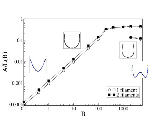
Figure 1: Bending amplitude of a single and a pair of sedimenting filaments, separated a distance $d/L=0.1$, as a function of the dimensionless parameter $B$.

However, the time it takes the polymer to rotate increases as $1/B$ for weak forcings, leading to a singular behavior for a rigid rod ($B=0$), in which the filament keeps its initial orientation because it takes an infinite time to rotate the filament to its perpendicular orientation, a feature that is not captured by resistive force theory. Hence, a single elastic polymer reacts to an applied field in a qualitatively different way than a rigid one.

IV Sedimentation of a pair of flaments

We will now consider pairs of symmetric filaments of length $L$ and rigidity $\kappa$, at a distance $d$ and subject to an external uniform force field ${\bf F}_{e}$. We assume that ${\bf F}_{e}$ is parallel to ${\bf e}_{z}$ and that the polymers lie initially perpendicular to the applied field, along the ${\bf e}_{x}$ direction. The details of the cooperativity induced by the hydrodynamic coupling are sensitive to the initial configuration. To distinguish between different effects induced by hydrodynamics, we will consider three different geometries, as depicted in Fig. 2, which correspond to parallel (geometries I and II), and collinear (geometry III) filaments. Geometries I (Fig. 2.a) and II (Fig. 2.b) preserve the mirror symmetry with respect to the filament’s center while geometry III (Fig. 2.c) will allow us to explore the effects of translation-rotation coupling. We will see that geometry I conserves the symmetries of the one-filament case, and geometry II breaks the up- down symmetry.

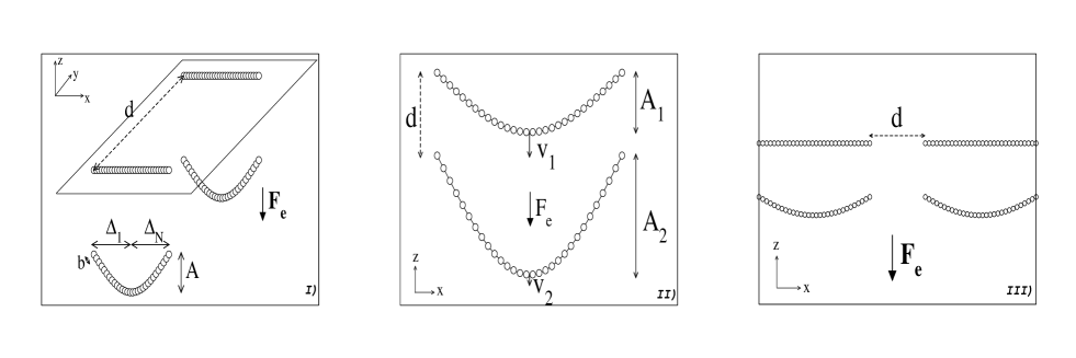
Figure 2: Pairs of semiflexible filaments characterized by their stiffness $\kappa$ and length $L$ that are separated a distance $d$, when they sediment under the action of a uniform external force field, $F_{e}$, for three different geometries; in the three cases we show the relevant parameters. I) Geometry I: Parallel filament sedimenting due to a uniform force transverse to the plane defined by them. II) Geometry II: Sedimenting coplanar filaments. III) Geometry III: Sedimenting collinear filaments

The presence of a second chain modifies the friction exerted on the first filament. As a result, the filament shape and velocity will change as a function of the distance between chains. Depending on their initial conditions, the presence of a second thread can induce rotation of the sedimenting polymer, breaking the mirror symmetry. We will characterize this translation-rotation coupling through the deformation asymetry parameter,

$$D=\frac{\Delta_{1}-\Delta_{N}}{\Delta_{1}+\Delta_{N}}$$ (5)

where $\Delta_{k}=\left|x_{k}-x_{min}\right|$ is the distance along the $x$-direction between the $k$-th bead and the lowest bead, as shown in Fig. 2.a. The parameter $D$ ranges between $[-1,1]$, and reflects the transverse asymmetry of the filament ends. For a single filament, there is no shape asymmetry and $D=0$.

IV.1 Geometry I. Parallel Filaments Under a Force Transverse to the Plane They Define.

The first geometry under consideration involves two filaments that are parallel and transverse to the external force (Fig. 2.a). Due to the initial configuration, they will sediment at the same speed with $D=0$ and keeping their initial separation $d$. After a short time interval, in which HI propagate and the filaments’ inertia decays, they reach their steady state sedimentation velocity and deform into shapes analogous to the ones described for single polymer sedimentation.

Since in our model HI propagate instantaneously, the sedimentation velocity of the initially straight filaments after one time step will deviate from its free draining value $v_{0}\equiv F_{e}/N\gamma_{0}$; in appendix A we compute this initial velocity. Subsequently, the filaments will deform until they reach a new steady state in which they fall down at a different speed. Hence, hydrodynamic cooperativity shows up in the degree of filament bending and its dependence on chains separation.

Bending amplitude.

The filament deformation can be characterized through the same bending amplitude, $A$, defined for single filament sedimentation. For a given value of $B$, $A$ will now depend on filaments’ separation, $d$. We have found that $A(d)$ is consistent with an algebraic decay,

$$A(d)\sim d^{-3}.$$ (6)

as displayed in Fig. 3.a. The dependence of $A$ on $B$ for a pair of filaments separated a distance $d$ does not differ quantitatively from the one observed for a single filament if we compare the filament’s shape with equal values of the parameter $A$. The effect of the second filament can hence be understood in terms of an effective bending energy. Making use of Fig. 1, it is possible to reproduce the filament’s shape by identifying $B_{eff}(d)$ once $A$ has been measured.

Sedimentation velocity.

The presence of a second filament leads to an increase of the sedimentation velocity, which decays algebraically down to small distances,

$$v(d)\sim d^{-1}$$ (7)

as shown in the inset of Fig. 3.b. Such a functional dependence derives from the form of HI at Oseen level Llopis_jnnf . As a result of such coupling, two sedimenting filaments affect each other at large distances, and the coupling becomes quantitatively relevant at distances of the order of the filament’s size.

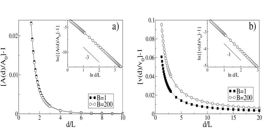
Figure 3: a) Bending amplitude, $A$, and b) velocity in the direction of the force field as a function of filaments’ separation for Geometry I, at $B=1$ and $B=200$. The asymptotic values of $A$ are defined as $A_{0}\equiv A(d\to\infty)$, are $A_{0}(B=1)/L=9.43\times 10^{-4}$ and $A_{0}(B=200)/L=3.40\times 10^{-1}$. Velocities are expressed in units of the sedimentation velocity of an isolated filament, $v_{0}(B)\equiv v(d\to\infty,B)$.

For a given separation $d$, the velocity change due to hydrodynamic cooperativity decreases with $B$. More rigid filaments have a larger filament section exposed to the flow induced by the neighbour filament, leading to a larger relative velocity increase.

IV.2 Geometry II. Sedimenting Coplanar Filaments

We consider next a pair of straight parallel chains separated a distance $d$ under the action of a uniform external field coplanar and transverse to the two filaments, as depicted in Fig. 2.b; the symmetry of the geometry ensures again $D=0$. The upper chain bends less than the lower one, $A_{1}<A_{2}$, and sediments faster because it is subject to a smaller drag due to the solvent counterflow. Similar phenomena have been reported for the sedimentation of other flexible objects, such as drops mangastone ; machu . In Fig. 4 we display the relative sedimentation velocity, $v_{r}\equiv|v_{2z}|-|v_{1z}|$, as a function of a prescribed interfilament distance, $d$. The sedimentation velocity increases with $B$ until the filament deformation reaches the plateau depicted in Fig. 1. The relative velocity vanishes at $B=0$ and for larger values of $B$ increases up to a $10\%$. Accordingly, the sedimentation velocity increases until the plateau regime of the filament deformation is reached, where the time scales for displacement and bending do not differ significantly. Since $v_{r}$ vanishes for $B=0$, the relative velocity can change significantly upon increasing the filaments’ flexibility. Moreover, since the relative velocity is always negative the two filaments will always approach and will eventually collide.

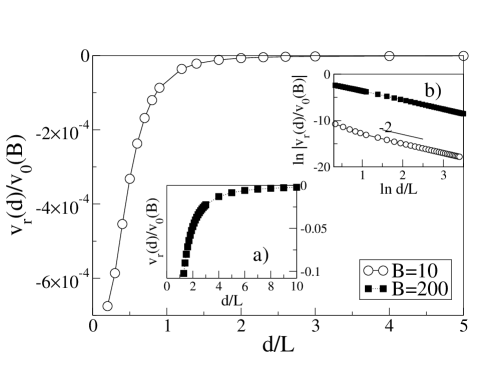
Figure 4: Relative velocity of a pair of initially parallel semiflexible filaments sedimenting on top each other (Geometry II) at $B=10$ normalized by the sedimenting velocity of a single filament at the corresponding $B$, $v_{0}(B)$. a) Relative velocity for $B=200$, where the values of $v_{r}/v_{0}(B)$ are much larger. b) The algebraic dependence of the relative velocity on the distance is compatible with $d^{-2}$.

We have verified that the filaments sedimentation velocity decays as $d^{-1}$, while their relative velocity, $v_{r}$, decays as $d^{-2}$ (Fig. 4) because the leading contribution of $O(d^{-1})$ cancels out exactly. Such a behavior is general and valid for all values of $B$ and in Appendix B we discuss such a dependence on the basis of a simplified limiting model.

IV.3 Geometry III. Collinear Filaments in a Transverse Field

Finally, we analyze the sedimentation of two collinear filaments under the action of a uniform transverse field. To this end, we consider a pair of filaments which are initially straight and with a minimal bead-to-bead distance $d$, as shown in Fig. 2.c.

The hydrodynamic coupling induces a sedimentation velocity which differs from free draining motion, $v_{0}$. Due to the instantaneous propagation of HI in our model, deviatons from $v_{0}$ are observed after one time step. In Appendix oseen_prediction we compute this initial velocity when bending is negligible. The presence of the second filament induces in general a relative displacement of the filaments and also a rotation because the mirror symmetry is lost. The time scales at which filaments rotate and displace depend on filament flexibility.

At short times, when filaments have deformed significantly although their distance has not changed appreciably, one can characterize the filaments by a sedimentation velocity, $v_{s}$, which can be understood as the limit $v_{s}=\lim_{t\to 0}\ v(t)\neq v_{0}$. At long times, filaments approach or move apart and rotate significantly only after they have developed a well-defined bent shape.

In Fig. 5 we show the sedimentation velocity of a pair of filaments at different values of B, as a function of time in units of $\tau_{c}=L\xi_{\perp}/F_{e}$, the time it takes a filament to displace its own size, where $\xi_{\perp}=4\pi\eta L/\log(L/b)$ is the friction coefficient of a rigid rod in the slender body limit. One can see how $v_{s}$ is reached on time scales of order $\tau_{c}$, and that a second, smaller velocity is reached at larger times, when filaments displace and $B$ is not too large. Upon increasing $B$, this second plateau becomes a slow decay toward the long-time regime. The range of this decay also decreases with $B$.

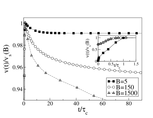
Figure 5: Sedimentation velocity of a pair of filaments at $d/L=0.5$ as a function of time. At $B=5$ the velocity reaches a plateau at small times which is approximately stationary, whereas for $B=150$ the velocity decays after the initial plateau at $t/\tau_{c}\sim 1$. This dependence increases with $B$, as it becomes clear for the curve at $B=1500$. Inset: velocity increase at short times.

In this geometry the long-time sedimentation regime is characterized generically by a coupling between translation and rotation. We will first describe the short-time sedimentation regime, and address the long-time behavior subsequently.

IV.3.1 Short times

The presence of a neighbouring filament induces a deformation that is not symmetric with respect to the center of mass of each filament. The deformation asymmetry increases as the filaments approach, with an algebraic dependence

$$D(d)\sim d^{-2},$$ (8)

as displayed in Fig. 6.a. The change in $D$ arises either because of filament tilt, at small $B$, or due to bending, at large $B$ values.

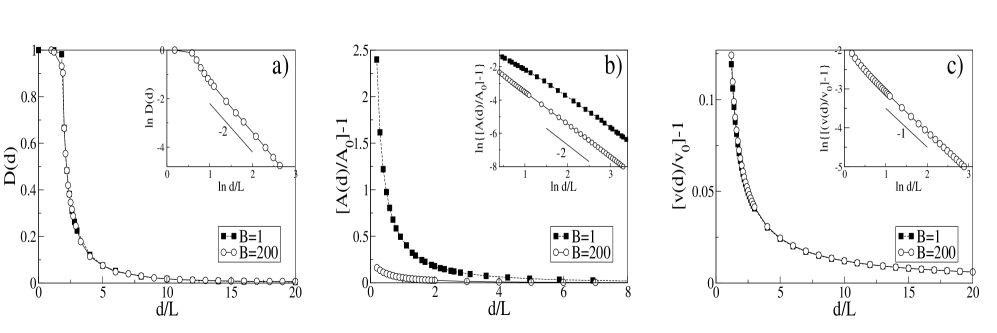
Figure 6: Different measures of the configuration of a pair filaments in the short time regime at $B=1$ and $B=200$ for Geometry III. In all the insets we show the same curves in log-log scale to display their power law dependence which does not depend on $B$. a) Deformation asymmetry, $D(d)$. b) Bending amplitude, $A(d)$, normalized by the corresponding one filament value, $A_{0}$. c) Velocity in the direction of the external force. The asymptotic values are $v_{0}(B=1)=0.52L/\tau_{c}$ and $v_{0}(B=200)=0.50L/\tau_{c}$.

Analogous to the observations in the previous geometries, $A(d)$ decreases algebraically with filament separation, as shown in Fig. 6.b, although with an exponent $-2$ instead of $-3$. The short-time sedimentation velocity $v_{s}(d)$ decays algebraically toward the single filament value algebraically as $1/d$. However, the dependence on $B$ is much weaker than in previous geometries, as displayed in Fig. 6.c. Thus, in the short-time regime we recover practically a universal dependence of the velocity on the distance.

IV.3.2 Long times

In order to analyze the behavior at long times, it is useful to analyze separately the small $B$ ($B<200$)and large $B$ ($B>200$) regimes, corresponding to filaments which do not reach and reach the saturation of single filament deformation, respectively, as shown in Fig. 1).

Small $B$

In this regime, two collinear parallel filaments always tilt, and rotate as a result of the inhomogeneous hydrodynamic stress along every filament. As a result of the rotation and the geometrical asymmetry, we observe a relative velocity, $v_{x}$. In Fig. 7 we display the angular velocity, $\omega$, which shows a crossover from a $d^{-2}$ dependence on filament separation to a weaker $1/\sqrt{d}$ at shorter distances. On the contrary, $v_{x}$ decreases as $1/d$. The weaker dependence at short distances of the angular velocity develops as a result of the translation-rotation coupling; at a fixed distance the angular velocity decays always as $1/d^{2}$. The weaker dependence on filament distance and small magnitude of $\omega$ implies that filaments will usually approach and collide before they have rotated by an angle larger than $\pi/2$, which would allow them to move away from each other (see the example in Fig. 8.a). Only initially remote filaments will avoid collision on observable time scales.

Filament rotation can be clearly analyzed if the initial distance between the two filaments, $d$, is fixed. One can observe that the two filaments rotate with an averaged angular velocity which increases with decreasing $d$, as seen for example in Fig. 8.b. In Appendix C we compute the angular velocity for a pair of paralell sedimenting filaments, which shows the relevance of the translation-rotation coupling.

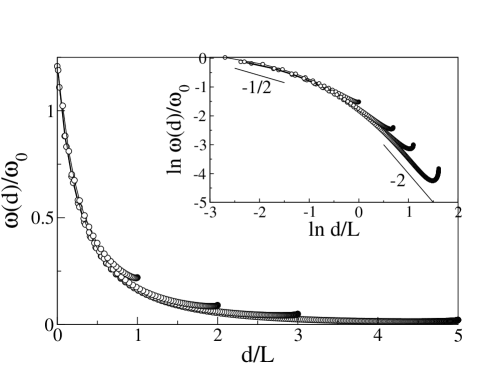
Figure 7: Angular velocity, $\omega(d)$, of a pair of filaments as a function of the distance, for different initial separations, at $B=1$ for Geometry III. $\omega(d)$ is normalized by $\omega_{0}$, the angular velocity at the closest distance. The different curves correspond to different initial separations ($d(t=0)=5,3,2,1$ starting from right to left); after a transient related to the relaxation of the (initially straight) filaments, they follow a unique curve which depends only on the distance betwen the filaments. The inset shows the algebraic behavior at small and large distances.

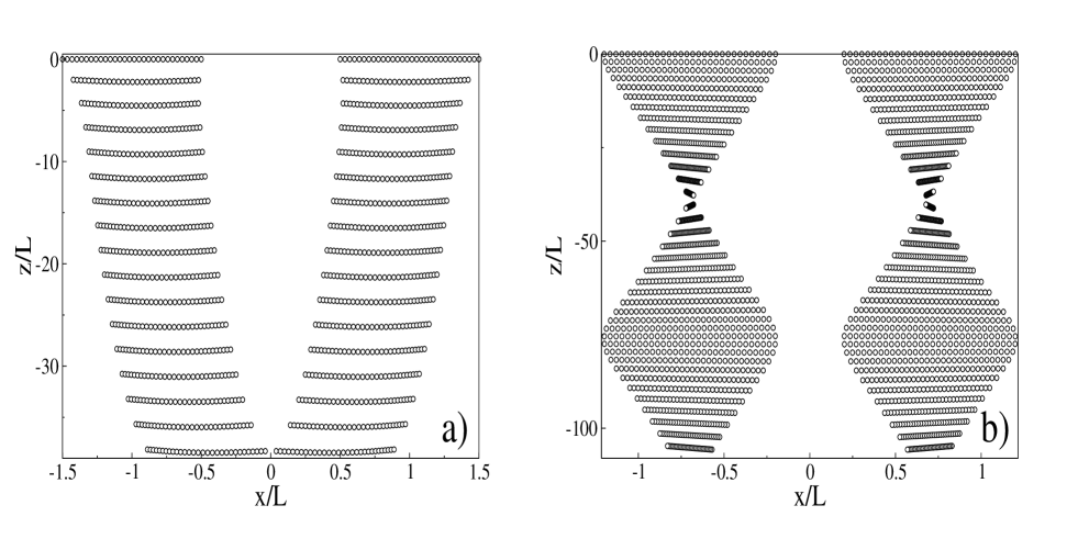
Figure 8: a) Configurations of two initially straight filaments a distance $d/L=1$ away from each other and $B=100$ shown at intervals $t/\tau_{c}=1.2$. At long times ($t/\tau_{c}>>50$) the two filaments eventually collide. b) Configurations of two initially straight filaments a distance $d/L=0.4$ away from each other and $B=1$ shown at intervals $t/\tau_{c}=1.1$. In this case we have fixed $d$ to highlight the rotation of the filaments, characterized by a mean angular velocity which depends on the relative configuration of the two filaments. The apparent shortening of the filament is due to the different scales in the two axis where distances are expressed in units of the filament length $L$.

Large $B$

When the degree of deformation is limited by the length of the filament, its bending is less sensitive to the presence of a second fiber. As a result, the angular velocity that characterizes rotation decreases significantly with B. Associated to this reduced sensitivity, we observe that for any degree of flexibility, at long times there exists a threshold $B^{*}(d)$, such as for $B<B^{*}$ the two filaments approach, while for $B>B^{*}$ move apart after a transient induced by their initial condition, as summarized in the $B-d$ diagram in Fig. 9.a; as $B$ increases filaments move apart at smaller distances. Such a behavior is not present for rigid filaments, and it correlates with the component of the velocity along the filament axis. In Fig. 9.b we show such a velocity as a function of $B$ for a given initial separation, on a time scale in which filaments have displaced distances comparable to their sizes. One can see that the velocity reverses sign at a finite value of $B$, which in fact coincides with the change in behavior displayed in the $B-d$ diagram. When arriving at the bending plateau, for $B>200$, filaments move apart (Fig. 10.a). On the same time scales we have computed the degree of asymmetry $D$, as depicted in Fig. 9.c. The behavior is qualitatively similar to the one observed at short times. As shown in the inset, for very small values of $B$ the filaments essentially only rotate, and only for $B>1$ flexibility starts to affect $D$ quantitatively. Such parameter $D$ also reverses sign at a value of the flexibility similar to that characterizing the change in the velocity. We attribute this change in trend to a crossover from a regime of small $B$, where filaments essentially rotate rigidly, to a regime where the asymmetric deformation is controlled by bending.

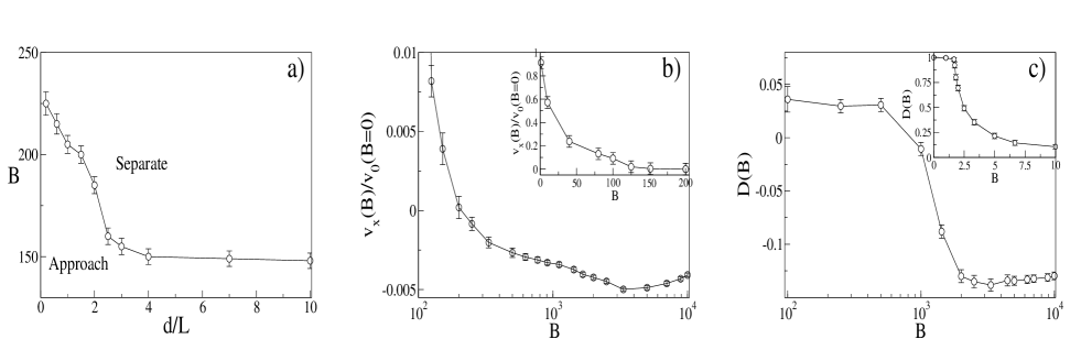
Figure 9: Effective attraction and repulsion in geometry III. a) $B-d$ diagram showing the distinct behaviors of sedimenting collinear filaments as a function of initial distance and driving strength. b) Relative velocity at $t=20\tau_{c}$, when $d=L$, as a function of $B$; positive velocity means attraction. Inset: decay of the relative velocity at small values of $B$. c) Deformation asymmetry at $d=L$ as a function of $B$, showing the change of sign and the minimum value at $B\sim 3000$. Inset: decay at small values of $B$.

At large values of $B$, a third regime is observed both in $v_{x}$ and $D$; both quantities reach a minimum and decrease again in magnitude. The minimum is observed in the parameter region where metastable filament configurations for single filament sedimentation develop. At even larger values of $B$, we have also observed regimes where intrafilament collisions are observed as a result of the shape deformations the filament suffers during its sedimentation. Therefore, the final configuration is not stable and changes continuously with time.

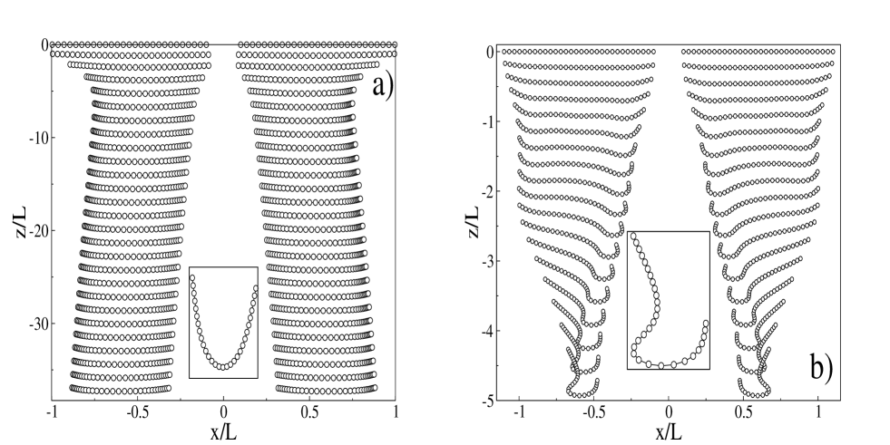
Figure 10: a) Configurations of two initially straight filaments a distance $d/L=0.2$ away from each other and $B=250$ shown at intervals $t/\tau_{c}=2.0$. Filaments repel each other and move apart with a highly curved shape, as shown in the inset for the left fiber. b) Configurations of two initially straight filaments a distance $d/L=0.2$ away from each other and $B=10^{4}$ shown at intervals $t/\tau_{c}=2.3+$. Filaments initially evolve into the metastable configuration described in Fig. 1. while they move apart from each other. During that separation the filaments change their shape and recover transiently this metastable shape. In the inset we show one of the transient, deformed configurations the filaments explore.

V Conclusions

We have studied the sedimentation of a pair of filaments suspended in a low Reynolds number fluid. The coupling that the filaments in the solvent induce on each other through flows, the so called hydrodynamic interactions (HI), give rise to a rich variety of cooperative motion. We have concentrated on the simplest geometries, in order to perform a careful analysis that allow us to focus on the essential features of such cooperativity. To this end, we have implemented and used a simple and efficient numerical method which models the filament as a set of beads and imposes inextensibility where HI are treated at the Oseen approximation.

The geometries we considered have helped us to show that in all cases the sedimentation of a pair of semiflexible filaments is qualitatively different from that of rigid filaments. The rigid limit is in fact singular, and sets in because the time the filaments need to modify their initial configuration increases with filament rigidity, and diverges for infinitely rigid rods. For sufficiently symmetric geometries, such as Geommetry I, HI modify the degree of deformation of each filament and its final sedimentation velocity. The interaction decays algebraically with filament distance, and it becomes quantitatively relevant for separations of the order of the filaments’ size.

For sedimenting parallel coplanar filaments, we have shown that the top filament bends more and moves faster, inducing pair collision, as opposed to the sedimentation of rigid rods.

In less symetric situations, the hydrodynamic coupling induces a rotation and translation of the sedimenting filaments, because their bending lacks the symmetry with respect to the filaments’ center of mass. In these cases, pairs of filaments still interact at long distances, but their sedimentation behavior becomes more involved, and depends on their degree of flexibility as well as their initial conditions. We have shown that such rich behavior includes periodic bound trajectories, filament rotation as well as sedimentation with unsteady conformations.

To sum up, filament flexibility and hidrodynamic coupling modify profoundly the behavior of filament sedimentation; the simplified geometries explored have helped to understand the interplay between elasticity and hydrodynamics and opens the possibilties to analyze in detail how such interactions modify the response of filament suspensions to applied external fields. The study we have carried out has allowed us to make definite predictions that can be tested in controlled experiments, for example with a centrifuge coupled to optical microscopy.

Appendix A Initial sedimentation velocities

In the initial stages of their sedimentation, straight filaments have not deformed significantly. In this regime it is possible to obtain analytical expressions for their sedimentation velocities at the Oseen level.

In particular, we are interested in the velocity that a straight filament oriented along the $x$ direction induces in a second collinear filament a distance $d$ away, as depicted in Fig. 2.c. The external field is applied perpendicular to both filaments, along the $z$ direction, and hence the distance between beads reduces to their separation along the $x$ direction. As a result, the velocity on bead $i$ due to bead $j$ in the direction of the external force, can be expressed as

$$v_{i1}^{H}=\frac{3a}{4}\frac{F_{e}}{\gamma_{0}}\sum_{j}\frac{1}{|x_{j}-x_{i}|},$$ (9)

where we have assumed that bead $i$ belongs to the filament on the left while $j$ is a filament belonging to the filament on the right hand side of the pair, and hence the sum runs over the beads of this second filament. If we approximate the sum by an integral over the length of the filament, we arrive at

$$v_{i1}^{H}=\frac{3a}{4L}\frac{F_{e}}{\gamma_{0}}\int_{L+d}^{2L+d}\frac{\,dx_{j}}{|x_{j}-x_{i}|}=\frac{3a}{4L}\frac{F_{e}}{\gamma_{0}}\ln\left(\frac{2L+d-x_{i}}{L+d-x_{i}}\right).$$ (10)

The contribution of the second filament to the sedimentation velocity of the first one is obtained by computing the induced center of mass velocity. In the continuum approximation, this induced velocity can be written down as $v_{1}^{H}=1/L\int_{0}^{L}v_{i1}^{H}\,dx_{i}$, leading to

$$v_{1}^{H}=\frac{3a}{4L}\frac{F_{e}}{\gamma_{0}}\left\{\frac{d}{L}\ln\left[\frac{d(d+2L)}{(d+L)^{2}}\right]+2\ln\left[\frac{d+2L}{d+L}\right]\right\}.$$ (11)

We can proceed analogously, with obvious modifications in the geometry, to obtain the contribution of a second filament to the sedimentation velocity of the reference one for two coplanar filaments (geometry II). In this case we arrive at

$$v_{1}^{H}=\frac{3a}{4L}\frac{F_{e}}{\gamma_{0}}\left\{2\sqrt{\frac{d^{2}+L^{2}}{L^{2}}}-2\frac{d}{L}+\ln\left[\frac{L+\sqrt{d^{2}+L^{2}}}{-L+\sqrt{d^{2}+L^{2}}}\right]\right\}.$$ (12)

Finally, for Geometry I, if we take the axis of the filaments along the $x$ axis and their distance along the $z$ we get,

$$v_{1}^{H}=\frac{3a}{4L}\frac{F_{e}}{\gamma_{0}}\left\{2\frac{d}{L}-2\sqrt{\frac{d^{2}+L^{2}}{L^{2}}}+\ln\left[\frac{L+\sqrt{d^{2}+L^{2}}}{-L+\sqrt{d^{2}+L^{2}}}\right]\right\}.$$ (13)

In geometries I and II the velocity diverges as the two filaments approach each other because all the beads become infinitely close, as opposed to geometry III which is characterized by a finite induced sedimentation velocity at contact, $3\ln(\sqrt{2})aF_{e}/L\gamma_{0}$.

Appendix B Trimers in Geometry II

In Appendix A, we have computed the initial sedimentation velocity for a pair of filaments where one of them moves on the wake of the neighbouring one (eq. 13). Here we provide an estimate of the rate at which they approach each other when filament deformation is small (either because we focus at short times, or because $B$ is small). We consider the simplest possible case, where the filaments are represented by trimers.

We will calculate the hydrodynamic velocity due to the beads of the neighbor filament on the central beads (depicted in black in Fig 11), defined as $c_{1}$ and $c_{2}$ in Fig 11. The difference between the two velocities is a measure of their relative velocity.

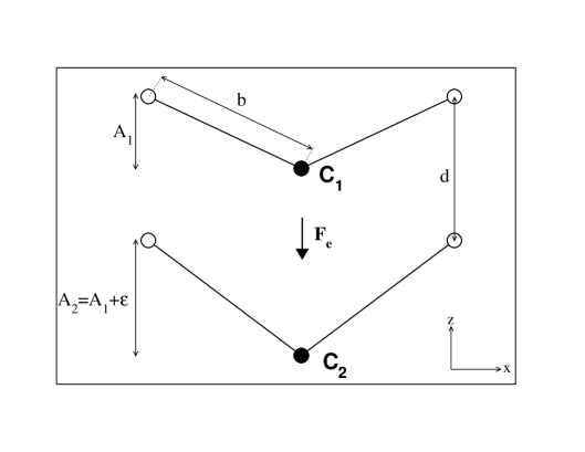
Figure 11: Configuration of a pair of trimers under the action of an external force. The difference on bending amplitude is given by the parameter $\epsilon$.

We characterize $d$ as the distance between the corner beads and the bending amplitude as the separation between the central and corner beads of each filament along the direction of the applied field. The top and bottom chains will bend an amount $A_{1}$ and $A_{2}$ respectively, where $A_{2}\equiv A_{1}+\epsilon$. Hence, $\epsilon$ measures the relative bending amplitude due to the different hydrodynamic coupling. The distance between consecutive beads of a given trimer is $b\equiv L/2$, and the force field has a magnitude $F_{e}$.

The velocity on the central beads $1$ and $2$ has only component in the $z$ direction,

$$v_{c1}=\frac{3a}{2}\frac{F_{e}}{\gamma_{0}}\left\{\frac{2(d-A_{1})^{2}+b^{2}-(A_{1}+\epsilon)^{2}}{\left[(d-A_{1})^{2}+b^{2}-(A_{1}+\epsilon)^{2}\right]^{3/2}}+\frac{1}{d+\epsilon}\right\}$$ (14)

$$v_{c2}=\frac{3a}{2}\frac{F_{e}}{\gamma_{0}}\left\{\frac{2(d+A_{1}+\epsilon)^{2}+b^{2}-A_{1}^{2}}{\left[(d+A_{1}+\epsilon)^{2}+b^{2}-A_{1}^{2}\right]^{3/2}}+\frac{1}{d+\epsilon}\right\}.$$ (15)

Therefore, the relative velocity, $v_{r}\equiv v_{c1}-v_{c2}$, can be expressed as,

$$v_{r} = \frac{3a}{2}\frac{F_{e}}{\gamma_{0}}\left\{\frac{2(d-A_{1})^{2}+b^{2}-(A_{1}+\epsilon)^{2}}{\left[(d-A_{1})^{2}+b^{2}-(A_{1}+\epsilon)^{2}\right]^{3/2}}\right.$$ (16)

$$- \left.\frac{2(d+A_{1}+\epsilon)^{2}+b^{2}-A_{1}^{2}}{\left[(d+A_{1}+\epsilon)^{2}+b^{2}-A_{1}^{2}\right]^{3/2}}\right\}.$$

For small $B$, or large distances, also the differential bending will be small. In this case, if we expand the previous expression in powers of $\epsilon$, we arrive at

$$v_{r}(d,\epsilon)=\frac{3aF_{e}}{\gamma_{0}}\left(2A_{1}+\epsilon+\epsilon^{2}\right)\frac{1}{d^{2}}+O(\epsilon^{3},d^{-4})\ ,$$ (17)

which we have validated using simulations of trimers in this geometry. This expression shows that the top trimer moves faster as a result of HI. The relative velocity depends on the distance as $1/d^{2}$. The increase of $v_{r}$ with $A_{1}$ indicates that also the relative velocity will increase with the flexibility $B$.

Appendix C Rotation of filaments

In section IV.3.2 we have seen that in geometry III, small B filaments rotate and that the parallel filament geometry is unstable. In this appendix we consider a pair of straight filaments, with vanishing bending and constraint forces, oriented along the direction of the external field, $F_{e}$, separated a distance $d$ on the $x$ direction. Hence, we can compute the velocity on each bead due to the presence of the second filament following the same approach as in Appendix A. The components of the velocity on monomer $i$ of a given filament in the directions along and perpendicular to the filaments can be expressed as

$$\left(v_{i}^{H}\right)_{x} = \frac{3a}{4b}\frac{F_{e}}{\gamma_{0}}\sum_{j\neq i}\frac{x_{ij}z_{ij}}{r_{ij}^{3}/b},$$

$$\left(v_{i}^{H}\right)_{z} = \frac{3a}{4b}\frac{F_{e}}{\gamma_{0}}\sum_{j\neq i}\left[\frac{1+(z_{ij}/r_{ij})^{2}}{r_{ij}/b}\right],$$ (18)

where $x_{ij}=|x_{i}-x_{j}|\equiv d$ , $z_{ij}=|z_{i}-z_{j}|$ and $r_{ij}=\sqrt{x_{ij}^{2}+z_{ij}^{2}}$, and where the sums run over the monomers of the same and the neighbouring filaments. Due to the symmetry of the configuration, $(v_{i}^{H})_{x}$ only has nonvanishing contributions from the neighbouring filament, while $(v_{i}^{H})_{z}$ has a contribution for the filament itself, which corresponds to the sedimentation velocity of an isolated filament aligned parallel to the external field, and which in the continuum approximation leads to a sedimentation velocity $(v_{1}^{H})^{\infty}_{z}=F_{e}\ln(L/b)/2\pi\eta L$ in the slender body limit. The contribution of the neighbouring filament increases this velocity to,

$$\left(v_{1}^{H}\right)_{z}=\left(v_{1}^{H}\right)^{\infty}_{z}+\frac{3a}{4L}\frac{F_{e}}{\gamma_{0}}\left[\frac{2}{3d}+\frac{2}{L}\ln(L+\sqrt{d^{2}+L^{2}})\right].$$ (19)

While the filament sediments, it will experience a transverse velocity. Due to the symmetry, this velocity distribution does not lead to any transverse translation; in fact, $(v_{1}^{H})_{x}=(1/L)\sum_{j}(v_{j}^{H})_{x}=0$. This velocity profile yields a net rotation of the filament, which is given, at large distances by $I\omega=m\sum_{ij}z_{ij}(v_{i}^{H})_{x}=(3amF_{e}/4\gamma_{0}L)\left[3/d-7L^{2}/12d^{4}\right]$, where $I=mL^{2}/12$ is the moment of inertia, hence the angular velocity decays asymptotically as $1/d^{2}$, i.e. faster than the approaching velocity $(v_{1}^{H})_{z}$,

$$\omega=\frac{9aF_{e}}{4\gamma_{0}L^{2}}\left[3\frac{1}{d^{2}}-\frac{7L^{2}}{12}\frac{1}{d^{4}}\right].$$ (20)

References

- (1) B. Alberts et al., Molecular Biology of the Cell, Garland Science, New York (2002).
- (2) D. Bray, Cell Movements, Garland, New York (1992).
- (3) D. Riveline, C. H. Wiggins, R.E. Goldstein and A. Ott, Physical Review E 56, R1330 (1997).
- (4) L. Dreyfus, J. Baudry, M. L. Roper, M. Fermigier, H. A. Stone and J. Bibette, Nature 437, 862 (2005).
- (5) C. Goubault, P. Jop, M. Fermigier, J. Baudry, E. Bertrand and J. Bibette, Phys. Rev. Lett. 91, 260802 (2003).
- (6) A. Koenig, P. Hebraud, C. Gosse, R. Dreyfus, J. Baudry, E. Bertrand and J. Bibette, Phys. Rev. Lett. 95, 128301 (2005).
- (7) C.H. Wiggins, D. Riveline, A. Ott and R.E. Goldstein, Biophy. J. 74, 1043 (1998).
- (8) M. C. Lagomarsino, F. Capuani and C.P. Lowe, J. Theor. Biol. 224, 215 (2003).
- (9) M. Roper, R. Dreyfus, J. Baudry, M. Fermigier, J. Bibette and H.A. Stone, Journal of Fluid Mechanics 554, 167 (2006).
- (10) A. Cēbers, Magnetohydrodynamics 41, (2005).
- (11) M. C. Lagomarsino, I. Pagonabarraga and C.P. Lowe, Phys. Rev. Lett. 94, 148104 (2005).
- (12) X. Xu and A. Nadim, Phys. Fluids 6, 2889 (1994).
- (13) X. Schlagberger and R.R. Netz, Europhys. Lett. 70, 129 (2005).
- (14) P.D. Cobb and J.E. Butler, Macromol. 39, 886 (2006).
- (15) J.E. Butler and E.S.G. Shaqfeh, J. Fluid Mech. 468, 205 (2002).
- (16) T. B. Liverpool, Phys. Rev. E 72, 021805 (2005).
- (17) C.P. Lowe, Fut. Gen. Comp. Syst. 17, 853 (2001).
- (18) M. Doi and S. F. Edwards, The Theory of Polymer Dynamics, Oxford University Press, New York (1986).
- (19) M.P. Brenner, Phys. Fluids 11, 754 (1999).
- (20) R.E. Johnson and C.J. Brokaw, Biophys J. 25, (1979).
- (21) I. Llopis, M. C. Lagomarsino and I. Pagonabarraga, submitted.
- (22) I. Llopis, M. C. Lagomarsino, I. Pagonabarraga and C.P. Lowe, in preparation.
- (23) M. Manga and H.A. Stone, J. Fluid Mech. 300, 231 (1995).
- (24) G. Machu, W. Meile, L.C. Nitsche, U. Schaflinger, J. Fluid Mech., 447, 299 (2001).