Hidden in the Light: Magnetically Induced Afterglow from Trapped Chameleon Fields
Abstract
We propose an afterglow phenomenon as a unique trace of chameleon fields in optical experiments. The vacuum interaction of a laser pulse with a magnetic field can lead to a production and subsequent trapping of chameleons in the vacuum chamber, owing to their mass dependence on the ambient matter density. Magnetically induced re-conversion of the trapped chameleons into photons creates an afterglow over macroscopic timescales that can conveniently be searched for by current optical experiments. We show that the chameleon parameter range accessible to available laboratory technology is comparable to scales familiar from astrophysical stellar energy loss arguments. We analyze quantitatively the afterglow properties for various experimental scenarios and discuss the role of potential background and systematic effects. We conclude that afterglow searches represent an ideal tool to aim at the production and detection of cosmologically relevant scalar fields in the laboratory.
pacs:
14.80.-j, 12.20.FvI Introduction
Light scalar fields populate theories of both cosmology and physics beyond the Standard Model. In generic models, these fields can couple to matter and hence potentially mediate a new (or ‘fifth’) force between bodies. However, no such new force has been detected cwill . Any force associated with such light scalar fields must therefore be considerably weaker than gravity over the scales, and under the conditions, that have been experimentally probed. The fields must either interact with matter far more weakly than gravity does, or be sufficiently massive so as to have remained hidden thus far. There is however an assumption when deriving the above conclusions: the mass, , of the scalar field is taken to be a constant. It has recently been shown that the most stringent experimental limits on the properties of light scalar fields can be exponentially relaxed if the scalar field theory in question possesses a chameleon mechanism chamKA ; chamstrong . The chameleon mechanism provides a way to suppress the forces mediated by these scalar fields via non-linear field self-interactions. A direct result of these self-interactions is that the mass of the field is no longer fixed but depends on, amongst other things, the ambient density of matter. The properties of these scalar fields therefore change depending on the environment; it is for this reason that such fields have been dubbed chameleon fields.111This is actually a misnomer: despite popular belief, chameleons (the lizards) cannot change color to their surroundings. Instead, changing color is an expression of their physical and physiological condition wiki:chameleon .. Chameleon fields could potentially also be responsible for the observed late-time acceleration of the Universe chamcos ; chamstruc . In the longer term, it has been shown that future experimental measurements of the Casimir force will be able to detect or rule out many, if not all, of the most interesting chameleon field models for dark energy chamstrong ; chamcas .
It was recently shown that some strongly-coupled (i.e., compared to gravity) chameleon fields would alter light propagation through the vacuum in the presence of a magnetic field in a polarization-dependent manner chamPVLAS ; chamPVLASlong ; the resultant birefringence and dichroism could be detected in laboratory searches such as the polarization experiments PVLAS Zavattini:2005tm ; Zavattini:2007ee , Q&A Chen:2006cd , and BMV Robilliard:2007bq that are sensitive to new hypothetical particles with a light mass and a weak coupling to photons. Popular candidates for these searches are the axion Peccei:1977hh , or more generally an axion-like particle (ALP), minicharged particles (MCPs) Okun:1982xi ; Holdom:1985ag , or paraphotons Okun:1982xi . These particle candidates may be viewed as low-energy effective degrees of freedom of more involved microscopic theories. In this sense, chameleons could be classified as ALPs as far as optical experiments are concerned, but give rise to specific optical signatures to be discussed in detail in this work.
In fact, a variety of further experiments such as ALPS Ehret:2007cm , LIPPS Afanasev:2006cv , OSQAR OSQAR , and GammeV GammeV have been proposed and are currently built up or are even already taking data. They look for anomalous optical signatures from light propagation in a modified quantum vacuum. This rapidly evolving field has been triggered by the fact that optical experiments provide a rather unique laboratory tool, because photons can be manipulated and detected with a great precision. Since laboratory set-ups aim at both production and detection of new particles under fully controlled experimental conditions, they are complementary to astrophysical considerations such as those based on stellar energy loss. The latter can indeed give rather strong bounds, for instance, on axion models Raffelt:2006cw . But for models with particle candidates which exhibit very different properties in the stellar plasma as compared with the laboratory environment, purely laboratory-based experiments are indispensable Masso:2005ym ; chamstrong . The chameleon is exactly of this type, therefore being an ideal particle candidate for high-precision laboratory-based searches.
This work is devoted to an investigation of possible optical signatures which can specifically be attributed to chameleon fields, thereby representing a smoking gun for this particle candidate. The standard optical signatures in polarization experiments are induced ellipticity and rotation for a propagating laser beam interacting with a strong magnetic field Dittrich:2000zu ; these exist for a chameleon chamPVLAS ; chamPVLASlong , but occur similarly for ALPs Maiani:1986md , MCPs Gies:2006ca or models involving also paraphotons Ahlers:2007rd . In the case of a positive signal, the various scenarios can be distinguished from each other by analyzing the signal dependence on the experimental parameters such as magnetic field strength, laser frequency, length of the interaction region Ahlers:2006iz . ALP and paraphoton models can specifically be tested by light-shining-through-walls experiments Sikivie:1983ip ; Ahlers:2007rd ; MCPs can leave a decisive trace in MCP production experiments in the form of a dark current Gies:2006hv .
In this work, we propose an afterglow phenomenon as a unique chameleon trace in an optical experiment.222A similar proposal can be found in DESYgroup . The existence of this afterglow is directly linked with the environment dependence of the chameleon mass parameter. In particular, the mass dependence on the ambient matter density causes the trapping of chameleons inside the vacuum chamber where they have been produced, e.g., by a laser pulse interacting with a strong magnetic field. As detailed below, the trapping can be so efficient that the re-conversion of chameleons into photons in a magnetic field causes an afterglow over macroscopic time scales. Most importantly, our afterglow estimates clearly indicate that the new-physics parameter range accessible to current technology is substantial and can become comparable to scales familiar from astrophysical considerations. Afterglow searches therefore represent a tool to probe physics halfway up to the Planck scale.
This paper is organized as follows: In Sect. II, we review aspects of the chameleon model which are relevant to the optical phenomena discussed in this work. In Sect. III, we solve the equations of motion for the coupled photon-chameleon system, paying particular attention to the boundary conditions which give rise to the afterglow phenomenon. Signatures of the afterglow are exemplified in Sect. IV. The chameleonic afterglow is compared with other background sources and systematic effects in Sect. V. Our conclusions are given in Sect. VI. In the appendix, we discuss another option for afterglow detection based on chameleon resonances in the vacuum chamber.
II Chameleon Theories
As was mentioned above, chameleon theories are essentially scalar field theories with a self-interaction potential and a coupling to matter; they are specified by the action
| (1) | |||||
where is the chameleon field with a self-interaction potential . denotes the matter action and are the matter fields, and we have also explicitly listed the coupling to photons.
The strength of the interaction between and the matter fields is determined by the one or more mass scales . In general, we expect different particle species to couple with different strengths to the chameleon field, i.e., a different for each . Such a differential coupling would lead to violations of the weak equivalence principle (WEP hereafter). It has been shown that can be chosen so that any violations of WEP are too small to have been detected thus far chamstrong . Even though the are generally different for different species, if , we generally expect , with being some mass scale associated with the theory. Provided this is the case, the differential nature of the coupling will have very little effect on our predictions for the experiments considered here. In this paper, we therefore simplify the analysis by assuming a universal coupling .
Note that if the matter fields are non-relativistic. The scalar field, , obeys:
| (2) |
where is the background density of matter. The coupling to matter implies that particle masses in the Einstein frame depend on the value of
| (3) |
where is the bare mass.
We parametrize the strength of the chameleon to matter coupling by where
| (4) |
and . On microscopic scales (and over sufficiently short distances), the chameleon force between two particles is then times the strength of their mutual gravitational attraction.
If the mass, , of is a constant then one must either require that or for such a theory not to have been already ruled out by experimental tests of gravity cwill . If, however, the mass of the scalar field grows with the background density of matter, then a much wider range of scenarios have been shown to be possible chamKA ; chamstrong ; chamcos . In high-density regions, can then be large enough so as to satisfy the constraints coming from tests of gravity. At the same time, the mass of the field can be small enough in low density regions to produce detectable and potentially important alterations to standard physical laws. Assuming as it is above, a scalar field theory possesses a chameleon mechanism if, for some range of , the self-interaction potential, , has the following properties:
| (5) |
where . The evolution of the chameleon field in the presence of ambient matter with density is then determined by the effective potential:
| (6) |
As a result, even though might have a runaway form, the conditions on ensure that the effective potential has a minimum at where
| (7) |
Whether or not the chameleon mechanism is both active and strong enough to evade current experimental constraints depends partially on the details of the theory, i.e. and , and partially on the initial conditions (see Refs. chamKA ; chamstrong ; chamcos for a more detailed discussion). For exponential matter couplings and a potential of the form
| (8) |
the chameleon mechanism can in principle hide the field such that there is no conflict with current laboratory experiments, solar system or cosmological observations chamKA ; chamcos . Importantly, for a large range of values of , the chameleon mechanism is strong enough in such theories to allow even strongly coupled theories with to have remained undetected chamstrong . The first term in corresponds to an effective cosmological constant whilst the second term is a Ratra-Peebles inverse power-law potential ratra . If one assumes that is additionally responsible for late-time acceleration of the universe then one must require .
Throughout the rest of this paper, it is our aim to remain as general as possible and assume as little about the precise form of as is necessary. However, when we come to more detailed discussions and make specific numerical predictions, it will be necessary to choose a particular form for . In these situations, we assume that has the following form:
We do this not because this power-law form of is in any way preferred or to be expected, but merely as it has been the most widely studied in the literature and because is the simplest with which to perform analytical calculations. The power-law form is also useful as an example as it displays, for different values of the , many of the features that we expect to see in more general chameleon theories. We also note how the predictions of a theory with differ from those of a theory with a true power-law potential. With this choice of potential, the constant term in is responsible for the late time acceleration of the Universe.
III Chameleon trapping and photon afterglow
For a chameleon-like scalar field, the classical field equations following from Eq. (1) are
| (9) | |||||
| (10) |
where we have used the Lorenz-gauge condition. We take as the background magnetic field, and as the propagating photon, moving in the positive direction (“to the right”). We perform a Fourier transform with respect to time,
| (11) | |||||
| (12) |
where we have dropped the label , since the photon component parallel to the magnetic field anyway does not interact with the chameleon at all. The notation is introduced here for later convenience. Defining and as the Fourier transforms w.r.t. of and , we arrive at
| (13) | |||||
| (14) |
Solutions exist if
the roots of which define the dispersion relations,
| (15) |
where
| (16) |
Defining , the general solutions and for the equations of motion read:
| (17) | |||||
| (18) | |||||
where is the amplitude of the wave traveling to the left (right). So far, the above equations are very similar to those of a laser interaction with a scalar ALP (or dilaton-like particle) in a magnetic field Maiani:1986md . The important difference between a scalar ALP and a chameleon is due to the boundary conditions at the ends of the optical vacuum chamber: whereas an ALP is considered to be weakly interacting, the chameleon is reflected at the chamber ends and thus “trapped” in the vacuum chamber.
We begin by considering the simplest set-up for an analytic study, wherein the two ends of the vacuum chamber (“jar”) are located right at edge of the magnetic interaction region, i.e., inside the jar and outside. We also confine ourselves to an experiment where the photon field is not stored in an optical cavity as for ALP searches, but simply enters, passes through and leaves the interaction region. The chameleon field is however trapped between two optical windows of the vacuum chamber.
The chameleon field is taken to reflect perfectly off the walls of the jar which are located at and , whereas the photons only enter the jar at and pass straight through. The reflection of the chameleon field implies that at and . This gives
| (19) | |||||
| (20) |
For the photon boundary conditions, it is useful to introduce the operators and which project onto right- and left-moving photon components in vacuum. The condition that no photons enter the jar on the right side at , , gives:
| (21) |
Let as assume that the photon field entering the jar at has the form
| (22) |
with the vacuum dispersion relation . Then, the photon boundary condition at is given by , yielding
| (23) |
Equations (19)-(21) and (23) determine the photon amplitudes completely, and a full solution is straightforward. The physical signature of the chameleon field is encoded in the outgoing photon that leaves the jar at and which we parametrize as
again with the vacuum dispersion . The form of the wave packet as a function of the amplitudes is determined by the matching condition , implying
| (24) |
Since we expect to be a scale beyond the particle-physics standard model, and (1 meV), the dimensionless combination can be considered as a very small parameter for all presently conceivable laboratory field strengths. For typical laboratory laser frequencies , the whole right-hand side of Eq. (16) is small, implying that
| (25) |
is a small expansion parameter for the present problem. We also assume that the laser frequency is larger than the vacuum chameleon mass, , but the combination can still be a sizable number owing to the length of the jar. In these limits, where and , the outgoing wave packet reduces to
| (26) |
Let us study the quotient
We assume that the photon wave packet that is sent into the jar is strongly peaked about . Close to , we then have
Fourier transforming back to real time, the outgoing photon field can be expressed by the functional form of the ingoing photon as:
| (27) | |||||
where , and we have suppressed the dependence which comes in the form of a plane wave . The terms in brackets represent the afterglow effect for the photon mode. Let us assume that for and vanishes otherwise, and define . It is clear that unless the different contributions to the afterglow effect will generally interfere destructively. If and , the afterglow effect will scale as . If then can be of order and so one must ensure that or smaller for the afterglow effect not to be affected by interference. With , this requires to be no greater than a few nanoseconds. The GammeV experiment GammeV uses wide pulses which avoids interference effects. On the other hand, it may be possible to exploit the interference effects for increasing the sensitivity or a determination of the chameleon mass; see the appendix.
Let us generalize the above result to the case, where the jar is longer than the interaction region, as is, for instance, the case for the GammeV experiment GammeV . We let label the beginning of the interaction region. The chameleon reflects off the jar at and . If , the solution to the equation of motions Eqs. (17) and (18) still hold.
Outside the interaction region but inside the jar for , we have:
| (28) | |||||
| (29) |
where and the amplitudes and need to be determined by boundary and matching conditions. In analogy to Eq. (22), we specify the boundary condition of the ingoing wave packet as
| (30) |
where is the vacuum dispersion. Matching the photon amplitudes at the left end of the jar, , where the ingoing wave is purely right-moving, , fixes the amplitude of Eq. (28). Matching the photon amplitudes of Eq. (28) and Eq. (17) at gives
| (31) |
for the right-movers. The corresponding left-mover equation fixes the amplitude of Eq. (28) which contains information about the afterglow effect at the left end of the jar. Here, we concentrate on the afterglow at the right end. For the matching of the chameleon field at , we act with the massive left- and right-moving projectors , on Eqs. (18) and (29), yielding
| (32) | |||
| (33) |
The reflection of the chameleon field at is equivalent to
| (34) |
This replaces Eq. (19) whilst Eqs. (20) and (21) still hold. In conclusion, the matching conditions Eqs. (20),(21) and Eq. (34) (together with Eqs. (32) and (33)) and the boundary condition Eq. (31) completely determine the photon amplitudes . In the limit of small and small , the outgoing wave packet , which is still given by Eq. (24), can be expressed as
| (35) |
Again, for being dominated by the frequency at , the outgoing wave reads
| (36) | |||||
It is important that we mention that by ignoring higher-order terms, we have dropped the information about the decay in the afterglow effect at late times. Since only a finite amount of energy initially converted into chameleon particles for a finite laser pulse, the afterglow effect must eventually decay, the time-scale of which can straightforwardly be estimated: The probability that a chameleon particle converts to a photon as it passes through the interaction region is
| (37) |
After a time , the chameleon field, which had been created by the initial passage of the photons, has moved times back and forth through the interaction region, i.e., from to and then back to again. Since any chameleon particle that is converted into photons escapes, the energy in the chameleon field after time is reduced by a factor
| (38) |
We therefore define the half-life of the afterglow effect by where . Given that , this gives:
We define to be the approximate number of complete passes through the interaction region,
For a realistic estimate of the outgoing wave, we should then replace the infinite upper limit of the sums in Eqs. (27) and (36) by . In the limit , we obtain
We observe that the dependence on the frequency and on the chameleon mass drops out in this limit. For a typical scale and experimental parameters and , we obtain and , corresponding to a time scale that should allow for a high detection efficiency.
IV Signatures of the afterglow
IV.1 General Signatures and Example I: the GammeV set-up
Let us consider the simple case where the pulse length , such that chameleon and photon afterglow propagation inside the cavity happens in well separated bunches. For a pulse, this corresponds to which is, for instance, the case in the GammeV experiment GammeV . As a consequence, there will be no interference between the chameleonic afterglow and the initial pulse. We assume that for , , and before and after this time period. Henceforth, we set .
Then, the afterglow photons also come in bunches of time duration . The th bunch leaves the vacuum chamber to the right at a time in the interval . For and defining , the afterglow amplitude reads:
We identify the modulus of the probability amplitude for an initial photon to reappear in the th afterglow pulse as
| (40) |
Incidentally, this probability amplitude is identical to the chameleon-photon conversion probability stated in Eq. (37), since the pulse-to-afterglow photon conversion involves a photon-chameleon conversion twice. Thus if each pulse contained photons, the number of afterglow photons produced by this pulse after the time with is:
So far, we have neglected the afterglow decay at late times. For larger values of , we must account for the fact that the chameleon amplitude decreases during the photonic afterglow. This is taken care of by the extinction factor of Eq. (38),
| (41) |
For an initial laser pulse with energy and frequency , the number of photons is . A characteristic quantity is given by the detection rate of afterglow photons in the th bunch,
| (42) |
where is the efficiency of the detector. As an example, let us consider the GammeV experiment GammeV with a laser of ns pulse duration, mJ pulse energy and wave length nm. This corresponds to an initial photon rate of . With a magnetic field of and length and assuming that , the early afterglow bunches () arrive at a rate of
In the GammeV experiment GammeV , the half-life, , of the decay of the afterglow effect, in the limit and , is:
| (43) |
The total number of photons contained in the afterglow after a single pulse within the first half-life period is
| (44) | |||||
where we have used the definition of i.e. . In the limit of , the number of afterglow photons in the first half-life period, for instance, for the GammeV GammeV experiment yields
With the conservative assumption of a detector efficiency of , the non-observation of any photon afterglow from one laser pulse in the time would correspond to a lower bound on the coupling scale GeV in the regime of chameleon (vacuum) masses meV. However, to actually achieve such a bound one would have to run the experiment for at least a time of which for GeV is about yrs. It is therefore more practical to consider what lower bound on would result from the non-detection of any photons due to the afterglow of a single laser pulse after a time . We find:
With a minutes worth of measurement, the non-detection of any afterglow from a single pulse of the laser would for meV correspond to a lower bound on the coupling of . If data were collected for a day then this constraint could be raised to .
This should be read side by side with the currently best laboratory bound for similar parameters for weakly coupled scalars or pseudo-scalars derived from the PVLAS experiment Zavattini:2007ee ; from the PVLAS exclusion limits for magnetically-induced rotation at Tesla, we infer GeV.333Similar bounds have also been found by the BMV experiment Robilliard:2007bq and by the earlier BFRT experiment Cameron:1993mr from photon regeneration searches; however, these bounds to not apply to chameleon models, since they involve a passage of the hypothetical particles through a solid wall. We concluded that afterglow experiments are well suited for exploring unknown regions in the parameter space of chameleon models.
As a side remark and a check of the calculation, we note that the total number of photons contained in the full afterglow can be obtained from Eq. (44) by extending the upper bound of the sum to infinity; this yields
which is one half of the total number of photons that would have been initially converted into chameleon particles; the other half creates an afterglow on the other (left) side of the vacuum chamber.
IV.2 Example II: An Optimized Experimental set-up
As a further example, let us consider a more optimized experimental set-up that nevertheless involves only parameters which are achievable by current standard means or systems available in the near future. Our optimized experimental set-up consists of an m long magnetic field of strength T which corresponds exactly to that of the OSQAR experiment at CERN OSQAR . We consider a laser system delivering a sufficiently short pulse with energy kJ and wavelength nm. These parameters agree with the specifications of the laser used by the BMV collaboration Robilliard:2007bq or of the PHELIX laser PHELIX which is currently being built at the GSI (with possible upgrades to several kJ); its designed pulse duration is ns, corresponding to a required chamber length of m. In order to reduce the laser-beam energy deposit on the components of the set-up, the beam diameter may simply be kept comparatively wide (matching the geometry of the detector). Also the pulse duration could be increased while keeping fixed. By increasing the length of the non-magnetized part of the vacuum chamber, the pulse duration can also be extended; e.g., choosing m, the pulse duration could be extended up to 1s without disturbing interference effects. Assuming , The number of afterglow photons in the first half-life period for this optimized set-up (i.e. s, m, T and m) yields
| (45) |
The half-life of the afterglow effect in this set-up is:
| (46) |
Assuming that single photons can be detected in the optimized set-up, , the non-observation of any photon afterglow during from one pulse in would correspond to a lower bound on the coupling scale GeV in the regime of chameleon vacuum masses meV; however for such large values of , the half-life of the afterglow is exceedingly large . It is more reasonable then to ask what lower-bound one could place on if no photons are detected from the afterglow of a single pulse after a time has passed. We find:
| (47) |
We see that after one minute of measurements one could bound , and if measurements could be conducted constantly over a 24 hour period then this could be extended to .
It is interesting to confront these potential afterglow laboratory bounds with typical sensitivity scales obtained from astrophysical arguments: the non-observation of solar axion-like particles by the CAST experiment imposes a bound of GeV for eV Andriamonje:2007ew ; slightly less stringent bounds follow from energy-loss arguments for HB stars Raffelt:2006cw . The similar order of magnitude demonstrates that laboratory measurements of afterglow phenomena can probe scales of new physics that have so far been explored only with astrophysical observations. Of course, we need to stress that these numbers should not literally be compared to each other, since they apply to different theoretical settings; in particular, the astrophysical constraints do not apply to chameleonic ALPs chamPVLAS ; chamPVLASlong , whereas the non-observation of an afterglow would not constrain axion models.
IV.3 Example III: The BMV set-up
As a final example, we consider the recent light-shining-through-a-wall experiment performed by the BMV collaboration Robilliard:2007bq , where a laser with frequency , ns and kJ were used. The magnetic field strength was T, but the magnetic field remained at its maximum values for about ; . If this set-up were modified to search for chameleons trapped in a vacuum chamber then (when ) we would find:
After the chameleons will have made complete passes through the vacuum chamber. If then , and so the duration of the afterglow effect would be limited by the length of the magnetic pulse. For , the total number of afterglow photons produced by each pulse that could potentially be detected in the time interval is (given Robilliard:2007bq ):
We conclude that also the BMV apparatus could search for a coupling parameter beyond GeV. Of course, all experimental set-ups considered here can push the detection limits even further by accumulating statistics.
IV.4 Experimental Bounds on Chameleon Models
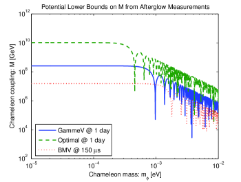
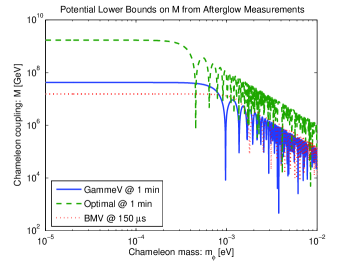
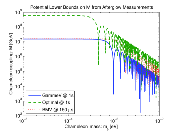
The potential experimental bounds on chameleon models derived from the three examples discussed above are shown in Fig. 1. For the full analysis, we retained the dependence on by taking the full dependence of on into account, cf. Eq. (40). In the case of weak coupling, i.e., large values of , typical values for the half-life of the afterglow are much longer than an experimentally feasible time of measurement. The achievable sensitivity therefore depends on the time duration of the afterglow measurement; for instance, the maximal sensitivity for scales like . In Fig. 1, we show sensitivity bounds for three different measurement durations, s, 1min, 1day.
For small , we rediscover the -independent sensitivity limits which have been discussed analytically in the preceding subsections. For larger , we observe the typical oscillation pattern with sensitivity holes which correspond to full 2 oscillation phases of the photon-chameleon system.
V Background and systematic effects
V.1 Standard Reflection of Photons
So far, we have assumed that the optical windows forming the caps of the jar are completely transparent. In a real experiment, this transparency will be less than perfect and there will be some reflection of photons. For simplicity, we assume that all photons incident on the optical windows are either reflected or transmitted, i.e., we ignore any absorption. We also assume, for simplicity, that the photons hit the optical windows perpendicularly. The coefficients of reflection and transmission are then given by
| (48) |
where and are the indices of refraction for the optical window and the laboratory vacuum, respectively; typical values are and which gives . For the time interval , the rate of afterglow photons leaving the jar at is given by Eq. (42). In this time interval, the photons which have been trapped owing to standard reflection leave the jar at with a rate
where we have neglected a possible interplay between reflection and chameleon trapping; this is justified as long as the time scales for reflection trapping and chameleon trapping are very different. We define by the requirement that for all . We then find that
where we have used , . Even if we still have ; if then . The effect of the standard reflected photons is negligible compared with the afterglow effect for ; moreover, it is clear that generally . For example: with the GammeV parameters ( ns and m), the afterglow dominates after ns if or after about ns if ; both of these time scales are generally far smaller than both the half-life of the afterglow effect and the run-time of the experiments. We conclude that reflection of photons off the caps of the vacuum chamber will not effect the potential of such experiments to detect any chameleonic afterglow.
V.2 Extinction of Chameleon Particles by a Medium
Before we can be sure that the half-life of the chameleon afterglow is, as calculated above, accurate we must consider whether scattering and absorption of chameleon particles by the matter in the laboratory vacuum inside the jar places an important upper limit on the number of passes that the chameleon field makes through the jar. Roughly speaking, if light couples to matter consisting of particles with mass with a strength , then the chameleon field couples to it with a strength . As a beam of light with frequency travels a distance through a medium of free particles with charge , mass and number density , Thompson scattering reduces its intensity by a factor where:
Analogously, the intensity of the beam of chameleon particles traveling within a medium of free particles with mass and number density is reduced by a factor , where
Let us consider for a chameleon field propagating through a laboratory vacuum with pressure . For simplicity, we assume that the vacuum contains only N2 molecules, which gives
After a time , the chameleon particles that were created by the initial laser pulse have traveled on a distance and so scattering has reduced the intensity of the chameleon particles by . We define by , i.e.,
The corresponding half-life due to scattering is thus given by
For , , and , is it clear that
We conclude that the scattering of chameleon particles by atoms in the laboratory vacuum is negligible over the time scales of interest, .
V.3 Quality of the Vacuum
We have found that the mass of the chameleon particles inside the interaction region plays a role in determining the rate of afterglow photon emission. In this rate was found to be
and that the half-life for this effect is:
| (49) |
One of the key properties of chameleon fields is that the mass, , is not fixed but depends on the density environment, which is in turn determined by the quality or pressure, , of the vacuum. From Eq.(49), it is clear that the probability , and hence the afterglow photon rate is greatly suppressed, if . Additionally, if then is almost independent of . The effective local matter density to which the chameleon couples is and only depends on . Thus decreasing can only reduce and hence so far. In all experiments, the smaller vacuum pressure always increases the range of potentials and parameter space than can be detected or ruled out; the downside is that making smaller inevitably increases costs.
Once and are specified, it is always possible to find some value of such that ; we denote the special value of the effective ambient density by . If , then can be realized by setting . Since depends on only through , there is little point in making as opposed to say , as it will increase costs but result in no great chance in the value of . We therefore define the critical value of the vacuum density as so:
The value of is significant as the afterglow rate for is greatly suppressed compared to the rate for . There is also relatively little gain in sensitivity in having as opposed to be . If one is interested in searching for chameleon fields with , where is the smallest value of in which one is interested (e.g. the smallest value of that is not already ruled out by other experiments), the optimal choice for the density of the vacuum, both in terms of experimental sensitively and cost, is .
For definiteness we consider a chameleon theory with power-law potential:
for some and with . The scale of could be seen as ‘natural’ if the chameleon field is additionally responsible for the late time acceleration of the Universe. We use parameters for the GammeV experiment GammeV to provide an example. In this set-up , , T and . The most recent PVLAS results imply that chamPVLAS . Taking , we find that with :
If then in this set-up, for , and if then we have for . For models with a power-law potential, the best trade-off between cost and sensitivity for GammeV set-up, would therefore be to use . This corresponds to an optimal vacuum pressure: . A vacuum of this quality was used in the recent PVLAS axion search Zavattini:2005tm ; Zavattini:2007ee . If one could rule out theories with by some other means then very little would be gained in terms of sensitivity to models with by making the vacuum pressure much smaller than: .
If we consider instead the “optimal set-up” that we described in Section IV, then for and , the optimal choice for the vacuum pressure is . In the context of chameleon models with a power-law potential with and , relatively little would be gained in terms of sensitivity by lowering further than this. However, lower values of would increase the ranges of values of and that could be detected.
Notice that, since one can vary the chameleon mass, , by changing the local density, , it would in principle be possible to measure using these experiments as a function of by making use of the relation . One would then know as a function of and hence also up to a constant. From this one could reconstruct . By integrating, one would then arrive at , for some range of . However, since the minimum size of is limited by for , one cannot probe in the region that is cosmologically interesting today, i.e. . It must be stressed though that the sensitivity of ALP experiments to is strongly peaked about values for which , and so it is not the most ideal probe of ; ALP experiments are best suited to measuring or placing lower-bounds on . Casimir force measurements has recently be shown in Ref. chamcas to provide a potentially much more direct probe of but conversely say little about the chameleon to matter coupling, .
VI Conclusions
In this paper, we have investigated the possibility of using an afterglow phenomenon as a unique chameleon trace in optical experiments. The existence of this afterglow is directly linked with the environment dependence of the chameleon mass parameter. The latter causes the trapping of chameleons inside the vacuum chamber where they have been produced, e.g., by a laser pulse interacting with a strong magnetic field. The afterglow itself is linearly polarized perpendicularly to the magnetic field.
We find that the trapping can be so efficient that the re-conversion of chameleons into photons in a magnetic field causes an afterglow over macroscopic time scales. For instance, for values of the inverse chameleon-photon coupling slightly above the current detection limit GeV Zavattini:2007ee and magnetic fields of a few Tesla and few meters long, the half-life of the afterglow is on the order of minutes. Current experiments such as ALPS, BMV, GammeV and OSQAR can improve the current limit on by a few orders of magnitude. With present-day technology, even a parameter range of chameleon-photon couplings appears accessible which is comparable in magnitude, e.g., to bounds on the axion-photon coupling derived from astrophysical considerations, i.e., GeV.
In the present work, we mainly considered the afterglow from an initial short laser pulse, the associated length of which fits into the optical path length within the vacuum chamber. From a technical viewpoint, this choice avoids unwanted interference effects, but it also has an experimental advantage: the resulting afterglow photons all arrive in pulses of the same duration as the initial pulse and are separated by a known time (i.e., ). This can be useful in extracting the signal from any background noise which should not be correlated in this way. Also the polarization dependence of the afterglow can be used to distinguish a possible signal from noise.
As discussed in the appendix, also long laser pulses or continuous laser light could be used in an experiment, if the resulting interference can be controlled to some extent such that a chameleon-photon resonance exists at least in some part of the apparatus. This resonance phenomenon is particularly sensitive to smaller chameleon masses. Unfortunately, a full control of the chameleon resonance may experimentally be very difficult; but if it were possible, the gain in afterglow photons, and subsequently in sensitivity to a chameleonic sector, could be very significant.
We would like to stress again that the afterglow phenomenon in the experiments considered here is a smoking gun for a chameleonic particle. From the viewpoint of optical experiments, a number of further mechanisms have been proposed that could induce optical signatures in laboratory experiments, but still evade astrophysical constraints Masso:2006gc ; Mohapatra:2006pv ; Jain:2006ki ; Foot:2007cq . Distinguishing between the various scenarios in the case of a positive signal for, say, ellipticity and dichroism, may not always be possible with the current laboratory set-ups. But the observation of an afterglow would strongly point to a chameleon mechanism.
In this sense, it appears worthwhile to reconsider other concepts on using optical signatures to deduce information about the underlying particle-physics content, e.g., using strong laser fields Heinzl:2006xc ; DiPiazza:2006pr ; Marklund:2006my or astronomical observations Dupays:2005xs ; tomi1 ; tomi2 ; Mirizzi:2007hr ; DeAngelis:2007yu , in the light of a chameleon field.
Finally, it is interesting to notice that it could, in principle, be possible to measure the varying chameleon mass by varying the vacuum pressure in the experiment and thereby extract information about the scalar potential . The reconstruction of from this afterglow experiment assumes however that the value of that one detects from afterglow experiments (i.e, the photon-chameleon coupling) is the same as the matter-chameleon coupling. This, of course, need not be the case; although we might expect them to be of the same magnitude. By contrast, the reconstruction of from the Casimir force tests chamcas does not run into this problem, since these experiments would effectively measure directly and provide only weak constraints on . If chameleon fields were to be detected, one could, by comparing the reconstructions of from afterglow and Casimir experiments, actually measure not only the chameleon-photon coupling but also the chameleon-matter coupling.
In resume, our afterglow estimates clearly indicate that the new-physics parameter range accessible even with current technology is substantial. Afterglow searches therefore represent a powerful tool to probe physics halfway up to the Planck scale.
Acknowledgements.
We thank P. Brax and C. van de Bruck for useful discussions. HG acknowledges support by the DFG under contract Gi 328/1-4 (Emmy-Noether program). DFM is supported by the Alexander von Humboldt Foundation. DJS is supported by STFC.Appendix A Interference effects
In this appendix, we discuss the possible use of interference effects for the afterglow phenomenon. Whereas the short-pulse experiments considered in the main text provide for a clean signal, the occurrence of interference depends more strongly on the details and the precision of the experiment.
Let us consider a long pulse of duration with frequency and a Gaußian envelope,
| (50) |
In this case, the afterglow amplitude in Eq. (27) or Eq. (36) for a given time at position (say, at a time after the initial pulse has passed the detector at ) receives contributions from many terms in the sum; typically, the Gaußian profile picks up a wide range of large values.
Extending the summation range of from to (instead of to ) introduces only an exponentially small error owing to the Gaußian envelope, but allows to perform a Poisson resummation of the sum; for instance, the term in the second line of Eq. (36) yields ()
| (51) |
where , and we have dropped terms of order and . The Gaußian factor in the last term causes a strong exponential suppression, since and by assumption, and typically . Therefore, this factor essentially picks out one term in the sum that comes closest to the resonance condition
| (52) |
Let us denote the integer that is closest to this resonance condition with . Then the afterglow amplitude reads
| (53) |
where summarizes all phases of the amplitude. Whether or not the resonance condition can be met is a delicate experimental issue. The above formula suggests that the experimental parameters require an extraordinary fine-tuning, since the width of the resonance is extremely small. However, in a real experiment, systematic uncertainties may invalidate the idealized scenario from the very beginning; for instance, the laser beam has a finite cross section, and the length of the vacuum chamber may vary across this cross section a little bit. Variations on the order of the laser wave length lead to uncertainties of order 1 on the right-hand side of Eq. (52). Therefore, the resonance condition might be satisfied for some part of the beam only.
For a simplified estimate, let us assume that the beam cross section is a circular disc. The center of the disc is assumed to satisfy the resonance condition exactly, but the length varies linearly from the center to the edge of the disc by a bit less than half a laser wavelength . Averaging over the Gaußian resonance factor in Eq. (53) then corresponds to integrating radially over the resonance peak. This procedure leads to the replacement
| (54) |
(More resonance points in the beam cross section would give a sum of similar terms on the right-hand side of Eq. (54).) In this case, we can read off the probability amplitude for a photon in the Gaußian pulse to reappear in the afterglow at time averaged over the resonance,
| (55) | |||||
where we have approximated the by its phase average , since the phase is large and may also vary spatially or over the measurement period.
Let us compare the resulting probability for a long pulse s with that of a short-pulse set-up for T, m, nm) in the region of small masses meV,
| (56) |
Here it is important to stress that the calculation has been performed in the limit , corresponding to
| (57) |
In other words, the validity range of Eqs. (55) and (56) does not extend to arbitrarily small masses. Still, for small chameleon masses and larger values of (such that Eq. (57) holds), the averaged resonance probability can exceed that of the short-pulse case in the present example.
Using, for instance, a 10s long pulse from a 100Watt laser, the number of photons in the afterglow will be
| (58) |
where denotes the measurement time of the afterglow. We conclude that such an experiment can become sensitive to the coupling scales of order GeV for chameleon masses in the sub eV range. We stress again that the precise sensitivity limits strongly depend on the experimental details and the feasibility to exploit a chameleon resonance in the vacuum cavity. If such a resonance can be created in an experiment the interference measurement can provide for a handle on a measurement of the chameleon mass, since the dependence on the latter is rather strong.
If a fully controlled resonance could be built up in an experiment, the suppression factor on the right-hand side of Eq. (54) arising from averaging would be replaced by 1; this would correspond to an enhancement factor of for the probability amplitude in the example given above. From an experimental viewpoint, controlling the resonance a priori seems, of course, rather difficult. From the non-observation of an afterglow in a long-pulse experiment, it would be difficult to conclude whether this points to rather strong bounds on or to the fact that the resonance condition is not sufficiently met. We therefore recommend short-pulse experiments as a much cleaner and well controllable set-up.
References
- (1) For a review of experimental tests of the Equivalence Principle and General Relativity , see C.M. Will, Theory and Experiment in Gravitational Physics, 2nd Ed., (Basic Books/Perseus Group, New York, 1993); C.M. Will, Living Rev. Rel. 9, 3 (2006).
- (2) J. Khoury and A. Weltman, Phys. Rev. Lett. 93, 171104 (2004); Phys. Rev. D 69, 044026 (2004).
- (3) D. F. Mota and D. J. Shaw, Phys. Rev. D.75, 063501 (2007); Phys. Rev. Lett. 97 (2006) 151102.
- (4) See, for instance, http://en.wikipedia.org/wiki/Chameleon.
- (5) Ph. Brax, C. van de Bruck, A.-C. Davis, J. Khoury and A. Weltman, Phys. Rev. D 70, 123518 (2004).
- (6) Ph. Brax, C. van de Bruck, A. C. Davis and A. M. Green, Phys. Lett. B 633, 441 (2006).
- (7) P. Brax, C. van de Bruck, A. C. Davis, D. F. Mota and D. J. Shaw, arXiv:0709.2075 [hep-ph].
- (8) Ph. Brax, C. van de Bruck, A. C. Davis, [arXiv:hep-ph/0703243]
- (9) P. Brax, C. van de Bruck, A. C. Davis, D. F. Mota and D. J. Shaw, arXiv:0707.2801 [hep-ph].
- (10) E. Zavattini et al. [PVLAS Collaboration], Phys. Rev. Lett. 96, 110406 (2006) [arXiv:hep-ex/0507107];
- (11) E. Zavattini et al. [PVLAS Collaboration], arXiv:0706.3419 [hep-ex].
- (12) S. J. Chen, H. H. Mei and W. T. Ni [Q& A Collaboration], hep-ex/0611050.
- (13) C. Robilliard, R. Battesti, M. Fouche, J. Mauchain, A. M. Sautivet, F. Amiranoff and C. Rizzo, arXiv:0707.1296 [hep-ex].
- (14) R. D. Peccei and H. R. Quinn, Phys. Rev. Lett. 38, 1440 (1977); Phys. Rev. D 16, 1791 (1977); S. Weinberg, Phys. Rev. Lett. 40, 223 (1978); F. Wilczek, Phys. Rev. Lett. 40, 279 (1978).
- (15) L. B. Okun, Sov. Phys. JETP 56, 502 (1982);
- (16) B. Holdom, Phys. Lett. B 166 (1986) 196.
- (17) K. Ehret et al., arXiv:hep-ex/0702023.
- (18) A. V. Afanasev, O. K. Baker and K. W. McFarlane, arXiv:hep-ph/0605250.
- (19) P. Pugnat et al., CERN-SPSC-2006-035; see http://graybook.cern.ch/programmes/experiments/OSQAR.html.
- (20) see http://gammev.fnal.gov/.
- (21) G. G. Raffelt, arXiv:hep-ph/0611350.
- (22) E. Masso and J. Redondo, JCAP 0509, 015 (2005) [arXiv:hep-ph/0504202]; J. Jaeckel, E. Masso, J. Redondo, A. Ringwald and F. Takahashi, Phys. Rev. D 75, 013004 (2007) [arXiv:hep-ph/0610203].
- (23) for a review, see W. Dittrich and H. Gies, Springer Tracts Mod. Phys. 166, 1 (2000).
- (24) L. Maiani, R. Petronzio and E. Zavattini, Phys. Lett. B 175, 359 (1986); G. Raffelt and L. Stodolsky, Phys. Rev. D 37, 1237 (1988).
- (25) H. Gies, J. Jaeckel and A. Ringwald, Phys. Rev. Lett. 97, 140402 (2006) [arXiv:hep-ph/0607118].
- (26) M. Ahlers, H. Gies, J. Jaeckel, J. Redondo and A. Ringwald, arXiv:0706.2836 [hep-ph].
- (27) P. Sikivie, Phys. Rev. Lett. 51 (1983) 1415 [Erratum-ibid. 52 (1984) 695]; A. A. Anselm, Yad. Fiz. 42 (1985) 1480; M. Gasperini, Phys. Rev. Lett. 59 (1987) 396; K. Van Bibber, N. R. Dagdeviren, S. E. Koonin, A. Kerman, and H. N. Nelson, Phys. Rev. Lett. 59, 759 (1987).
- (28) M. Ahlers, H. Gies, J. Jaeckel and A. Ringwald, Phys. Rev. D 75, 035011 (2007) [arXiv:hep-ph/0612098].
- (29) H. Gies, J. Jaeckel and A. Ringwald, Europhys. Lett. 76, 794 (2006) [arXiv:hep-ph/0608238].
- (30) M. Ahlers, A. Lindner, A. Ringwald, L. Schrempp, and C. Weniger, arXiv:0710.1555 [hep-ph].
- (31) B. Ratra and P. J. E. Peebles, Phys. Rev. D 37, 3406 (1988).
- (32) R. Cameron et al. [BFRT Collaboration], Phys. Rev. D 47 (1993) 3707.
- (33) S. Andriamonje et al. [CAST Collaboration], JCAP 0704, 010 (2007) [arXiv:hep-ex/0702006].
- (34) see http://www.gsi.de/forschung/phelix/
- (35) E. Masso and J. Redondo, Phys. Rev. Lett. 97, 151802 (2006) [arXiv:hep-ph/0606163].
- (36) R. N. Mohapatra and S. Nasri, Phys. Rev. Lett. 98 (2007) 050402 [arXiv:hep-ph/0610068].
- (37) P. Jain and S. Stokes, arXiv:hep-ph/0611006.
- (38) R. Foot and A. Kobakhidze, Phys. Lett. B 650 (2007) 46 [arXiv:hep-ph/0702125].
- (39) I. Antoniadis, A. Boyarsky and O. Ruchayskiy, arXiv:0708.3001 [hep-ph].
- (40) T. Heinzl, B. Liesfeld, K. U. Amthor, H. Schwoerer, R. Sauerbrey and A. Wipf, Opt. Commun. 267, 318 (2006) [arXiv:hep-ph/0601076].
- (41) A. Di Piazza, K. Z. Hatsagortsyan and C. H. Keitel, Phys. Rev. Lett. 97, 083603 (2006) [arXiv:hep-ph/0602039].
- (42) M. Marklund and P. K. Shukla, Rev. Mod. Phys. 78, 591 (2006) [arXiv:hep-ph/0602123].
- (43) A. Dupays, C. Rizzo, M. Roncadelli and G. F. Bignami, Phys. Rev. Lett. 95, 211302 (2005) [arXiv:astro-ph/0510324].
- (44) T. Koivisto and D. F. Mota, Phys. Lett. B 644, 104 (2007)
- (45) T. Koivisto and D. F. Mota, Phys. Rev. D 75, 023518 (2007)
- (46) A. Mirizzi, G. G. Raffelt and P. D. Serpico, arXiv:0704.3044 [astro-ph].
- (47) A. De Angelis, O. Mansutti and M. Roncadelli, arXiv:0707.2695 [astro-ph].