Towards quantum cohomology of real varieties

Abstract

This paper is devoted to a discussion of Gromov-Witten-Welschinger (GWW) classes and their applications. In particular, Horava’s definition of quantum cohomology of real algebraic varieties is revisited by using GWW-classes and it is introduced as a DG-operad. In light of this definition, we speculate about mirror symmetry for real varieties.

The strangeness and absurdity of these replies arise from the fact that modern history, like a deaf man, answers questions no one has asked. Leo Tolstoy, War and Peace.

1 Introduction

1.1 Quantum cohomology of complex varieties

Let $X$ be a projective algebraic variety over $\mathbb{C}$, and let $\overline{M}_{\mathbf{S}}(\mathbb{C})$ be the moduli space of $\mathbf{S}$-pointed (complex) stable curve of genus zero.

In their seminal work km1 , Kontsevich and Manin define the Gromov-Witten (GW) classes of the variety $X$ as a collection of linear maps

$$\{I^{X}_{\mathbf{S},\beta}:\bigotimes_{\mathbf{S}}H^{*}X\to H^{*}\overline{M}_{\mathbf{S}}\}$$

that are expected to satisfy a series of formal and geometric properties. These invariants actually give appropriate enumerations of rational curves in $X$ satisfying certain incidence conditions.

The quantum cohomology of $X$ is a formal deformation of its cohomology ring. The parameters of this deformation are coordinates on the space $H^{*}(X)$, and the structure constants are the third derivatives of a formal power series $\Phi$ whose coefficients are the top-dimensional GW-classes of $X$.

Formal solution of $\Phi$ of associativity, or WDVV, equation has provided a source for solutions to problem in complex enumerative geometry.

A refined algebraic picture: Homology operad of $\overline{M}_{\mathbf{S}}(\mathbb{C})$. By dualizing $\{I^{X}_{\mathbf{S},\beta}\}$, a more refined algebraic structure on $H^{*}X$ is obtained:

$$\mathbf{Y}_{\mathbf{S}}:H_{*}\overline{M}_{\mathbf{S}\cup\{s\}}\to Hom(\bigotimes_{\mathbf{S}}H^{*}X,H^{*}X).$$

In this picture, any homology class in $\overline{M}_{\mathbf{S}\cup\{s\}}$ is interpreted as an $n$-ary operation on $H^{*}X$. The additive relations in $H_{*}\overline{M}_{\mathbf{S}\cup\{s\}}$ become identities between these operations. Therefore, $H^{*}X$ carries a structure of an algebra over the cyclic operad $H_{*}\overline{M}_{\mathbf{S}\cup\{s\}}$.

One of the remarkable basic results in the theory of the associativity equations (or Frobenius manifolds) is the fact that their formal solutions are the same as cyclic algebras over the homology operad $H_{*}\overline{M}_{\mathbf{S}\cup\{s\}}$.

1.2 Quantum cohomology of real varieties

Physicists have long been suspecting that there should be analogous algebraic structures in open-closed string theory arising from the enumeration of real rational curves/discs with Lagrangian boundary condition. By contrast with the spectacular achievements of closed string theory in complex geometry, the effects of open-closed string theory in real algebraic geometry remained deficient due to the lack of suitable enumerative invariants. The main obstacle with defining real enumerative invariants is that the number of real objects usually varies along the parameter space.

The perspective for the real situation has radically changed after the discovery of Welschinger invariants. In a series paper w1 -w4 , J.Y. Welschinger introduced a set invariants for real varieties that give lower bounds on the number of real solutions.

Welschinger invariants. Welschinger has defined a set of invariants counting, with appropriate weight $\pm 1$, real rational $J$-holomorphic curves intersecting a generic real configuration (i.e., real or conjugate pairs) of marked points. Unlike the usual homological definition of Gromov-Witten invariants, Welschinger invariants are originally defined by assigning signs to individual curves based on certain geometric-topological criteria (such as number of solitary double points in the case of surfaces, self-linking numbers in the case of 3-folds etc). A homological interpretation of Welschinger invariants has been given by J. Solomon recently (see s ):

Let $(X(\mathbb{C}),c_{X})$ be a real variety and $X(\mathbb{R}):=\mathrm{Fix}(c_{X})$ be its real part. Let $\overline{R}^{\sigma}_{\mathbf{S}}(X,c_{X},\mathbf{d})$ be the moduli space of real stable maps which are invariant under relabeling by the involution $\sigma$.

Let $\mu_{*}$ and $\alpha_{*}$ are Poincare duals of point classes (respectively in $X(\mathbb{C})$ and $X(\mathbb{R})$). Solomon showed that Welschinger invariants $N^{\sigma}_{\mathbf{S},\mathbf{d}}$ can be defined in terms of the (co)homology of the moduli space of real maps $\overline{R}^{\sigma}_{\mathbf{S}}(X,c_{X},\mathbf{d})$:

$$N^{\sigma}_{\mathbf{S},\mathbf{d}}:=\int_{[\overline{R}^{\sigma}_{\mathbf{S}}(X,c_{X},\mathbf{d})]}\left\{\bigwedge_{\{s,\overline{s}\}\subset\mathbf{Perm}(\sigma)}ev_{s}^{*}(\mu_{s})\ \wedge\ \bigwedge_{s\in\mathbf{Fix}(\sigma)}ev_{s}^{*}(\alpha_{s})\right\}$$ (1)

Here, it is important to note that the moduli space $\overline{R}^{\sigma}_{\mathbf{S}}(X,c_{X},\mathbf{d})$ has codimension one boundaries which is in fact one of the main difficulties of the definition of open Gromov-Witten invariants. That’s why the earlier studies on open Gromov-Witten invariants focus on homotopy invariants instead of actual enumerative invariants (see, for instance fu ).

Quantum cohomology of real varieties. The quantum cohomology for real algebraic varieties has been introduced surprisingly early, in 1993, by P. Horava in ho . In his paper, Horava describes a $\mathbb{Z}_{2}$-equivariant topological sigma model on a real variety $(X,c_{X})$ whose set of physical observables (closed and open string states) is a direct sum of the cohomologies of $X(\mathbb{C})$ and $X(\mathbb{R})$;

$$\mathcal{H}_{c}\oplus\mathcal{H}_{o}:=H^{*}(X(\mathbb{C}))\oplus H^{*}(X(\mathbb{R})).$$

The analogue of the quantum cohomology ring in Horava’s setting is a structure of $H^{*}(X(\mathbb{C}))$-module structure on $H^{*}(X(\mathbb{C}))\oplus H^{*}(X(\mathbb{R}))$ obtained by deforming cup and mixed products.

Solomon’s homological interpretation of Welschinger invariants opens a new gate to reconsider the quantum cohomology of real varieties. In this paper, we define the Welschinger classes by using Gromov-Witten theory as a guideline: By considering the following diagram

$$\begin{CD}\overline{R}^{\sigma}_{\mathbf{S}}(X,c_{X},\mathbf{d})@>{{ev}}>{}>\prod_{s\in\mathbf{Perm}(\sigma)/\sigma}X(\mathbb{C})\times\prod_{s\in\mathbf{Fix}(\sigma)}X(\mathbb{R})\\ @V{\nu}V{}V\\ \overline{M}^{\sigma}_{\mathbf{S}}(\mathbb{R})\end{CD}$$

we give Welschinger classes as a family of linear maps

$$W^{X}_{\mathbf{S},\mathbf{d}}:\bigotimes_{\mathbf{Perm}(\sigma)/\sigma}H^{*}(X(\mathbb{C}))\bigotimes_{\mathbf{Fix}(\mathbf{S})}H^{*}(X(\mathbb{R});\det(TX(\mathbb{R})))\to H^{*}(\overline{M}^{\sigma}_{\mathbf{S}}(\mathbb{R}),\mathfrak{D})$$

where $\overline{M}^{\sigma}_{\mathbf{S}}(\mathbb{R})$ is the moduli space pointed real stable curves and $\mathfrak{D}$ is the union of its substrata of codimension one or higher.

In a recent paper c1 , we have shown that homology of the moduli space $\overline{M}^{\sigma}_{\mathbf{S}}(\mathbb{R})$ is isomorphic to the homology of a combinatorial graph complex which is generated by the strata of $\overline{M}^{\sigma}_{\mathbf{S}}(\mathbb{R})$. By using a reduced version of this graph complex $\mathcal{C}_{\bullet}$, in this paper, we introduce quantum cohomology of real variety $(X(\mathbb{C}),c_{X})$. We construct a differential graded (partial) operad

$$\{\mathbf{Z}_{\mathbf{S}}^{\sigma}:\mathcal{C}_{\bullet}\to Hom(\bigotimes_{\mathbf{Perm}(\sigma)/\sigma}\mathcal{H}_{c}\bigotimes_{\mathbf{Fix}(\sigma)}\mathcal{H}_{o},\mathcal{H}_{o})\}$$

along with an algebra over $H_{*}\overline{M}_{\mathbf{S}\cup\{s\}}$-operad

$$\{\mathbf{Y}_{\mathbf{S}}:H_{*}\overline{M}_{\mathbf{S}\cup\{s\}}\to Hom(\bigotimes_{\mathbf{S}}\mathcal{H}_{c},\mathcal{H}_{c})\}$$

which serve as the quantum cohomology of real variety $(X(\mathbb{C}),c_{X})$.

A reconstruction theorem for Welschinger invariants. Until very recently, the only calculation technique for Welschinger invariants was Mikhalkin’s method which is based on tropical algebraic geometry. (see mik1 ; mik2 ). By using Mikhalkin’s technique, Itenberg, Kharlamov and Shustin proved a recursive formula for Welschinger invariants iks . In their work, they also give a definition of higher genus Welschinger invariants in the tropical setting.

However, a real version of Kontsevich’s recursive formula (for Welschinger invariants) was still missing. In stalk , Jake Solomon announced a differential equation satisfied by the generating function of Welschinger invariants and give a recursion relation between Welschinger invariants of $\mathbb{P}^{2}(\mathbb{C})$ with standart real structure.

Solomon’s method is very similar to the calculations of Gromov-Witten invariants in complex situation i.e., considering certain degenerations and homological relation between degenerate locus. However, the cycle in the moduli of real maps which he considers, is quite intriguing. We recently noticed that the cycle, which leads to Solomon’s formula, is a combination of certain cycles satisfying $A_{\infty}$ and Cardy relations.

The enumerative aspects of quantum cohomology of real varieties and its relation to Solomon’s formula will be presented in a subsequent paper c2 .

‘Realizing’ mirror symmetry. Kontsevich’s conjecture of homological mirror symmetry and our definiton of quantum cohomology of real varieties as DG-operads, suggest a correspondence between two open-closed homotopy algebras (in an appropriate sense):

Symplectic side $X$  (A-side)	$\Longleftrightarrow$	Complex side $Y$  (B-side)
$(\mathcal{H}_{c},\mathcal{H}_{o})=$	$\Leftrightarrow$	$(\widehat{\mathcal{H}}_{c},\widehat{\mathcal{H}}_{o})=$
$(H^{*}(X),HF^{*}(X(\mathbb{R}),X(\mathbb{R})))$		$(H^{*,*}(Y),H^{0,*}(Y))$

A brief account of the real version of mirror symmetry is given in the final section of this paper and will be further discussed, especially its relation with SYZ-picture, in a subsequent paper cmirror .

Acknowledgements. I take this opportunity to express my deep gratitude to Yuri Ivanovic Manin and Matilde Marcolli. They have been a mathematical inspiration for me ever since I met them, but as I’ve gotten to know them better, what have impressed me most are their characters. Their interest, encouragement and suggestions have been invaluable to me.

I also would like thank to D. Auroux and M. Abouzaid. The last part of this paper containing the discussion on mirror symmetry has been first inspired during a discussion with them at Gokova Conference.

I am thankful to O. Cornea, C. Faber, F. Lalonde, A. Mellit, D. Radnell and A. Wand for their comments and suggestions.

This paper was conceived during my stay at Max-Planck-Institut für Mathematik (MPI), Bonn, its early draft was written at Centre de Recherhes Mathématiques (CRM), Montreal, and this final version was prepared during my stay at Mittag-Leffler Institute, Stockholm. Thanks are also due to these three institutes for their hospitality and support.

Table of contents:

1	Introduction
Part I.	Moduli spaces of pointed complex and real curves
2	Moduli spaces of pointed complex curves of genus zero
3	Moduli spaces of pointed real curves of genus zero
Part II.	Quantum cohomology of real varieties
4	Gromov-Witten classes
5	Gromov-Witten-Welschinger classes
Part III.	Yet again, mirror symmetry

Part I: Moduli spaces of pointed complex and real curves

In order to define correlators of open-closed string theories, we need explicit descriptions of the homologies of both, the moduli space of pointed complex curves and moduli space of pointed real curves. This section reviews the basic facts on pointed complex/real curves of genus zero, their moduli spaces and the homologies of these moduli spaces.

Notation/Convention

We denote the finite set $\{s_{1},\cdots,s_{n}\}$ by $\mathbf{S}$, and the symmetric group consisting of all permutations of $\mathbf{S}$ by $\mathbb{S}_{n}$. We denote the set $\{1,\cdots,n\}$ simply by $\underline{\mathbf{n}}$.

In this paper, the genus of all curves is zero except when the contrary is stated. Therefore, we usually omit mentioning the genus of curves.

2 Moduli space of pointed complex curves

An $\mathbf{S}$-pointed curve $(\Sigma;\mathbf{p})$ is a connected complex algebraic curve $\Sigma$ with distinct, smooth, labeled points $\mathbf{p}=(p_{s_{1}},\cdots,p_{s_{n}})\subset\Sigma$ satisfying the following conditions:

• $\Sigma$ has only nodal singularities.

• The arithmetic genus of $\Sigma$ is equal to zero.

The nodal points and labeled points are called special points.

A family of $\mathbf{S}$-pointed curves over a complex manifold $B(\mathbb{C})$ is a proper, flat holomorphic map $\pi_{B}:U_{B}(\mathbb{C})\to B(\mathbb{C})$ with $n$ sections $p_{s_{1}},\cdots,p_{s_{n}}$ such that each geometric fiber $(\Sigma(b);\mathbf{p}(b))$ is an $\mathbf{S}$-pointed curve.

Two $\mathbf{S}$-pointed curves $(\Sigma;\mathbf{p})$ and $(\Sigma^{\prime};\mathbf{p}^{\prime})$ are isomorphic if there exists a bi-holomorphic equivalence $\Phi:\Sigma\to\Sigma^{\prime}$ mapping $p_{s}$ to $p^{\prime}_{s}$ for all $s\in\mathbf{S}$.

An $\mathbf{S}$-pointed curve is stable if its automorphism group is trivial (i.e., on each irreducible component, the number of singular points plus the number of labeled points is at least three).

Graphs

A graph $\gamma$ is a pair of finite sets of vertices $\mathbf{V}_{\gamma}$ and flags (or half edges) $\mathbf{F}_{\gamma}$ with a boundary map $\boldsymbol{\partial}_{\gamma}:\mathbf{F}_{\gamma}\to\mathbf{V}_{\gamma}$ and an involution $\mathbf{j}_{\gamma}:\mathbf{F}_{\gamma}\to\mathbf{F}_{\gamma}$ ($\mathbf{j}_{\gamma}^{2}=\mathbf{id}$). We call $\mathbf{E}_{\gamma}=\{(f_{1},f_{2})\in\mathbf{F}_{\gamma}^{2}\mid f_{1}=\mathbf{j}_{\gamma}(f_{2})\ \&\ f_{1}\neq f_{2}\}$ the set of edges, and $\mathbf{T}_{\gamma}=\{f\in\mathbf{F}_{\gamma}\mid f=\mathbf{j}_{\gamma}(f)\}$ the set of tails. For a vertex $v\in\mathbf{V}_{\gamma}$, let $\mathbf{F}_{\gamma}(v)=\boldsymbol{\partial}^{-1}_{\gamma}(v)$ and $|v|=|\mathbf{F}_{\gamma}(v)|$ be the valency of $v$.

We think of a graph $\gamma$ in terms of its geometric realization $||\gamma||$ as follows: Consider the disjoint union of closed intervals $\bigsqcup_{f_{i}\in\mathbf{F}_{\gamma}}[0,1]\times f_{i}$, and identify $(0,f_{i})$ with $(0,f_{j})$ if $\boldsymbol{\partial}_{\gamma}(f_{i})=\boldsymbol{\partial}_{\gamma}(f_{j})$, and identify $(t,f_{i})$ with $(1-t,\mathbf{j}_{\gamma}(f_{i}))$ for $t\in[0,1]$ and $f_{i}\neq\mathbf{j}_{\gamma}(f_{i})$. The geometric realization of $\gamma$ has a piecewise linear structure.

A tree is a graph whose geometric realization is connected and simply-connected. If $|v|>2$ for all vertices, then such a tree is called stable.

There are only finitely many isomorphism classes of stable trees whose set of tails $\mathbf{T}_{\gamma}$ is equal to $\mathbf{S}$ (see, m or c ). We call the isomorphism classes of such trees $\mathbf{S}$-trees.

Dual trees of $\mathbf{S}$-pointed curves

Let $(\Sigma;\mathbf{p})$ be an $\mathbf{S}$-pointed stable curve and $\eta:\hat{\Sigma}\to\Sigma$ be its normalization. Let $(\hat{\Sigma}_{v};\hat{\mathbf{p}}_{v})$ be the following pointed stable curve: $\hat{\Sigma}_{v}$ is a component of $\hat{\Sigma}$, and $\hat{\mathbf{p}}_{v}$ is the set of points consisting of the pre-images of special points on $\Sigma_{v}:=\eta(\hat{\Sigma}_{v})$. The points $\hat{\mathbf{p}}_{v}=(p_{f_{1}},\cdots,p_{f_{|v|}})$ on $\hat{\Sigma}_{v}$ are ordered by the elements $f_{*}$ in the set $\{f_{1},\cdots,f_{|v|}\}$.

The dual tree of an $\mathbf{S}$-pointed stable curve $(\Sigma;\mathbf{p})$ is an $\mathbf{S}$-tree $\gamma$ where

• $\mathbf{V}_{\gamma}$ is the set of components of $\hat{\Sigma}$.

• $\mathbf{F}_{\gamma}(v)$ is the set consisting of the pre-images of special points in $\Sigma_{v}$.

• $\boldsymbol{\partial}_{\gamma}:f\mapsto v$ if and only if $p_{f}\in\hat{\Sigma}_{v}$.

• $\mathbf{j}_{\gamma}:f\mapsto f$ if and only if $\eta(p_{f})$ is a labeled point, and $\mathbf{j}_{\gamma}:f_{1}\mapsto f_{2}$ if and only if $p_{f_{1}}\in\hat{\Sigma}_{v_{1}}$ and $p_{f_{2}}\in\hat{\Sigma}_{v_{2}}$ are the pre-images of a nodal point $\Sigma_{v_{1}}\cap\Sigma_{v_{2}}$.

Combinatorics of degenerations: Contraction morphisms of $\mathbf{S}$-trees

Let $(\Sigma;\mathbf{p})$ be an $\mathbf{S}$-pointed stable curve whose dual tree is $\gamma$. Consider the deformations of a nodal point of $(\Sigma;\mathbf{p})$. Such a deformation of $(\Sigma;\mathbf{p})$ gives a contraction of an edge of $\gamma$: Let $e=(f_{e},f^{e})\in\mathbf{E}_{\gamma}$ be the edge corresponding to the nodal point which is deformed, and let $\boldsymbol{\partial}_{\gamma}(f_{e})=v_{e},\boldsymbol{\partial}_{\gamma}(f^{e})=v^{e}$. Consider the equivalence relation $\thicksim$ on the set of vertices, defined by: $v\thicksim v$ for all $v\in\mathbf{V}_{\gamma}\setminus\{v_{e},v^{e}\}$, and $v_{e}\thicksim v^{e}$. Then there is an $\mathbf{S}$-tree $\gamma/e$ whose set of vertices is $\mathbf{V}_{\gamma}/\thicksim$ and whose set of flags is $\mathbf{F}_{\gamma}\setminus\{f_{e},f^{e}\}$. The boundary map and involution of $\gamma/e$ are the restrictions of $\boldsymbol{\partial}_{\gamma}$ and $\mathbf{j}_{\gamma}$.

We use the notation $\gamma<\tau$ in order to indicate that the $\mathbf{S}$-tree $\tau$ is obtained by contracting a set of edges of $\gamma$.

2.1 Moduli space of $\mathbf{S}$-pointed curves

The moduli space $\overline{M}_{\mathbf{S}}(\mathbb{C})$ is the space of isomorphism classes of $\mathbf{S}$-pointed stable curves. This space is stratified according to the degeneration types of $\mathbf{S}$-pointed stable curves. The degeneration types of $\mathbf{S}$-pointed stable curves are combinatorially encoded by $\mathbf{S}$-trees. In particular, the principal stratum $M_{\mathbf{S}}(\mathbb{C})$ parameterizes $\mathbf{S}$-pointed irreducible curves; i.e., it is associated to the one-vertex $\mathbf{S}$-tree. The principal stratum $M_{\mathbf{S}}(\mathbb{C})$ is the quotient of the product $(\mathbb{P}^{1}(\mathbb{C}))^{n}$ minus the diagonals $\Delta=\bigcup_{k<l}\{(p_{s_{1}},\cdots,p_{s_{n}})|p_{s_{k}}=p_{s_{l}}\}$ by $Aut(\mathbb{P}^{1}(\mathbb{C}))=PSL_{2}(\mathbb{C})$.

Theorem 1 (Knudsen & Keel, knu ; ke )

(a) For any $|\mathbf{S}|\geq 3$, $\overline{M}_{\mathbf{S}}(\mathbb{C})$ is a smooth projective algebraic variety of (real) dimension $2|\mathbf{S}|-6$.

(b) Any family of $\mathbf{S}$-pointed stable curves over $B(\mathbb{C})$ is induced by a unique morphism $\kappa:B(\mathbb{C})\to\overline{M}_{\mathbf{S}}(\mathbb{C})$. The universal family of curves $\overline{U}_{\mathbf{S}}(\mathbb{C})$ of $\overline{M}_{\mathbf{S}}(\mathbb{C})$ is isomorphic to $\overline{M}_{\mathbf{S}\cup\{s_{n+1}\}}(\mathbb{C})$.

(c) For any $\mathbf{S}$-tree $\gamma$, there exists a quasi-projective subvariety $D_{\gamma}(\mathbb{C})\subset\overline{M}_{\mathbf{S}}(\mathbb{C})$ parameterizing the $\mathbf{S}$-pointed curves whose dual tree is given by $\gamma$. The subvariety $D_{\gamma}(\mathbb{C})$ is isomorphic to $\prod_{v\in\mathbf{V}_{\gamma}}M_{\mathbf{F}_{\gamma}(v)}(\mathbb{C})$. Its (real) codimension (in $\overline{M}_{\mathbf{S}}(\mathbb{C})$) is $2|\mathbf{E}_{\gamma}|$.

(d) $\overline{M}_{\mathbf{S}}(\mathbb{C})$ is stratified by pairwise disjoint subvarieties $D_{\gamma}(\mathbb{C})$. The closure $\overline{D}_{\gamma}(\mathbb{C})$ of any stratum $D_{\gamma}(\mathbb{C})$ is stratified by $\{D_{\gamma^{\prime}}(\mathbb{C})\mid\gamma^{\prime}\leq\gamma\}$.

Forgetful morphisms

We say that $(\Sigma;p_{s_{1}},\cdots,p_{s_{n-1}})$ is obtained by forgetting the labeled point $p_{s_{n}}$ of an $\mathbf{S}$-pointed curve $(\Sigma;p_{s_{1}},\cdots,p_{s_{n}})$. However, the resulting pointed curve may well be unstable. This happens when the component $\Sigma_{v}$ of $\Sigma$ supporting $p_{s_{n}}$ has only two additional special points. In this case, we contract this component to its intersection point(s) with the components adjacent to $\Sigma_{v}$. With this stabilization, we extend this map to the whole space and obtain $\pi_{\{s_{n}\}}:\overline{M}_{\mathbf{S}}(\mathbb{C})\to\overline{M}_{\mathbf{S}^{\prime}}(\mathbb{C})$ where $\mathbf{S}^{\prime}=\mathbf{S}\setminus\{s_{n}\}$. There exists a canonical isomorphism $\overline{M}_{\mathbf{S}}(\mathbb{C})\to\overline{U}_{\mathbf{S}^{\prime}}(\mathbb{C})$ commuting with the projections to $\overline{M}_{\mathbf{S}^{\prime}}(\mathbb{C})$. In other words, $\pi_{\{s_{n}\}}:\overline{M}_{\mathbf{S}}(\mathbb{C})\to\overline{M}_{\mathbf{S}^{\prime}}(\mathbb{C})$ can be identified with the universal family of curves.

A very detailed study on the moduli space $\overline{M}_{\mathbf{S}}(\mathbb{C})$ can be found in Chapter 3.2 and 3.3 in m , and also in ke ; knu .

2.2 Intersection ring of $\overline{M}_{\mathbf{S}}(\mathbb{C})$

In ke , Keel gave a construction of the moduli space $\overline{M}_{\mathbf{S}}(\mathbb{C})$ via a sequence of blowups of $\overline{M}_{\mathbf{S}\setminus\{s_{n}\}}(\mathbb{C})\times\mathbb{P}^{1}(\mathbb{C})$ along the certain (complex) codimension two subvarieties. This inductive construction of $\overline{M}_{\mathbf{S}}(\mathbb{C})$ allowed him to calculate the intersection ring in terms of the divisor classes $[\overline{D}_{\gamma}(\mathbb{C})]$. Note that the divisors $D_{\gamma}(\mathbb{C})$ parameterize $\mathbf{S}$-pointed curves whose dual trees have only one edge.

For $|\mathbf{S}|\geq 4$, choose $i,j,k,l\in\mathbf{S}$, and let $\gamma,\tau\in\mathcal{T}ree$ such that $\tau\not\approx\gamma$ and $|\mathbf{E}_{\tau}|=|\mathbf{E}_{\gamma}|=1$. We write $ij\gamma kl$ if tails labeled by $i,j$ and $k,l$ belongs to different vertices of $\gamma$. We call $\gamma$ and $\tau$ compatible if there is no $\{i,j,k,l\}\subset\mathbf{S}$ such that simultaneously $ij\gamma kl$ and $ik\tau jl$.

From now on, we denote the divisor classes $[\overline{D}_{\gamma}(\mathbb{C})]$ simply by $[\overline{D}_{\gamma}]$.

Theorem 2 (Keel, ke )

For $|\mathbf{S}|\geq 3$,

$$H_{*}(\overline{M}_{\mathbf{S}}(\mathbb{C});\mathbb{Z})=\mathbb{Z}[\ [\overline{D}_{\gamma}]\mid\gamma\in\mathcal{T}ree,\ |\mathbf{E}_{\gamma}|=1]/I_{\mathbf{S}}$$

is a graded polynomial ring, $deg\ [\overline{D}_{\gamma}]=1$. The ideal $I_{\mathbf{S}}$ is generated by the following relations:

1. For any distinct four elements $i,j,k,l\in\mathbf{S}$:

   $$\sum_{ij\gamma kl}[\overline{D}_{\gamma}]-\sum_{ik\tau jl}[\overline{D}_{\tau}]=0.$$

2. $[\overline{D}_{\gamma}]\cdot[\overline{D}_{\tau}]=0$ unless $\gamma$ and $\tau$ are compatible.

Additive and multiplicative structures of $H_{*}(\overline{M}_{\mathbf{S}}(\mathbb{C}))$

The precise description of homogeneous elements in $H_{*}(\overline{M}_{\mathbf{S}}(\mathbb{C}),\mathbb{Z})$ is given by Kontsevich and Manin in km2 . The monomial $[\overline{D}_{\gamma_{1}}]\cdots[\overline{D}_{\gamma_{d}}]$ is called good, if $|\mathbf{E}_{\gamma_{i}}|=1$ for all $i$, and $\gamma_{i}$’s are pairwise compatible. Consider any $\mathbf{S}$-tree $\gamma$. Any edge $e\in\mathbf{E}_{\gamma}$ defines an $\mathbf{S}$-tree $\gamma(e)$ which is obtained by contracting all edges of $\gamma$ but $e$. Then, we can associate a good monomial

$$[\overline{D}_{\gamma}]:=\prod_{e\in\mathbf{E}_{\gamma}}[\overline{D}_{\gamma(e)}]$$

of degree $|\mathbf{E}_{\gamma}|$ to $\gamma$. The map $\gamma\mapsto[\overline{D}_{\gamma}]$ establishes a bijection between the good monomials of degree $d$ in $H_{*}(\overline{M}_{\mathbf{S}}(\mathbb{C}),\mathbb{Z})$, and $\mathbf{S}$-trees $\gamma$ with $|\mathbf{E}_{\gamma}|=d$ (see km2 ). Since boundary divisors intersect transversally when their trees are pairwise compatible, the good monomials are represented by the corresponding closed strata.

Theorem 3 (Kontsevich and Manin, km2 )

The classes of good monomials linearly generate $H_{*}(\overline{M}_{\mathbf{S}}(\mathbb{C});\mathbb{Z})$.

Multiplication in $H_{*}(\overline{M}_{\mathbf{S}}(\mathbb{C}))$

Let $\tau,\gamma\in\mathcal{T}ree$ and $|\mathbf{E}_{\tau}|=1$. In km2 , a product formula of $[\overline{D}_{\tau}]\cdot[\overline{D}_{\gamma}]$ is given in three distinguished cases:

• Suppose that there exists an $e\in\mathbf{E}_{\gamma}$ such that $\gamma(e)$ and $\tau$ are not compatible (i.e., $\overline{D}_{\tau}(\mathbb{C})\cap\overline{D}_{\gamma(e)}(\mathbb{C})=\emptyset$). Then $[\overline{D}_{\tau}]\cdot[\overline{D}_{\gamma}]=0$.

• Suppose that $[\overline{D}_{\tau}]\cdot[\overline{D}_{\gamma}]$ is a good monomial i.e., $\tau,\gamma(e)$’s are pairwise compatible for all $e\in\mathbf{E}_{\gamma}$. Then there exists a unique $\mathbf{S}$-tree $\tau^{\prime}$ with $e^{\prime}\in\mathbf{E}_{\tau^{\prime}}$ such that $\tau^{\prime}/e^{\prime}=\gamma$, $\tau^{\prime}(e)=\tau$, and $[\overline{D}_{\tau}]\cdot[\overline{D}_{\gamma}]=[\overline{D}_{\tau^{\prime}}]$.

• Suppose now that there exists an $e\in\mathbf{E}_{\gamma}$ such that $\gamma(e)=\tau$ i.e., $[\overline{D}_{\tau}]$ divides $[\overline{D}_{\gamma}]$. For a given quadruple $\{i,j,k,l\}$ such that $ij\tau kl$, we have

  $$\sum_{ij\tau_{1}kl}[\overline{D}_{\tau_{1}}]\cdot[\overline{D}_{\gamma}]-\sum_{ik\tau_{2}jl}[\overline{D}_{\tau_{2}}]\cdot[\overline{D}_{\gamma}]=0.$$

  Since the elements of the second sum are not compatible with $D^{\gamma}$, we have

  $$[\overline{D}_{\tau}]\cdot[\overline{D}_{\gamma}]=-\sum_{{\tau_{1}\not=\tau}\atop{ij\tau_{1}kl}}[\overline{D}_{\tau_{1}}]\cdot[\overline{D}_{\gamma}].$$

  Here, $[\overline{D}_{\tau_{1}}]\cdot[\overline{D}_{\gamma}]$ are good monomials, so they can be computed as in previous case (B).

Additive relations of $H_{*}(\overline{M}_{\mathbf{S}}(\mathbb{C}))$

It remains to give the linear relations between degree $d$ monomials. In km2 , these relations are given in the following way. Consider an $\mathbf{S}$-tree $\gamma$ with $|\mathbf{E}_{\gamma}|=d-1$, and a vertex $v\in\mathbf{V}_{\gamma}$ with $|v|\geq 4$. Let $f_{1},f_{2},f_{3},f_{4}\in\mathbf{F}_{\gamma}(v)$ be pairwise distinct flags. Put $\mathbf{F}=\mathbf{F}_{\gamma}(v)\setminus\{f_{1},f_{2},f_{3},f_{4}\}$ and let $\mathbf{F}_{1},\mathbf{F}_{2}$ be two disjoint subsets of $\mathbf{F}$ such that $\mathbf{F}=\mathbf{F}_{1}\bigcup\mathbf{F}_{2}$. We define two $\mathbf{S}$-trees $\gamma_{1},\gamma_{2}$. The $\mathbf{S}$-tree $\gamma_{1}$ is obtained by inserting a new edge $e=(f_{e},f^{e})$ to $\gamma$ at $v$ with boundary $\boldsymbol{\partial}_{\gamma_{1}}(e)=\{v_{e},v^{e}\}$ and flags $\mathbf{F}_{\gamma_{1}}(v_{e})=\mathbf{F}_{1}\bigcup\{f_{1},f_{2},f_{e}\}$ and $\mathbf{F}_{\gamma_{1}}(v^{e})=\mathbf{F}_{2}\bigcup\{f_{3},f_{4},f^{e}\}$. The $\mathbf{S}$-tree $\gamma_{2}$ is also obtained by inserting an edge $e$ to $\gamma$ at the same vertex $v$, but the flags are distributed differently on vertices $\boldsymbol{\partial}_{\gamma_{2}}(e)=\{v_{e},v^{e}\}$: $\mathbf{F}_{\gamma_{2}}(v_{e})=\mathbf{F}_{1}\bigcup\{f_{1},f_{3},f_{e}\}$ and $\mathbf{F}_{\gamma_{2}}(v^{e})=\mathbf{F}_{2}\bigcup\{f_{2},f_{4},f^{e}\}$. Put

$$R(\gamma,v;f_{1},f_{2},f_{3},f_{4}):=\sum_{\gamma_{1}}[\overline{D}_{\gamma_{1}}]-\sum_{\gamma_{2}}[\overline{D}_{\gamma_{2}}]$$ (2)

where summation is taken over all possible $\gamma_{1}$ and $\gamma_{2}$ for fixed set of flags $\{f_{1},\cdots,f_{4}\}$ as given above.

Theorem 4 (Kontsevich and Manin, km2 )

All linear relations between good monomials of degree $d$ are spanned by $R(\gamma,v;f_{1},f_{2},f_{3},f_{4})$ with $|\mathbf{E}_{\gamma}|=d-1$.

A very detailed study on the moduli space $\overline{M}_{\mathbf{S}}(\mathbb{C})$ can be found in Chapter 3.2 and 3.3 in m , and also in ke ; knu .

3 Moduli space of pointed real curves

In this section, we review some basic facts on the moduli spaces of $\mathbf{S}$-pointed real curves of genus zero and their homology groups.

3.1 Real structures of complex varieties

A real structure on a complex variety $X(\mathbb{C})$ is an anti-holomorphic involution $c_{X}:X(\mathbb{C})\to X(\mathbb{C})$. The fixed point set $X(\mathbb{R}):=\mathrm{Fix}(c_{X})$ of the involution $c_{X}$ is called the real part of the variety $X(\mathbb{C})$ (or of the real structure $c_{X}$).

Notation/Convention

For an involution $\sigma\in\mathbb{S}_{n}$, we denote the subset $\{s\in\mathbf{S}\mid s=\sigma(s)\}$ by $\mathbf{Fix}(\sigma)$ and its complement $\mathbf{S}\setminus\mathbf{Fix}(\sigma)$ by $\mathbf{Perm}(\sigma)$.

From now on, we assume that the involution $\sigma$ has fixed points i.e., $\mathbf{Fix}(\sigma)\neq\emptyset$.

3.2 $\sigma$-invariant curves and their families

An $\mathbf{S}$-pointed stable curve $(\Sigma;\mathbf{p})$ is called $\sigma$-invariant if it admits a real structure $c_{\Sigma}:\Sigma\to\Sigma$ such that $c_{\Sigma}(p_{s})=p_{\sigma(s)}$ for all $s\in\mathbf{S}$.

Let $\pi_{B}:U_{B}(\mathbb{C})\to B(\mathbb{C})$ be a family of $\mathbf{S}$-pointed stable curves with a pair of real structures

$$\begin{CD}U_{B}(\mathbb{C})@>{{c_{U}}}>{}>U_{B}(\mathbb{C})\\ @V{\pi_{B}}V{}V@V{}V{\pi_{B}}V\\ B(\mathbb{C})@>{{c_{B}}}>{}>B(\mathbb{C}).\end{CD}$$

Such a family is called $\sigma$-equivariant if the following conditions are met;

• if $\pi^{-1}(b)=\Sigma$, then $\pi^{-1}(c_{B}(b))=\overline{\Sigma}$ for every $b\in B$;

• $c_{U}:z\in\Sigma=\pi^{-1}(b)\mapsto z\in\overline{\Sigma}=\pi^{-1}(c_{B}(b))$.

Here a complex curve $\Sigma$ is regarded as a pair $\Sigma=(C,J)$, where $C$ is the underlying two-dimensional manifold, $J$ is a complex structure on $C$, and $\overline{\Sigma}=(C,-J)$ is its complex conjugated pair.

Remark 1

If $\pi_{B}:U_{B}(\mathbb{C})\to B(\mathbb{C})$ is a $\sigma$-equivariant family, then each $(\Sigma(b),\mathbf{p}(b))$ for $b\in B(\mathbb{R})$ is $\sigma$-invariant. It follows from the fact that the group of automorphisms of $\mathbf{S}$-pointed stable curves is trivial.

Remark 2

Since we have set $\mathbf{Fix}(\sigma)\neq\emptyset$, all $\sigma$-invariant curves are of type 1, i.e., their real parts $\Sigma(\mathbb{R})$ are trees of real projective spaces having nodal singularities. This follows from the fact that real parts of $\sigma$-invariant curves cannot be the empty set (i.e., they can’t be type 2) and all special points must be distinct (i.e., they cen not have real isolated nodal points either).

By contrast, $\sigma$-invariant curves can be of both type 1, type 2 or can have real isolated node when $\mathbf{Fix}(\sigma)=\emptyset$ (see c1 ).

Combinatorial types of $\sigma$-invariant curves

$\sigma$-invariant curves inherit additional structures on their sets of special points. In this subsection, we first introduce the ‘oriented’ versions of these structures.

Let $(\Sigma;\mathbf{p})$ be a $\sigma$-invariant curve, and let $\gamma$ be its dual tree. We denote the set of real components $\{v\mid c_{\Sigma}(\Sigma_{v})=\Sigma_{v}\}$ of $(\Sigma;\mathbf{p})$ by $\mathbf{V}_{\gamma}^{\mathbb{R}}$.

Oriented combinatorial types

Let $(\hat{\Sigma};\hat{\mathbf{p}})$ be the normalization of a $\sigma$-invariant curve $(\Sigma;\mathbf{p})$. By identifying $\hat{\Sigma}_{v}$ with $\Sigma_{v}\subset\Sigma$, we obtain a real structure on $\hat{\Sigma}_{v}$ for a real component $\Sigma_{v}$. The real part $\hat{\Sigma}_{v}(\mathbb{R})$ of this real structure divides $\hat{\Sigma}_{v}$ into two halves: two 2-dimensional open discs, $\Sigma^{+}_{v}$ and $\Sigma^{-}_{v}$, having $\hat{\Sigma}_{v}(\mathbb{R})$ as their common boundary in $\hat{\Sigma}_{v}$. The real structure $c_{\Sigma}:\hat{\Sigma}_{v}\to\hat{\Sigma}_{v}$ interchanges $\Sigma^{\pm}_{v}$, and the complex orientations of $\Sigma^{\pm}_{v}$ induce two opposite orientations on $\hat{\Sigma}_{v}(\mathbb{R})$, called its complex orientations.

If we fix a labeling of halves of $\hat{\Sigma}_{v}$ by $\Sigma^{\pm}_{v}$ (or equivalently, if we orient $\hat{\Sigma}_{v}(\mathbb{R})$ with one of the complex orientations), then the set of pre-images of special points $\hat{\mathbf{p}}_{v}\in\hat{\Sigma}_{v}$ admits the following structures:

• An oriented cyclic ordering on the set of special points lying in $\Sigma_{v}(\mathbb{R})$: For any point $p_{f_{i}}\in(\hat{\mathbf{p}}_{v}\cap\hat{\Sigma}_{v}(\mathbb{R}))$, there is a unique $p_{f_{i+1}}\in(\hat{\mathbf{p}}_{v}\cap\hat{\Sigma}_{v}(\mathbb{R}))$ which follows the point $p_{f_{i}}$ in the positive direction of $\hat{\Sigma}_{v}(\mathbb{R})$ (the direction which is determined by the complex orientation induced by the orientation of $\Sigma^{+}_{v}$).

• An ordered two-partition of the set of special points lying in $\Sigma_{v}\setminus\Sigma_{v}(\mathbb{R})$. The subsets $\hat{\mathbf{p}}_{v}\cap\Sigma_{v}^{\pm}$ of $\hat{\mathbf{p}}_{v}$ give an ordered partition of $\hat{\mathbf{p}}_{v}\cap(\Sigma_{v}\setminus\Sigma_{v}(\mathbb{R}))$ into two disjoint subsets.

The relative positions of the special points lying in $\hat{\Sigma}_{v}(\mathbb{R})$ and the complex orientation of $\hat{\Sigma}_{v}(\mathbb{R})$ give an oriented cyclic ordering on the corresponding labeling set $\mathbf{F}_{\gamma}^{\mathbb{R}}(v):=(\hat{\mathbf{p}}_{v}\cap\hat{\Sigma}_{v}(\mathbb{R}))$. Moreover, the partition $\{p_{f}\in\Sigma_{v}^{\pm}\}$ gives an ordered two-partition $\mathbf{F}_{\gamma}^{\pm}(v):=\{f\mid p_{f}\in\Sigma_{v}^{\pm}\}$ of $\mathbf{F}_{\gamma}(v)\setminus\mathbf{F}_{\gamma}^{\mathbb{R}}(v)$.

The oriented combinatorial type of a real component $\Sigma_{v}$ with a fixed complex orientation is the following set of data:

$$o_{v}:=\{\mathrm{two\ partition}\ \mathbf{F}_{\gamma}^{\pm}(v);\mathrm{oriented\ cyclic\ ordering\ on}\ \mathbf{F}_{\gamma}^{\mathbb{R}}(v)\}.$$

If we consider a $\sigma$-invariant curve $(\Sigma;\mathbf{p})$ with a fixed complex orientation at each real component, then the set of oriented combinatorial types of real components

$$o:=\{o_{v}\mid v\in\mathbf{V}_{\gamma}^{\mathbb{R}}\}$$

is called an oriented combinatorial type of $(\Sigma;\mathbf{p})$.

Un-oriented combinatorial types

The definition of oriented combinatorial types requires additional choices (such as complex orientations) which are not determined by real structures of $\sigma$-invariant curves. By identifying the oriented combinatorial types for such different choices, we obtain unoriented combinatorial types of $\sigma$-invariant curves. Namely, for each real component $\Sigma_{v}$ of a $\sigma$-invariant curve $(\Sigma;\mathbf{p})$, there are two possible ways of choosing $\Sigma_{v}^{+}$ in $\hat{\Sigma}_{v}$. These two different choices give the opposite oriented combinatorial types $o_{v}$ and $\bar{o}_{v}$: The oriented combinatorial type $\bar{o}_{v}$ is obtained from $o_{v}$ by reversing the cyclic ordering of $\mathbf{F}_{\gamma}^{\mathbb{R}}(v)$ and swapping $\mathbf{F}_{\gamma}^{+}(v)$ and $\mathbf{F}_{\gamma}^{-}(v)$.

The unoriented combinatorial type of a real component $\Sigma_{v}$ of $(\Sigma;\mathbf{p})$ is the pair of opposite oriented combinatorial types $u_{v}:=\{o_{v},\bar{o}_{v}\}$. The set of unoriented combinatorial types of real components

$$u:=\{u_{v}\mid v\in\mathbf{V}_{\gamma}^{\mathbb{R}}\}$$

is called the unoriented combinatorial type of $(\Sigma;\mathbf{p})$ .

Dual trees of $\sigma$-invariant curves

Let $(\Sigma;\mathbf{p})$ be an $\sigma$-invariant curve and let $\gamma$ be its dual tree.

O-planar trees

An oriented locally planar (o-planar) structure on $\gamma$ is a set of data which encodes an oriented combinatorial type of $(\Sigma;\mathbf{p})$. O-planar structures are explicitly given as follows:

• $\mathbf{V}_{\gamma}^{\mathbb{R}}\subset\mathbf{V}_{\gamma}$ is the set of real components of $\Sigma$ (i.e., the set of real vertices).

• $\mathbf{F}_{\gamma}^{\mathbb{R}}(v)\subset\mathbf{F}_{\gamma}(v)$ is the set of the pre-images of special points in $\Sigma_{v}(\mathbb{R})$. (i.e., the set of real flags adjacent to the real vertex $v\in\mathbf{V}_{\gamma}^{\mathbb{R}}$).

• $\mathbf{F}_{\gamma}^{\mathbb{R}}(v)$ carries an oriented cyclic ordering for every $v\in\mathbf{V}_{\gamma}^{\mathbb{R}}$.

• $\mathbf{F}_{\gamma}(v)\setminus\mathbf{F}_{\gamma}^{\mathbb{R}}(v)$ carries an ordered two-partition for every $v\in\mathbf{V}_{\gamma}^{\mathbb{R}}$.

We denote $\mathbf{S}$-trees $\gamma,\tau,\mu$ with o-planar structures by $(\gamma,o),(\tau,o),(\mu,o)$ or by bold Greek characters with tilde $\widetilde{\boldsymbol{\gamma}},\widetilde{\boldsymbol{\tau}},\widetilde{\boldsymbol{\mu}}$. When it is necessary to indicate different o-planar structures on the same $\mathbf{S}$-tree, we use indices in parentheses (e.g., $\widetilde{\boldsymbol{\tau}}_{(i)}$).

Notations.

For each vertex $v\in\mathbf{V}_{\gamma}^{\mathbb{R}}$ (resp. $v\in\mathbf{V}_{\gamma}\setminus\mathbf{V}_{\gamma}^{\mathbb{R}}$) of an o-planar tree $\widetilde{\boldsymbol{\gamma}}$, we associate a subtree $\widetilde{\boldsymbol{\gamma}}_{v}$ (resp. $\gamma_{v}$) which is given by $\mathbf{V}_{\gamma_{v}}=\{v\},\mathbf{F}_{\gamma_{v}}=\mathbf{F}_{\gamma}(v)$, $\mathbf{j}_{\gamma_{v}}=\mathbf{id}$, $\boldsymbol{\partial}_{\gamma_{v}}=\boldsymbol{\partial}_{\gamma}$, and by the o-planar structure $o_{v}$ of $\widetilde{\boldsymbol{\gamma}}$ at the vertex $v\in\mathbf{V}_{\gamma}^{\mathbb{R}}$.

A pair of vertices $v,\bar{v}\in\mathbf{V}_{\gamma}\setminus\mathbf{V}_{\gamma}^{\mathbb{R}}$ is said to be conjugate if $c_{\Sigma}(\Sigma_{v})=\Sigma_{\bar{v}}$. Similarly, we call a pair of flags $f,\bar{f}\in\mathbf{F}_{\gamma}\setminus\mathbf{F}_{\gamma}^{\mathbb{R}}$ conjugate if $c_{\Sigma}$ swaps the corresponding special points.

To each o-planar tree $\widetilde{\boldsymbol{\gamma}}$, we associate the subsets of vertices $\mathbf{V}_{\gamma}^{\pm}$ and flags $\mathbf{F}_{\gamma}^{\pm}$ as follows: Let $v_{1}\in\mathbf{V}_{\gamma}\setminus\mathbf{V}_{\gamma}^{\mathbb{R}}$, and let $v_{2}\in\mathbf{V}_{\gamma}^{\mathbb{R}}$ be the closest vertex to $v_{1}$ in $||\gamma||$. Let $f(v_{1})\in\mathbf{F}_{\gamma}(v_{2})$ be in the shortest path connecting the vertices $v_{1}$ and $v_{2}$. The sets $\mathbf{V}_{\gamma}^{\pm}$ are the subsets of vertices $v_{1}\in\mathbf{V}_{\gamma}\setminus\mathbf{V}_{\gamma}^{\mathbb{R}}$ such that the corresponding flags $f(v_{1})$ are respectively in $\mathbf{F}_{\gamma}^{\pm}(v_{2})$. The subsets of flags $\mathbf{F}_{\gamma}^{\pm}$ are defined as $\boldsymbol{\partial}_{\gamma}^{-1}(\mathbf{V}_{\gamma}^{\pm})$.

U-planar trees

A u-planar structure on the dual tree $\gamma$ of $(\Sigma;\mathbf{p})$ is the set of data encoding the unoriented combinatorial type of $(\Sigma;\mathbf{p})$. It is given by

$$u:=\{(\gamma_{v},o_{v}),(\gamma_{v},\bar{o}_{v})\mid v\in\mathbf{V}_{\gamma}^{\mathbb{R}}\}$$

We denote $\mathbf{S}$-trees $\gamma,\tau,\mu$ with u-planar structures by $(\gamma,u),(\tau,u),(\mu,u)$ or simply by bold Greek characters $\boldsymbol{\gamma},\boldsymbol{\tau},\boldsymbol{\mu}$. O-planar planar trees $\widetilde{\boldsymbol{\gamma}},\widetilde{\boldsymbol{\tau}},\widetilde{\boldsymbol{\mu}}$ give representatives of u-planar trees $\boldsymbol{\gamma},\boldsymbol{\tau},\boldsymbol{\mu}$ respectively.

Contraction morphism of o/u-planar trees

Contraction morphism of o-planar trees

Consider a family of $\sigma$-invariant curves which is a deformation of a real node of the central fiber $(\Sigma(b_{0}),\mathbf{p}(b_{0}))$ with a given oriented combinatorial type. Let $\widetilde{\boldsymbol{\tau}},\widetilde{\boldsymbol{\gamma}}$ be the o-planar trees associated respectively to a generic fiber $(\Sigma(b),\mathbf{p}(b))$ and the central fiber $(\Sigma(b_{0}),\mathbf{p}(b_{0}))$ of this family. Let $e$ be the edge corresponding to the nodal point that is deformed. We say that $\widetilde{\boldsymbol{\tau}}$ is obtained by contracting the edge $e$ of $\widetilde{\boldsymbol{\gamma}}$, and to indicate this we use the notation $\widetilde{\boldsymbol{\gamma}}<\widetilde{\boldsymbol{\tau}}$.

Contraction morphism of u-planar trees

The definition of contraction morphisms of u-planar trees is the same as that of contraction morphisms of o-planar trees. By contrast, the contraction of an edge of an u-planar tree is not a well-defined operation: We can think of a deformation of a real node as the family $\{x\cdot y=t\mid t\in\mathbb{R}\}$. According to the sign of the deformation parameter $t$, we obtain two different unoriented combinatorial types of $\sigma$-invariant curves, see Figure 1. Different u-planar trees $\boldsymbol{\gamma}_{(i)}$ that are obtained by contraction of the same edge of $\boldsymbol{\tau}$ correspond to different signs of deformation parameters.

Further details of contraction morphisms for o/u-planar trees can be found in c .

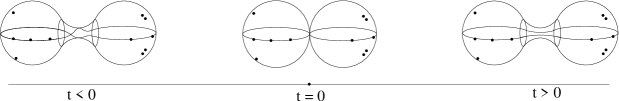
Figure 1: Two possible deformations of a real nodal point

.

3.3 Moduli space of $\sigma$-invariant curves

The moduli space $\overline{M}_{\mathbf{S}}(\mathbb{C})$ comes equipped with a natural real structure. The involution

$$c:(\Sigma;\mathbf{p})\mapsto(\overline{\Sigma};\mathbf{p})$$ (3)

gives the principal real structure of $\overline{M}_{\mathbf{S}}(\mathbb{C})$.

On the other hand, the permutation group $\mathbb{S}_{n}$ acts on $\overline{M}_{\mathbf{S}}(\mathbb{C})$ via relabeling: For each $\varrho\in\mathbb{S}_{n}$, there is an holomorphic map $\psi_{\varrho}$ defined by $(\Sigma;\mathbf{p})\mapsto(\Sigma;\varrho(\mathbf{p})):=(\Sigma;p_{\varrho(s_{1})},\cdots,p_{\varrho(s_{n})})$. For each involution $\sigma\in\mathbb{S}_{n}$, we have an additional real structure

$$c_{\sigma}:=c\circ\psi_{\sigma}:(\Sigma;\mathbf{p})\mapsto(\overline{\Sigma};\sigma(\mathbf{p}))$$ (4)

of $\overline{M}_{\mathbf{S}}(\mathbb{C})$. The real part $\overline{M}^{\sigma}_{\mathbf{S}}(\mathbb{R})$ of the real structure $c_{\sigma}:\overline{M}_{\mathbf{S}}(\mathbb{C})\to\overline{M}_{\mathbf{S}}(\mathbb{C})$ gives the moduli space of $\sigma$-invariant curves:

Theorem 5 (Ceyhan, c )

(a) For any $|\mathbf{S}|\geq 3$, $\overline{M}^{\sigma}_{\mathbf{S}}(\mathbb{R})$ is a smooth projective real manifold of dimension $|\mathbf{S}|-3$.

(b) Any $\sigma$-equivariant family $\pi_{B}:U_{B}(\mathbb{C})\to B(\mathbb{C})$ of $\mathbf{S}$-pointed stable curves is induced by a unique pair of real morphisms

$$\begin{CD}U_{B}(\mathbb{C})@>{\hat{\kappa}}>{}>\overline{U}_{\mathbf{S}}(\mathbb{C})\\ @V{\pi_{S}}V{}V@V{}V{\pi}V\\ B(\mathbb{C})@>{\kappa}>{}>\overline{M}_{\mathbf{S}}(\mathbb{C}).\end{CD}$$

(c) Let $\mathfrak{M}_{\sigma}(\mathbb{C})$ be the contravariant functor that sends each real variety $(B(\mathbb{C}),c_{B})$ to the set of $\sigma$-equivariant families of curves over $B(\mathbb{C})$. The moduli functor $\mathfrak{M}_{\sigma}(\mathbb{C})$ is represented by the real variety $(\overline{M}_{\mathbf{S}}(\mathbb{C}),c_{\sigma})$.

(d) Let $\mathfrak{M}_{\sigma}(\mathbb{R})$ be the contravariant functor that sends each real analytic manifold $R$ to the set of families of $\sigma$-invariant curves over $R$. The moduli functor $\mathfrak{M}_{\sigma}(\mathbb{R})$ is represented by the real part $\overline{M}^{\sigma}_{\mathbf{S}}(\mathbb{R})$ of $(\overline{M}_{\mathbf{S}}(\mathbb{C}),c_{\sigma})$.

Remark 3

The group of holomorphic automorphisms of $\overline{M}_{\mathbf{S}}(\mathbb{C})$ that respect its stratification is isomorphic to $\mathbb{S}_{n}$. Therefore, the real structures preserving the stratification of $\overline{M}_{\mathbf{S}}(\mathbb{C})$ are of the form (4) (see c ).

However, we don’t know whether there exist real structures other than (4), since the whole group of holomorphic automorphisms $Aut(\overline{M}_{\mathbf{S}}(\mathbb{C}))$ is not necessarily isomorphic to $\mathbb{S}_{n}$. For example, the automorphism group of $\overline{M}_{\mathbf{S}}(\mathbb{C})$ is $PSL_{2}(\mathbb{C})$ when $|\mathbf{S}|=4$.

It is believed that $Aut(\overline{M}_{\mathbf{S}}(\mathbb{C}))\cong\mathbb{S}_{n}$ for $|\mathbf{S}|\geq 5$. In fact, it is true for $|\mathbf{S}|=5$ and a proof can be found in dol . To the best of our knowledge, there is no systematic exposition of $Aut(\overline{M}_{\mathbf{S}}(\mathbb{C}))$ for $|\mathbf{S}|>5$.

3.4 A stratification of moduli space $\overline{M}^{\sigma}_{\mathbf{S}}(\mathbb{R})$

A stratification for $\overline{M}^{\sigma}_{\mathbf{S}}(\mathbb{R})$ can be obtained by using the stratification of $\overline{M}_{\mathbf{S}}(\mathbb{C})$ given in Theorem 1.

Lemma 1

Let $\gamma$ and $\overline{\gamma}$ be the dual trees of $(\Sigma;\mathbf{p})$ and $(\overline{\Sigma};\sigma(\mathbf{p}))$ respectively.

(a) If $\gamma$ and $\overline{\gamma}$ are not isomorphic, then the restriction of $c_{\sigma}$ on the union of complex strata $D_{\gamma}(\mathbb{C})\bigcup D_{\overline{\gamma}}(\mathbb{C})$ gives a real structure with empty real part.

(b) If $\gamma$ and $\overline{\gamma}$ are isomorphic, then the restriction of $c_{\sigma}$ on $D_{\gamma}(\mathbb{C})$ gives a real structure whose corresponding real part $D_{\gamma}(\mathbb{R})$ is the intersection of $\overline{M}^{\sigma}_{\mathbf{S}}(\mathbb{R})$ with $D_{\gamma}(\mathbb{C})$.

A tree $\gamma$ is called $\sigma$-invariant if it is isomorphic to $\bar{\gamma}$. We denote the set of $\sigma$-invariant $\mathbf{S}$-trees by $\mathcal{T}ree(\sigma)$.

Theorem 6 (Ceyhan, c )

$\overline{M}^{\sigma}_{\mathbf{S}}(\mathbb{R})$ is stratified by real analytic subsets

$$D_{\gamma}(\mathbb{R})=\prod_{v_{r}\in\mathbf{V}_{\gamma}^{\mathbb{R}}}M^{\hat{\sigma}}_{\mathbf{F}_{\gamma}(v_{r})}(\mathbb{R})\times\prod_{\{v,\overline{v}\}\subset\mathbf{V}_{\gamma}\setminus\mathbf{V}_{\gamma}^{\mathbb{R}}}M_{\mathbf{F}_{\gamma}(v)}(\mathbb{C})$$

where $\gamma\in\mathcal{T}ree(\sigma)$ and $\hat{\sigma}$ is the involution determined by the action of real structure $c_{\Sigma}$ on the special points labelled by $\mathbf{F}_{\gamma}(v_{r})$ for $v_{r}\in\mathbf{V}_{\gamma}^{\mathbb{R}}$.

Although the notion of $\sigma$-invariant trees leads us to a combinatorial stratification of $\overline{M}^{\sigma}_{\mathbf{S}}(\mathbb{R})$ as given in Theorem 6, it does not give a stratification in terms of connected strata. For a $\sigma$-invariant $\gamma$, the real part of the stratum $D_{\gamma}(\mathbb{R})$ has many connected components. A refinement of this stratification by using the spaces of $\mathbb{Z}_{2}$-equivariant point configurations in the projective line $\mathbb{P}^{1}(\mathbb{C})$.

$\mathbb{Z}_{2}$-equivariant configurations in $\mathbb{P}^{1}(\mathbb{C})$

Let $z:=[z:1]$ be an affine coordinate on $\mathbb{P}^{1}(\mathbb{C})$. Consider the upper half-plane $\mathbb{H}^{+}=\{z\in\mathbb{P}^{1}(\mathbb{C})\mid\Im{(z)}>0\}$ (resp. lower half plane $\mathbb{H}^{-}=\{z\in\mathbb{P}^{1}(\mathbb{C})\mid\Im{(z)}<0\}$) as a half of the $\mathbb{P}^{1}(\mathbb{C})$ with respect to $z\mapsto\bar{z}$, and the real part $\mathbb{P}^{1}(\mathbb{R})$ as its boundary. Denote by $\mathbb{H}$ the compactified disc $\mathbb{H}^{+}\cup\mathbb{P}^{1}(\mathbb{R})$.

The configuration space of $k=|\mathbf{Perm}(\sigma)|/2$ distinct pairs of conjugate points in $\mathbb{H}^{+}\bigsqcup\mathbb{H}^{-}$ and $l=|\mathbf{Fix}(\sigma)|$ distinct points in $\mathbb{P}^{1}(\mathbb{R})$ is

$${\widetilde{Conf}}_{(\mathbf{S},\sigma)} := \{(z_{s_{1}},\cdots,z_{s_{2k}};x_{r_{1}},\cdots,x_{r_{l}})\mid z_{s}\in\mathbb{H}^{+}\bigsqcup\mathbb{H}^{-}\ \mathrm{for}\ s\in\mathbf{F}\setminus\mathbf{F}^{\mathbb{R}},$$

$$z_{s}=z_{s^{\prime}}\Leftrightarrow s=s^{\prime},z_{s}=\bar{z}_{s^{\prime}}\Leftrightarrow s=\sigma(s^{\prime})\ \&$$

$$x_{r}\in\mathbb{P}^{1}(\mathbb{R})\ \mathrm{for}\ r\in\mathbf{Fix}(\sigma),\ x_{r}=x_{r^{\prime}}\Leftrightarrow r=r^{\prime}\}.$$

The number of connected components of ${\widetilde{Conf}}_{(\mathbf{S},\sigma)}$ is $2^{k}(l-1)!$ when $l\geq 2$, and $2^{k}$ when $l=1$. They are all diffeomorphic to each other; natural diffeomorphisms are given by $\sigma$-invariant relabelings.

The action of $SL_{2}(\mathbb{R})$ on $\mathbb{H}$ is given by

$$SL_{2}(\mathbb{R})\times\mathbb{H}\to\mathbb{H},\ \ (\Lambda,z)\mapsto\Lambda(z)=\frac{az+b}{cz+d},\ \ \Lambda=\left(\begin{array}[]{cc}a&b\\ c&d\\ \end{array}\right)\in SL_{2}(\mathbb{R}).$$ (7)

It induces an isomorphism $SL_{2}(\mathbb{R})/\pm I\to Aut(\mathbb{H})$. The automorphism group $Aut(\mathbb{H})$ acts on ${\widetilde{Conf}}_{(\mathbf{S},\sigma)}$ by

$$\Lambda:(z_{s_{1}},\cdots,z_{s_{2k}};x_{r_{1}},\cdots,x_{r_{l}})\mapsto(\Lambda(z_{s_{1}}),\cdots,\Lambda(z_{s_{2k}});\Lambda(x_{r_{1}}),\cdots,\Lambda(x_{r_{l}})).$$

This action preserves each of the connected components of ${\widetilde{Conf}}_{(\mathbf{S},\sigma)}$. It is free when $2k+l\geq 3$, and it commutes with diffeomorphisms given by $\sigma$-invariant relabelings. Therefore, the quotient space $\widetilde{C}_{(\mathbf{S},\sigma)}:={\widetilde{Conf}}_{(\mathbf{S},\sigma)}/Aut(\mathbb{H})$ is a manifold of dimension $2k+l-3$ whose connected components are pairwise diffeomorphic.

In addition to the automorphisms considered above, there is a diffeomorphism of ${\widetilde{Conf}}_{(\mathbf{S},\sigma)}$ which is given in affine coordinates as follows.

$$e:(z_{s_{1}},\cdots,z_{s_{2k}};x_{r_{1}},\cdots,x_{r_{l}})\mapsto(-z_{s_{1}},\cdots,-z_{s_{2k}};-x_{r_{1}},\cdots,-x_{r_{l}}).$$

Consider the quotient space $Conf_{(\mathbf{S},\sigma)}={\widetilde{Conf}}_{(\mathbf{S},\sigma)}/(e)$. The diffeomorphism $e$ commutes with each $\varrho$-invariant relabeling and normalizing action of $Aut(\mathbb{H})$. Therefore, the quotient space $C_{(\mathbf{S},\sigma)}:=Conf_{(\mathbf{S},\sigma)}/Aut(\mathbb{H})$ is a manifold of dimension $2k+l-3$, its connected components are diffeomorphic to the components of $\widetilde{C}_{(\mathbf{S},\sigma)}$, and, moreover, the quotient map $\widetilde{C}_{(\mathbf{S},\sigma)}\to C_{(\mathbf{S},\sigma)}$ is a trivial double covering.

Connected Components of $M^{\sigma}_{S}(\mathbb{R})$

Each connected component of $C_{(\mathbf{S},\sigma)}$ is associated to an unoriented combinatorial type of $\sigma$-invariant curves, and each unoriented combinatorial type is given by a one-vertex u-planar tree $\boldsymbol{\gamma}$. We denote the connected components of $C_{(\mathbf{S},\sigma)}$ by $C_{\boldsymbol{\gamma}}$.

Every $\mathbb{Z}_{2}$-equivariant point configuration defines a $\sigma$-invariant curve. Hence, we define

$$\Xi:\bigsqcup_{\boldsymbol{\gamma}:|\mathbf{V}_{\gamma}|=1}C_{\boldsymbol{\gamma}}\to M^{\sigma}_{\mathbf{S}}(\mathbb{R})$$ (8)

which maps $\mathbb{Z}_{2}$-equivariant point configurations to the corresponding isomorphisms classes of irreducible $\sigma$-invariant curves.

Lemma 2

(a) The map $\Xi$ is a diffeomorphism.

(b) Let $|\mathbf{Perm}(\sigma)|=2k$ and $\mathbf{Fix}(\sigma)=l$. The configuration space $C_{\boldsymbol{\gamma}}$ is diffeomorphic to

• $((\mathbb{H}^{+})^{k}\setminus\Delta)\times\mathbb{R}^{l-3}$ when $l>2$,

• $((\mathbb{H}^{+}\setminus\{\sqrt{-1}\})^{k-1}\setminus\Delta)\times\mathbb{R}^{l-1}$ when $l=1,2$,

where $\Delta$ is the union of all diagonals where $z_{s}=z_{s^{\prime}}$.

Refinement of the stratification

We associate a product of configuration spaces $C_{\widetilde{\boldsymbol{\gamma}}_{v}}$ and moduli spaces of pointed complex curves $\overline{M}_{\mathbf{F}_{\gamma}(v)}(\mathbb{C})$ to each o-planar tree $\widetilde{\boldsymbol{\gamma}}$:

$$C_{\widetilde{\boldsymbol{\gamma}}}=\prod_{v\in\mathbf{V}_{\gamma}^{\mathbb{R}}}C_{\boldsymbol{\gamma}_{v}}\times\prod_{v\in\mathbf{V}_{\gamma}^{+}}M_{\mathbf{F}_{\gamma}(v)}(\mathbb{C}).$$

For each u-planar $\boldsymbol{\gamma}$, we first choose an o-planar representative $\widetilde{\boldsymbol{\gamma}}$, and then we set $C_{\boldsymbol{\gamma}}:=C_{\widetilde{\boldsymbol{\gamma}}}$. Note that $C_{\boldsymbol{\gamma}}$ does not depend on the o-planar representative.

Theorem 7 (Ceyhan, c )

(a) $\overline{M}^{\sigma}_{\mathbf{S}}(\mathbb{R})$ is stratified by $C_{\boldsymbol{\gamma}}$.

(b) A stratum $C_{\boldsymbol{\gamma}}$ is contained in the boundary of $\overline{C}_{\boldsymbol{\tau}}$ if and only if $\boldsymbol{\tau}$ is obtained by contracting an invariant set of edges of $\boldsymbol{\gamma}$. The codimension of $C_{\boldsymbol{\gamma}}$ in $\overline{C}_{\boldsymbol{\tau}}$ is $|\mathbf{E}_{\gamma}|-|\mathbf{E}_{\tau}|$.

3.5 Graph homology of $\overline{M}^{\sigma}_{\mathbf{S}}(\mathbb{R})$

In this section, we summarize the results from c1 . We a give a combinatorial complex generated by the strata of $\overline{M}^{\sigma}_{\mathbf{S}}(\mathbb{R})$ whose homology is isomorphic to the homology of $\overline{M}^{\sigma}_{\mathbf{S}}(\mathbb{R})$.

A graph complex of $\overline{M}^{\sigma}_{\mathbf{S}}(\mathbb{R})$

Let $\sigma\in\mathbb{S}_{n}$ be an involution such that $\mathbf{Fix}(\sigma)\neq\emptyset$. We define a graded group

$$\mathcal{G}_{d} = \left(\bigoplus_{\boldsymbol{\gamma}:|\mathbf{E}_{\gamma}|=|\mathbf{S}|-d-3}H_{\dim(C_{\boldsymbol{\gamma}})}(\overline{C}_{\boldsymbol{\gamma}},Q_{\boldsymbol{\gamma}};\mathbb{Z})\right)/I_{d},$$ (9)

$$= \left(\bigoplus_{\boldsymbol{\gamma}:|\mathbf{E}_{\gamma}|=|\mathbf{S}|-d-3}\mathbb{Z}\ [\overline{C}_{\boldsymbol{\gamma}}]\right)/I_{d}$$ (10)

where $[\overline{C}_{\boldsymbol{\gamma}}]$ are the (relative) fundamental classes of the strata $\overline{C}_{\boldsymbol{\gamma}}$ of $\overline{M}^{\sigma}_{\mathbf{S}}(\mathbb{R})$. Here, $Q_{\boldsymbol{\gamma}}$ denotes the union of the substrata of $\overline{C}_{\boldsymbol{\gamma}}$ of codimension one and higher.

For $|\mathbf{Perm}(\sigma)|<4$, the subgroup $I_{d}$ (for degree d) is the trivial subgroup. In all other cases (i.e., for $|\mathbf{Perm}(\sigma)|\geq 4$), the subgroup $I_{d}$ is generated by the following elements.

The generators of the ideal of the graph complex.

The following paragraphs $\mathfrak{R}$-1 and $\mathfrak{R}$-2 describe the generators of the ideal of the graph complex.

$\mathfrak{R}$-1. Degeneration of a real vertex.

Consider an o-planar representative $\widetilde{\boldsymbol{\gamma}}$ of a u-planar tree $\boldsymbol{\gamma}$ such that $|\mathbf{E}_{\gamma}|=|\mathbf{S}|-d-5$, and consider one of its vertices $v\in\mathbf{V}_{\gamma}^{\mathbb{R}}$ with $|v|\geq 5$ and $|\mathbf{F}^{+}_{\gamma}(v)|\geq 2$. Let $f_{i},\bar{f}_{i}\in\mathbf{F}_{\gamma}\setminus\mathbf{F}_{\gamma}^{\mathbb{R}}$ be conjugate pairs of flags for $i=1,2$ such that $f_{1},f_{2}\in\mathbf{F}_{\gamma}^{+}(v)$ of $\widetilde{\boldsymbol{\gamma}}$, and let $f_{3}\in\mathbf{F}_{\gamma}^{\mathbb{R}}$. Put $\mathbf{F}=\mathbf{F}_{\gamma}(v)\setminus\{f_{1},\bar{f}_{1},f_{2},\bar{f}_{2},f_{3}\}$

We define two u-planar trees $\boldsymbol{\gamma}_{1}$ and $\boldsymbol{\gamma}_{2}$ as follows.

The o-planar representative $\widetilde{\boldsymbol{\gamma}}_{1}$ of $\boldsymbol{\gamma}_{1}$ is obtained by inserting a pair of conjugate edges $e=(f_{e},f^{e})$, $\bar{e}=(f_{\bar{e}},f^{\bar{e}})$ into $\widetilde{\boldsymbol{\gamma}}$ at $v$ in such a way that $\widetilde{\boldsymbol{\gamma}}_{1}$ gives $\widetilde{\boldsymbol{\gamma}}$ when we contract the edges $e,\bar{e}$. Let $\boldsymbol{\partial}_{\gamma_{1}}(e)=\{\tilde{v},v^{e}\}$, $\boldsymbol{\partial}_{\gamma_{1}}(\bar{e})=\{\tilde{v},v^{\bar{e}}\}$. Then, the distribution of flags of $\widetilde{\boldsymbol{\gamma}}_{1}$ is given by $\mathbf{F}_{\gamma_{1}}(\tilde{v})=\mathbf{F}_{1}\cup\{f_{3},f_{e},f_{\bar{e}}\}$, $\mathbf{F}_{\gamma_{1}}(v^{e})=\mathbf{F}_{2}\cup\{f_{1},f_{2},f^{e}\}$ and $\mathbf{F}_{\gamma_{1}}(v^{\bar{e}})=\overline{\mathbf{F}}_{2}\cup\{\bar{f}_{1},\bar{f}_{2},f^{\bar{e}}\}$ where $(\mathbf{F}_{1},\mathbf{F}_{2},\overline{\mathbf{F}}_{2})$ is an equivariant partition of $\mathbf{F}$.

The o-planar representative $\widetilde{\boldsymbol{\gamma}}_{2}$ of $\boldsymbol{\gamma}_{2}$ is obtained by inserting a pair of real edges $e_{1}=(f_{e_{1}},f^{e_{1}})$, $e_{2}=(f_{e_{2}},f^{e_{2}})$ into $\widetilde{\boldsymbol{\gamma}}$ at $v$ in such a way that $\widetilde{\boldsymbol{\gamma}}_{2}$ produces $\widetilde{\boldsymbol{\gamma}}$ when we contract the edges $e_{1},e_{2}$. Let $\boldsymbol{\partial}_{\gamma_{2}}(e_{1})=\{\tilde{v},v^{e_{1}}\}$, $\boldsymbol{\partial}_{\gamma_{2}}(e_{2})=\{\tilde{v},v^{e_{2}}\}$. The sets of flags of $\widetilde{\boldsymbol{\gamma}}_{2}$ are $\mathbf{F}_{\gamma_{2}}(\tilde{v})=\widetilde{\mathbf{F}}_{1}\cup\{f_{3},f_{e_{1}},f_{e_{2}}\}$, $\mathbf{F}_{\gamma_{2}}(v^{e_{1}})=\widetilde{\mathbf{F}}_{2}\cup\{f_{1},\bar{f}_{1},f^{e_{1}}\}$, $\mathbf{F}_{\gamma_{2}}(v^{e_{2}})=\widetilde{\mathbf{F}}_{3}\cup\{f_{2},\bar{f}_{2},f^{e_{2}}\}$ where $(\widetilde{\mathbf{F}}_{1},\widetilde{\mathbf{F}}_{2},\widetilde{\mathbf{F}}_{3})$ is an equivariant partition of $\mathbf{F}$.

The u-planar trees $\boldsymbol{\gamma}_{1},\boldsymbol{\gamma}_{2}$ are the equivalence classes represented by $\widetilde{\boldsymbol{\gamma}}_{1},\widetilde{\boldsymbol{\gamma}}_{2}$ given above.

Then, we define

$$\mathcal{R}(\boldsymbol{\gamma};v,f_{1},f_{2},f_{3}):=\sum_{\boldsymbol{\gamma}_{1}}[\overline{C}_{\boldsymbol{\gamma}_{1}}]-\sum_{\boldsymbol{\gamma}_{2}}[\overline{C}_{\boldsymbol{\gamma}_{2}}],$$ (11)

where the summation is taken over all possible $\boldsymbol{\gamma}_{i},i=1,2$ for a fixed set of flags $\{f_{1},\bar{f}_{1},f_{2},\bar{f}_{2},f_{3}\}$.

$\mathfrak{R}$-2. Degeneration of a conjugate pair of vertices.

Consider an o-planar representative $\widetilde{\boldsymbol{\gamma}}$ of a u-planar tree $\boldsymbol{\gamma}$ such that $|\mathbf{E}_{\gamma}|=|\mathbf{S}|-d-5$, and a pair of its conjugate vertices $v,\bar{v}\in\mathbf{V}_{\gamma}\setminus\mathbf{V}_{\gamma}^{\mathbb{R}}$ with $|v|=|\bar{v}|\geq 4$. Let $f_{i}\in\mathbf{F}_{\gamma}(v),i=1,\cdots,4$ and $\bar{f}_{i}\in\mathbf{F}_{\gamma}(\bar{v})$ be the flags conjugate to $f_{i},i=1,\cdots,4$. Put $\mathbf{F}=\mathbf{F}_{\gamma}(v)\setminus\{f_{1},\cdots,f_{4}\}$. Let $(\mathbf{F}_{1},\mathbf{F}_{2})$ be a two-partition of $\mathbf{F}$, and $\overline{\mathbf{F}}_{1},\overline{\mathbf{F}}_{2}$ be the sets of flags that are conjugate to the flags in $\mathbf{F}_{1},\mathbf{F}_{2}$ respectively.

We define two u-planar trees $\boldsymbol{\gamma}_{1}$ and $\boldsymbol{\gamma}_{2}$ as follows.

The o-planar representative $\widetilde{\boldsymbol{\gamma}}_{1}$ of $\boldsymbol{\gamma}_{1}$ is obtained by inserting a pair of conjugate edges $e=(f_{e},f^{e})$, $\bar{e}=(f_{\bar{e}},f^{\bar{e}})$ to $\widetilde{\boldsymbol{\gamma}}$ at $v,\bar{v}$ in such a way that $\widetilde{\boldsymbol{\gamma}}_{1}$ produces $\widetilde{\boldsymbol{\gamma}}$ when we contract the edges $e,\bar{e}$. Let $\boldsymbol{\partial}_{\gamma_{1}}(e)=\{v_{e},v^{e}\}$, $\boldsymbol{\partial}_{\gamma_{1}}(\bar{e})=\{v_{\bar{e}},v^{\bar{e}}\}$. The sets of flags of $\widetilde{\boldsymbol{\gamma}}_{1}$ are $\mathbf{F}_{\gamma_{1}}(v_{e})=\mathbf{F}_{1}\cup\{f_{1},f_{2},f_{e}\}$, $\mathbf{F}_{\gamma_{1}}(v^{e})=\mathbf{F}_{2}\cup\{f_{3},f_{4},f^{e}\}$ and $\mathbf{F}_{\gamma_{1}}(v_{\bar{e}})=\overline{\mathbf{F}}_{1}\cup\{\bar{f}_{1},\bar{f}_{2},f_{\bar{e}}\}$, $\mathbf{F}_{\gamma_{1}}(v^{\bar{e}})=\overline{\mathbf{F}}_{2}\cup\{\bar{f}_{3},\bar{f}_{4},f^{\bar{e}}\}$.

The o-planar representative $\widetilde{\boldsymbol{\gamma}}_{2}$ of $\boldsymbol{\gamma}_{2}$ is also obtained by inserting a pair of conjugate edges into $\widetilde{\boldsymbol{\gamma}}$ at the same vertices $v,\bar{v}$, but the flags are distributed differently on vertices. Let $\boldsymbol{\partial}_{\gamma_{2}}(e)=\{v_{e},v^{e}\}$, $\boldsymbol{\partial}_{\gamma_{2}}(\bar{e})=\{v_{\bar{e}},v^{\bar{e}}\}$. Then, the distribution of the flags of $\widetilde{\boldsymbol{\gamma}}_{2}$ is given by $\mathbf{F}_{\gamma_{2}}(v_{e})=\mathbf{F}_{1}\cup\{f_{1},f_{3},f_{e}\}$, $\mathbf{F}_{\gamma_{2}}(v^{e})=\mathbf{F}_{2}\cup\{f_{2},f_{4},f^{e}\}$, $\mathbf{F}_{\gamma_{2}}(v_{\bar{e}})=\overline{\mathbf{F}}_{1}\cup\{\bar{f}_{1},\bar{f}_{3},f_{\bar{e}}\}$, and $\mathbf{F}_{\gamma_{2}}(v^{\bar{e}})=\overline{\mathbf{F}}_{2}\cup\{\bar{f}_{2},\bar{f}_{4},f^{\bar{e}}\}$.

The u-planar trees $\boldsymbol{\gamma}_{1},\boldsymbol{\gamma}_{2}$ are the equivalence classes represented by $\widetilde{\boldsymbol{\gamma}}_{1},\widetilde{\boldsymbol{\gamma}}_{2}$ given above.

We define

$$\mathcal{R}(\boldsymbol{\gamma};v,f_{1},f_{2},f_{3},f_{4}):=\sum_{\boldsymbol{\gamma}_{1}}[\overline{C}_{\boldsymbol{\gamma}_{1}}]-\sum_{\boldsymbol{\gamma}_{2}}[\overline{C}_{\boldsymbol{\gamma}_{2}}],$$ (12)

where the summation is taken over all $\boldsymbol{\gamma}_{1},\boldsymbol{\gamma}_{2}$ for a fixed set of flags $\{f_{1},\cdots,f_{4}\}$.

The ideal $I_{d}$ is generated by $\mathcal{R}(\boldsymbol{\gamma};v,f_{1},f_{2},f_{3})$ and $\mathcal{R}(\boldsymbol{\gamma};v,f_{1},f_{2},f_{3},f_{4})$ for all $\boldsymbol{\gamma}$ and $v$ satisfying the required conditions above.

The boundary homomorphism of the graph complex

We define the graph complex $\mathcal{G}_{\bullet}$ of the moduli space $\overline{M}^{\sigma}_{\mathbf{S}}(\mathbb{R})$ by introducing a boundary map $\partial:\mathcal{G}_{d}\to\mathcal{G}_{d-1}$

$$\partial\ [\overline{C}_{\boldsymbol{\tau}}]\ =\ \sum_{\boldsymbol{\gamma}}\ \pm\ [\overline{C}_{\boldsymbol{\gamma}}],$$ (13)

where the summation is taken over all u-planar trees $\boldsymbol{\gamma}$ which give $\boldsymbol{\tau}$ after contracting one of their real edges.

Theorem 8 (Ceyhan, c1 )

The homology of the graph complex $\mathcal{G}_{\bullet}$ is isomorphic to the singular homology $H_{*}(\overline{M}^{\sigma}_{\mathbf{S}}(\mathbb{R});\mathbb{Z})$ for $\mathbf{Fix}(\sigma)\neq\emptyset$.

Remark 4

In c1 , the graph homology is defined and a similar theorem is proved for $\mathbf{Fix}(\sigma)=\emptyset$ case. The generators of the ideal are slightly different in this case.

Remark 5

If $|\mathbf{S}|>4$ and $|\mathbf{Fix}(\sigma)|\neq 0$, then the moduli space $\overline{M}^{\sigma}_{\mathbf{S}}(\mathbb{R})$ is not orientable. A combinatorial construction of the orientation double covering of $\overline{M}^{\sigma}_{\mathbf{S}}(\mathbb{R})$ is given in c . A stratification of the orientation cover is given in terms of certain equivalence classes of o-planar trees. By following the same ideas above, it is possible to construct a graph complex generated by fundamental classes of the strata that calculates the homology of the orientation double cover of $\overline{M}^{\sigma}_{\mathbf{S}}(\mathbb{R})$.

Remark 6

In their recent preprint ehkr , Etingof et al calculated the cohomology algebra $H^{*}(\overline{M}^{\sigma}_{\mathbf{S}}(\mathbb{R});\mathbb{Q})$ in terms of generators and relations for the $\sigma=id$ case. Until this work, little was known about the topology of $\overline{M}^{\sigma}_{\mathbf{S}}(\mathbb{R})$ (except DJS ; de ; gm ; ka ).

The graph homology, in a sense, treats the homology of the moduli space $\overline{M}^{\sigma}_{\mathbf{S}}(\mathbb{R})$ in the complementary directions to ehkr : The graph complex provides a recipe to calculate the homology of $\overline{M}^{\sigma}_{\mathbf{S}}(\mathbb{R})$ in $\mathbb{Z}$ coefficent for all possible involutions $\sigma$, and it reduces to cellular complex of the moduli space $\overline{M}^{\sigma}_{\mathbf{S}}(\mathbb{R})$ for $\sigma=id$ (see de ; ka ). Moreover, our presentation is based on stratification of $\overline{M}^{\sigma}_{\mathbf{S}}(\mathbb{R})$ which suits for investigating Gromov-Witten-Welschinger classes.

The graph homology provides a set of homological relations between the classes of $\overline{D}_{\boldsymbol{\gamma}}(\mathbb{R})$ that are essential for quantum cohomology of real varieties:

Corollary 1

If $\tau$ is a $\sigma$-invariant tree, then

$$\partial\ [\overline{D}_{\tau}(\mathbb{R})]=\sum_{{\text{all\ possible}}\atop{\text{u-planar\ str.\ of}\ \boldsymbol{\gamma}}}\sum_{\boldsymbol{\gamma}}\pm[\overline{C}_{\boldsymbol{\gamma}}]=\sum_{\gamma}[\overline{D}_{\gamma}(\mathbb{R})]$$ (14)

is homologous to zero.

Corollary 2

If $\boldsymbol{\gamma}$ be an o-planar tree satisfying the condition required in $\mathfrak{R}$-1, then the sum

$$\sum_{{\text{all\ possible}}\atop{\text{u-planar\ str.\ of}\ \boldsymbol{\gamma}}}\mathcal{R}(\boldsymbol{\gamma};v,f_{1},f_{2},f_{3})=\sum_{\gamma_{1}}[\overline{D}_{\gamma_{1}}(\mathbb{R})]-\sum_{\gamma_{2}}[\overline{D}_{\gamma_{2}}(\mathbb{R})]$$ (15)

is homologous to zero.

Part II: Quantum cohomology of real varieties

In this part, we recall the definition of Gromov-Witten classes and quantum cohomology. Then, we introduce Welschinger classes and quantum cohomology of real varieties. Our main goal is to revise Horava’s attempt of quantum cohomology of real varieties by investigating the properties of Gromov-Witten and Welschinger invariants.

4 Gromov-Witten classes

Let $X$ be a projective algebraic manifold, and let $\beta\in H_{2}(X;\mathbb{Z})$ such that $(L\cdot\beta)\geq 0$ for all Kähler $L$. Let $\overline{M}_{\mathbf{S}}(X,\beta)$ be the set of isomorphism classes of $\mathbf{S}$-pointed maps $(\Sigma;\mathbf{p};f)$ where $\Sigma$ is a projective nodal curve of genus zero, $p_{s_{1}},\cdots,p_{s_{n}}$ are distinct smooth labeled points of $\Sigma$, and $f:\Sigma\to X$ is a morphism satisfying $f_{*}([\Sigma])=\beta$.

For each labelled point $s\in\mathbf{S}$, the moduli space stable maps $\overline{M}_{\mathbf{S}}(X,\beta)$ inherits a canonical evaluation map

$$ev_{s}:\overline{M}_{\mathbf{S}}(X,\beta)\to X$$

defined for $(\Sigma;\mathbf{p};f)$ in $\overline{M}_{\mathbf{S}}(X,\beta)$ by:

$$ev_{s}:(\Sigma;\mathbf{p},f)\mapsto f(p_{s}).$$

Given classes $\mu_{s_{1}},\cdots,\mu_{s_{n}}\in H^{*}(X)$, a product is determined in the ring $H^{*}\overline{M}_{\mathbf{S}}(X,\beta)$ by:

$$ev^{*}_{s_{1}}(\mu_{s_{1}})\cup\cdots\cup ev^{*}_{s_{n}}(\mu_{s_{n}}).$$ (16)

If $\sum\text{codim}(\mu_{s})=\text{dim}(\overline{M}_{\mathbf{S}}(X,\beta))$, then the product (16) can evaluated on the fundamental class of $\overline{M}_{\mathbf{S}}(X,\beta)$. In such a case, the Gromov-Witten invariant is defined as the degree of the evaluation maps:

$$\int_{\overline{M}_{\mathbf{S}}(X,\beta)}ev^{*}_{s_{1}}(\mu_{s_{1}})\cup\cdots\cup ev^{*}_{s_{n}}(\mu_{s_{n}}).$$

This gives an appropriate counting of parametrized curves genus zero, lying in a given homology class $\beta$ and satisfying certain incidence conditions encoded by $\mu_{s}$’s.

The above definition of Gromov-Witten invariants leads to a more general Gromov-Witten invariants in $H^{*}\overline{M}_{\mathbf{S}}$: Given classes $\mu_{s_{1}},\cdots,\mu_{s_{n}}$, we have

$$I_{\mathbf{S},\beta}^{X}(\mu_{s_{1}}\otimes\cdots\otimes\mu_{s_{n}})=\nu_{*}(ev^{*}_{s_{1}}(\mu_{s_{1}})\cup\cdots\cup ev^{*}_{s_{n}}(\mu_{s_{n}}))$$

where $\nu:\overline{M}_{\mathbf{S}}(X,\beta)\to\overline{M}_{\mathbf{S}}$ is the projection that forgets the morphisms $f:\Sigma\to X$ and stabilizes resultant pointed curve (if necessary). The set of multilinear maps

$$\{I^{X}_{\mathbf{S},\beta}:\bigotimes_{\mathbf{S}}H^{*}X\to H^{*}\overline{M}_{\mathbf{S}}\}$$

is called the (tree-level) system of Gromov-Witten classes.

4.1 Cohomological field theory

A two-dimensional cohomological field theory (CohFT) with coefficient field $\mathbb{K}$ consists of the following data:

• A $\mathbb{K}$-linear superspace (of fields) $\mathcal{H}$, endowed with an even non-degenerate pairing $g$.

• A family of even linear maps (correlators)

  $$\{I_{\mathbf{S}}:\bigotimes_{\mathbf{S}}\mathcal{H}\to H^{*}\overline{M}_{\mathbf{S}}\}$$ (17)

  defined for all $|\mathbf{S}|\geq 3$.

These data must satisfy the following axioms:

A. $\mathbb{S}_{n}$-covariance: The maps $I_{\mathbf{S}}$ are compatible with the actions of $\mathbb{S}_{n}$ on $\bigotimes_{\mathbf{S}}\mathcal{H}$ and on $\overline{M}_{\mathbf{S}}$.

B. Splitting: Let $\{\mu_{a}\}$ denote a basis of $\mathcal{H}$, $\Delta:=\sum g^{ab}\mu_{a}\otimes\mu_{b}$ is the Casimir element of the pairing.

Let $\mathbf{S}_{a}=\{s_{a_{1}},\cdots,s_{a_{m}}\}$, $\mathbf{S}_{b}=\{s_{b_{1}},\cdots,s_{b_{n}}\}$ and $\mathbf{S}=\mathbf{S}_{1}\sqcup\mathbf{S}_{2}$. Let $\gamma$ be an $\mathbf{S}$-tree such that $\mathbf{V}_{\gamma}=\{v_{a},v_{b}\}$, and the set of flags $\mathbf{F}_{\gamma}(v_{a})=\mathbf{S}_{a}\cup\{s_{a}\}$, $\mathbf{F}_{\gamma}(v_{b})=\mathbf{S}_{b}\cup\{s_{b}\}$, and let

$$\varphi_{\gamma}:\overline{M}_{\mathbf{F}_{\gamma}(v_{a})}\times\overline{M}_{\mathbf{F}_{\gamma}(v_{b})}\to\overline{M}_{\mathbf{S}}$$

be the map which assigns to the pointed curves $(\Sigma_{a};p_{s_{a_{1}}},\cdots,p_{s_{a_{m}}},p_{s_{a}})$ and $(\Sigma_{b};p_{s_{b_{1}}},\cdots,p_{s_{b_{n}}},p_{s_{b}})$, their union $\Sigma_{a}\cup\Sigma_{b}$ identified at $p_{s_{a}}$ and $p_{s_{b}}$.

The Splitting Axiom reads:

$$\varphi_{\gamma}^{*}(I_{\mathbf{S}}(\mu_{s_{1}}\cdots\mu_{s_{n}}))$$

$$=\varepsilon(\gamma)\sum_{a,b}\ g^{ab}\ I_{\mathbf{F}_{\gamma}(v_{a})}(\bigotimes_{\mathbf{S}_{a}}\mu_{s_{*}}\otimes\mu_{s_{a}}))\otimes I_{\mathbf{F}_{\gamma}(v_{a})}(\bigotimes_{\mathbf{S}_{b}}\mu_{s_{*}}\otimes\mu_{s_{b}}))$$ (18)

where $\varepsilon(\gamma)$ is the sign of permutation $(\mathbf{S}_{1},\mathbf{S}_{2})$ on $\{\mu_{*}\}$ of odd dimension.

CohFT’s are abstract generalizations of tree-level systems of Gromov-Witten classes: any system of GW-classes for a manifold $X$ satisfying appropriate assumptions gives rise to the cohomological field theory where $\mathcal{H}=H^{*}(X;\mathbb{K})$.

4.2 Homology operad of $\overline{M}_{\mathbf{S}}$

There is another useful reformulation of CohFT. By dualizing (17), we obtain a family of maps

$$\{\mathbf{Y}_{\mathbf{S}}:H_{*}\overline{M}_{\mathbf{S}\cup\{s\}}\to Hom(\bigotimes_{\mathbf{S}}\mathcal{H},\mathcal{H})\}.$$ (19)

Therefore, any homology class in $\overline{M}_{\mathbf{S}\cup\{s\}}$ is interpreted as an $n$-ary operation on $\mathcal{H}$. The additive relations given in Section 2.2 and the splitting axiom (4.1) become identities between these operations i.e., $\mathcal{H}$ carries the structure of an algebra over the cyclic operad $H_{*}\overline{M}_{\mathbf{S}\cup\{s\}}$.

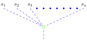
Figure 2: $n$-ary operation corresponding to the fundamental class of $\overline{M}_{\mathbf{S}\cup\{s\}}$

.

$Comm_{\infty}$-algebras

Each $n$-ary operation is a composition of $k$-ary operations corresponding to fundamental classes of $\overline{M}_{\mathbf{F}\cup\{s\}}$ for some $\mathbf{F}$ of order $k\leq n$. Reprehasing an algebra over $H_{*}\overline{M}_{\mathbf{S}\cup\{s\}}$-operad by using additive relations in $H_{*}\overline{M}_{\mathbf{S}\cup\{s\}}$ provides us a $Comm_{\infty}$-algebra.

The structure of $Comm_{\infty}$-algebra on $(\mathcal{H},g)$ is a sequence of even polylinear maps $\mathbf{Y}_{k}:\mathcal{H}^{\otimes k}\to A,k\geq 2$, satisfying the following conditions:

A^′. Higher commutativity: $\mathbf{Y}_{k}$ are $\mathbb{S}_{k}$-symmetric.

B^′. Higher associativity: For all $m\geq 0$, and $\mu_{\alpha},\mu_{\beta},\mu_{\delta},\mu_{i_{1}},\cdots,\mu_{i_{m}}\in A$, we have

$$\sum_{{\tau:\mathbf{S}_{1}\sqcup\mathbf{S}_{2}=\underline{\mathbf{n}}}\atop{\alpha,\beta,j_{*}\in\mathbf{S}_{1}\&\delta,k_{*}\in\mathbf{S}_{2}}}(-1)^{\varepsilon(\tau)}\mathbf{Y}_{|\mathbf{S}_{2}|}(\mathbf{Y}_{|\mathbf{S}_{1}|}(\mu_{\alpha},\mu_{\beta},\mu_{j_{1}},\cdots,\mu_{j_{r}}),\mu_{\delta},\mu_{k_{1}},\cdots,\mu_{k_{s}})$$

$$=\sum_{{\gamma:\mathbf{S}^{\prime}_{1}\sqcup\mathbf{S}^{\prime}_{2}=\underline{\mathbf{n}}}\atop{\beta,\delta,j_{*}\in\mathbf{S}^{\prime}_{2}\&\alpha,k_{*}\in\mathbf{S}^{\prime}_{1}}}(-1)^{\varepsilon(\gamma)}\mathbf{Y}_{|\mathbf{S}^{\prime}_{2}|}(\mathbf{Y}_{|\mathbf{S}^{\prime}_{1}|}(\mu_{\beta},\mu_{\delta},\mu_{j_{1}},\cdots,\mu_{j_{r}}),\mu_{\alpha},\mu_{k_{1}},\cdots,\mu_{k_{s}})$$

Here, the summations runs over all partitions of $\underline{\mathbf{n}}$ into two disjoint subsets $(\mathbf{S}_{1},\mathbf{S}_{2})$ and $(\mathbf{S}^{\prime}_{1},\mathbf{S}^{\prime}_{2})$ satisfying required conditions. Note that, these relations are consequences of the homology relations given in Theorem 2.

Since we identify the bases with $n$-corollas of the cyclic operad $H_{*}\overline{M}_{\mathbf{S}\cup\{s\}}$ (see, Figure 2), it is represented by as a linear span of all possible $\mathbf{S}^{\prime}$-trees modulo the higher associativity relations for $\mathbf{S}^{\prime}=\mathbf{S}\cup\{s\}$:

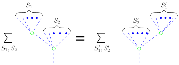
Figure 3: Higher associativity relations

.

We call $Comm_{\infty}$-algebra $(\mathcal{H},g,\mathbf{Y}_{*})$ cyclic if the tensors

$$\boldsymbol{\eta}_{k+1}:\mathcal{H}^{\otimes k+1}\to\mathbb{K},$$

$$\boldsymbol{\eta}_{k+1}(\mu_{1},\cdots,\mu_{k},\mu_{k+1}) :=g(\mathbf{Y}_{k}(\mu_{1},\cdots,\mu_{k}),\mu_{k+1})$$

are $\mathbb{S}_{k+1}$-symmetric .

4.3 Gromov-Witten potential and quantum product

Let $X$ be a manifold equipped with a system of tree level GW-classes. Put

$$\langle\mu_{s_{1}}\cdots\mu_{s_{n}}\rangle_{\beta}=\langle I_{\mathbf{S},\beta}^{X}\rangle(\mu_{s_{1}}\otimes\cdots\otimes\mu_{s_{n}}):=\int_{\overline{M}_{\mathbf{S}}}I_{\mathbf{S},\beta}^{X}(\mu_{s_{1}}\otimes\cdots\otimes\mu_{s_{n}}).$$

We define $\Phi$ as a formal sum depending on a variable point $\Gamma\in H^{*}(X)$:

$$\Phi(\Gamma):=\sum_{|\mathbf{S}|\geq 3}\sum_{\beta}\langle I_{\mathbf{S},\beta}^{X}\rangle(\Gamma^{\otimes|\mathbf{S}|})\frac{q^{\beta}}{|\mathbf{S}|!}.$$

The quantum multiplication is defined a product on tangent space of homology space $H^{*}(X)$ by

$$\partial_{a}*\partial_{b}=\sum_{c,d}\Phi_{abc}\ \partial_{d}$$

where $\Phi_{abc}$ denotes the third derivative $\partial_{a}\partial_{b}\partial_{c}(\Phi)$ of the potential function.

Theorem 9 (Kontsevich & Manin, km1 )

This definition makes the tangent sheaf of the homology space $H^{*}(X,\mathbb{C})$ a Frobenius manifold.

The main property, the associativity of quantum product is a consequence of splitting axiom of GW-classes and the defining relations of homology ring of $\overline{M}_{\mathbf{S}}$ (see, Theorem 2).

5 Gromov-Witten-Welschinger classes

In this section, we introduce the Welschinger classes by following the same principles and steps which lead to Gromov-Witten theory: Firstly, we introduce the real enumerative invariants in terms of homology of moduli space of suitable maps. Then, we transfer this definition to a new one in terms of the homology of $\overline{M}^{\sigma}_{\mathbf{S}}(\mathbb{R})$. We then further generalize our definition to open-closed CohFT’s and study these algebraic structures by using $H_{*}\overline{M}^{\sigma}_{\mathbf{S}}(\mathbb{R})$ i.e., introduce the quantum cohomology of real varieties.

5.1 Moduli space of stable real maps

Let $(X(\mathbb{C}),c_{X})$ be a projective real algebraic manifold. Let $\mathbf{d}:=(\beta,d)\in H_{2}(X(\mathbb{C}))\oplus H_{1}(X(\mathbb{R}))$.

We call a stable map $(\Sigma;\mathbf{p};f)\in\overline{M}_{\mathbf{S}}(X,\beta)$ $\sigma$-invariant if $\Sigma$ admits a real structure $c_{\Sigma}:\Sigma\to\Sigma$ such that $c_{\sigma}(p_{s})=p_{\sigma(s)}$, $c_{X}\circ f=f\circ c_{\Sigma}$ and $f_{*}([\Sigma(\mathbb{R})])=\pm d\in H_{1}(X(\mathbb{R}))$.

We denote the moduli space of $\sigma$-invariant stable maps by $\overline{R}^{\sigma}_{\mathbf{S}}(X,c_{X},\mathbf{d})$. The open stratum $R^{\sigma}_{\mathbf{S}}(X,c_{X},\mathbf{d})$ of $\overline{R}^{\sigma}_{\mathbf{S}}(X,c_{X},\mathbf{d})$ is a subspace of $\overline{R}^{\sigma}_{\mathbf{S}}(X,c_{X},\mathbf{d})$ where domain curve $\Sigma$ is irreducible. It is important to note that the moduli space $\overline{R}^{\sigma}_{\mathbf{S}}(X,c_{X},\mathbf{d})$ has boundaries. The $\sigma$-invariant maps $(\Sigma;\mathbf{p};f)$ lying in the boundaries have at least two components of domain curve $\Sigma$ which are not contracted to a point by morphism $f:\Sigma\to X$.

Obviously, $\overline{R}^{\sigma}_{\mathbf{S}}(X,c_{X},\mathbf{d})$ is a subspace of the real part of the real structure

$$c_{\sigma}:\overline{M}_{\mathbf{S}}(X,\beta)\to\overline{M}_{\mathbf{S}}(X,\beta);\ \ \ \ (\Sigma;\mathbf{p};f)\mapsto(\overline{\Sigma};\sigma(\mathbf{p});c_{X}\circ f).$$

Therefore, the restrictions of the evaluation maps provide us

$$\begin{array}[]{ll}ev_{s}:\overline{R}^{\sigma}_{\mathbf{S}}(X,c_{X},\mathbf{d})\to X(\mathbb{C}),&\ \text{for}\ s\in\mathbf{Perm}(\sigma),\\ ev_{s}:\overline{R}^{\sigma}_{\mathbf{S}}(X,c_{X},\mathbf{d})\to X(\mathbb{R}),&\ \text{for}\ s\in\mathbf{Fix}(\sigma).\end{array}$$

These moduli spaces have been extensively studied in the open Gromov-Witten invariants context. The compactification of these moduli spaces studied in (see fu ; liu ; s ). The orientibility of the open stratum $R^{\sigma}_{\mathbf{S}}(X,c_{X},\mathbf{d})$ has been noted first by Fukaya et al (for $\sigma=id$ case), Liu and (implicitly) by Welschinger in fu ; liu ; w1 ; w2 . Solomon treated this problem in most general setting (see s ).

5.2 Welschinger invariants as degrees of evalution maps

In a series of papers w1 -w4 , Welschinger defined a set of invariants counting, with appropriate weight $\pm 1$, real rational $J$-holomorphic curves intersecting a generic $\sigma$-invariant collection of marked points. Unlike the usual homological definition of Gromov-Witten invariants, Welschinger invariants are originally defined by assigning signs to individual curves based on certain geometric-topological criteria. A homological interpretation of Welschinger invariants has been given by J. Solomon very recently (see s ):

Let $H^{*}(X;\det(TX(\mathbb{R})))$ denote the cohomology of $X(\mathbb{R})$ with coefficients in the flat line bundle $\det(TX(\mathbb{R}))$. Let $\alpha_{s}\in\Omega^{*}(X(\mathbb{R}),TX(\mathbb{R}))$ be representatives of a set classes in $H^{*}(X;\det(TX(\mathbb{R})))$ for $s\in\mathbf{Fix}(\sigma)$. Furthermore, for $\{s,\bar{s}\}\subset\mathbf{Perm}(\sigma)$, $\mu_{s}\in\Omega^{*}X(\mathbb{C})$ represent a set of classes in $H^{*}(X(\mathbb{C}))$. Then, a product is determined in $\Omega^{*}R^{\sigma}_{\mathbf{S}}(X,c_{X},\mathbf{d})$ by

$$\bigwedge_{\{s,\overline{s}\}\subset\mathbf{Perm}(\sigma)}ev_{s}^{*}(\mu_{s})\ \wedge\ \bigwedge_{s\in\mathbf{Fix}(\sigma)}ev_{s}^{*}(\alpha_{s}).$$ (21)

If $\sum\text{codim}(\alpha_{*})+\sum\text{codim}(\mu_{*})=\dim(R^{\sigma}_{\mathbf{S}}(X,c_{X},\mathbf{d}))$, the form (21) extends along the critical locus of evaluation map except $\sigma$-invariant maps with reducible domain curve. In other words, it provides a relative cohomology class in $H^{*}(\overline{R}^{\sigma}_{\mathbf{S}}(X,c_{X},\mathbf{d}),\mathscr{D})$. Here, $\mathscr{D}$ is the subset of $\overline{R}^{\sigma}_{\mathbf{S}}(X,c_{X},\mathbf{d})$ whose elements $(\Sigma;\mathbf{p};f)$ have more than one components. This extension of the differential form (21) is a direct consequence of Welschinger’s theorems.

If $\mu_{*}$ and $\alpha_{*}$ are Poincare duals of point classes (respectively in $X(\mathbb{C})$ and $X(\mathbb{R})$), then one can define

$$N^{\sigma}_{\mathbf{S},\mathbf{d}}:=\int_{[\overline{R}^{\sigma}_{\mathbf{S}}(X,c_{X},\mathbf{d})]}\left\{\bigwedge_{\{s,\overline{s}\}\subset\mathbf{Perm}(\sigma)}ev_{s}^{*}(\mu_{s})\ \wedge\ \bigwedge_{s\in\mathbf{Fix}(\sigma)}ev_{s}^{*}(\alpha_{s})\right\}.$$ (22)

Proposition 1

(Solomon, s ) The sum

$$\sum_{d}N^{\sigma}_{\mathbf{S},\mathbf{d}}$$ (23)

which is taken over all possible homology classes $d\in H_{1}(X(\mathbb{R}))$ realized by $\sigma$-invariant maps, is equal to Welschinger invariants.

5.3 Welschinger classes

Let $\nu:\overline{R}^{\sigma}_{\mathbf{S}}(X,c_{X},\mathbf{d})\to\overline{M}^{\sigma}_{\mathbf{S}}(\mathbb{R})$ be the restriction of the contraction map $\nu:\overline{M}_{\mathbf{S}}(X,\beta)\to\overline{M}_{\mathbf{S}}$. Let $\mathfrak{D}$ be the subspace of $\overline{M}^{\sigma}_{\mathbf{S}}(\mathbb{R})$ whose elements $(\Sigma;\mathbf{p})$ has at least two irreducible components. Note that, the contraction morphism $\nu$ maps $\mathscr{D}\subset\overline{R}^{\sigma}_{\mathbf{S}}(X,c_{X},\mathbf{d})$ onto $\mathfrak{D}$.

By using the contraction morphism as in the definition of Gromov-Witten classes, Solomon’s definition of Welschinger invariants can be put into a more general setting:

$$W^{X}_{\mathbf{S},\mathbf{d}}(\bigotimes_{\{s,\bar{s}\}\subset\mathbf{Perm}(\sigma)}\mu_{s} \otimes \bigotimes_{s\in\mathbf{Fix}(\sigma)}\alpha_{s})$$

$$:= \nu_{*}(\bigwedge_{\{s,\overline{s}\}\subset\mathbf{Perm}(\sigma)}ev_{s}^{*}(\mu_{s})\ \wedge\ \bigwedge_{s\in\mathbf{Fix}(\sigma)}ev_{s}^{*}(\alpha_{s})).$$

The set of multilinear maps

$$W^{X}_{\mathbf{S},\mathbf{d}}:\bigotimes_{\mathbf{Perm}(\sigma)/\sigma}H^{*}(X(\mathbb{C}))\bigotimes_{\mathbf{Fix}(\mathbf{S})}H^{*}(X(\mathbb{R});\det(TX(\mathbb{R})))\to H^{*}(\overline{M}^{\sigma}_{\mathbf{S}}(\mathbb{R}),\mathfrak{D})$$

is called the system Welschinger classes.

5.4 Open-closed cohomological fields theory

An open-closed CohFT with coefficient field $\mathbb{K}$ consists of the following data:

• A pair of superspaces (of closed and open states) $\mathcal{H}_{c}$ and $\mathcal{H}_{o}$ endowed with even non-degenerate pairings $\eta_{c}$ and $\eta_{o}$ respectively.

• Two sets of linear maps (open & closed correlators)

  $$\{W_{\mathbf{S}}^{\sigma}: \bigotimes_{\mathbf{Perm}(\sigma)/\sigma}\mathcal{H}_{c}\otimes\bigotimes_{\mathbf{Fix}(\sigma)}\mathcal{H}_{o}\to H^{*}(\overline{M}^{\sigma}_{\mathbf{S}}(\mathbb{R}),\mathfrak{D})\}$$

  $$\{I_{\mathbf{S}}: \bigotimes_{\mathbf{S}}\mathcal{H}_{c}\to H^{*}(\overline{M}_{\mathbf{S}})\}$$

  defined for all $|\mathbf{S}|\geq 3$.

These data must satisfy the following axioms:

A^′. CohFT of closed states: The set of maps $\{I_{\mathbf{S}}:\bigotimes_{\mathbf{S}}\mathcal{H}_{c}\to H^{*}(\overline{M}_{\mathbf{S}})\}$ forms a CohFT.

B^′. Covariance: The maps $W_{\mathbf{S}}^{\sigma}$ are compatible with the actions of $\sigma$-invariant relabelling on $\bigotimes_{\mathbf{Perm}(\sigma)/\sigma}\mathcal{H}_{c}\otimes\bigotimes_{\mathbf{Fix}(\sigma)}\mathcal{H}_{o}$ and on $(\overline{M}^{\sigma}_{\mathbf{S}}(\mathbb{R}),\mathfrak{D})$.

C^′. Splitting 1: Let $\{\alpha_{a}\}$ denote a basis of $\mathcal{H}_{o}$, and let $\Delta_{o}$ be $\sum\eta_{o}^{ef}\alpha_{e}\otimes\alpha_{f}$.

Let $\gamma$ be a $\sigma$-invariant tree with $\mathbf{V}_{\gamma}=\mathbf{V}_{\gamma}^{\mathbb{R}}=\{v_{e},v_{f}\}$, and let $\mathbf{F}_{\gamma}(v_{e})=\mathbf{S}_{e}\cup\{s_{e}\}$, $\mathbf{F}_{\gamma}(v_{f})=\mathbf{S}_{f}\cup\{s_{f}\}$ and $\mathbf{S}=\mathbf{S}_{e}\cup\mathbf{S}_{f}$. We denote the restriction of $\sigma$ onto $\mathbf{S}_{e},\mathbf{S}_{f}$ by $\sigma_{e},\sigma_{f}$ respectively. Let

$$\phi_{\gamma}:\overline{D}_{\gamma}(\mathbb{R}):=\overline{M}^{\sigma_{e}}_{\mathbf{F}_{\gamma}(v_{e})}(\mathbb{R})\times\overline{M}^{\sigma_{f}}_{\mathbf{F}_{\gamma}(v_{f})}(\mathbb{R})\hookrightarrow\overline{M}^{\sigma}_{\mathbf{S}}(\mathbb{R})$$

be the embedding of the real divisor $\overline{D}_{\gamma}(\mathbb{R})$.

The Splitting Axiom reads:

$$\phi_{\gamma}^{*}(W_{\mathbf{S}}^{\sigma}(\bigotimes_{\mathbf{Perm}(\sigma)/\sigma}\mu_{*} \otimes \bigotimes_{\mathbf{Fix}(\sigma)}\alpha_{*}))$$

$$=\varepsilon(\gamma)\sum_{a,b} \eta_{o}^{ef} \ W^{\sigma_{e}}_{\mathbf{F}_{\gamma}(v_{e})}(\bigotimes_{\mathbf{Perm}(\sigma_{e})/\sigma_{e}}\mu_{*}\bigotimes_{\mathbf{Fix}(\sigma_{e})\setminus\{s_{e}\}}\alpha_{*}\otimes\alpha_{e})$$

$$\otimes W^{\sigma_{f}}_{\mathbf{F}_{\gamma}(v_{f})}(\bigotimes_{\mathbf{Perm}(\sigma_{f})/\sigma_{f}}\mu_{*}\bigotimes_{\mathbf{Fix}(\sigma_{f})\setminus\{s_{f}\}}\alpha_{*}\otimes\alpha_{f}).$$

D^′. Splitting 2: Let $\gamma$ be a $\sigma$-invariant tree with $\mathbf{V}_{\gamma}=\{v_{r},v,\bar{v}\}$ and $\mathbf{V}_{\gamma}^{\mathbb{R}}=\{v_{r}\}$, and let $\mathbf{F}_{\gamma}(v_{r})=\mathbf{S}_{r}\cup\{s_{e},\bar{s}_{e}\}$, $\mathbf{F}_{\gamma}(v)=\mathbf{S}_{f}\cup\{s_{f}\}$, $\mathbf{F}_{\gamma}(\bar{v})=\overline{\mathbf{S}}_{f}\cup\{\bar{s}_{f}\}$ and $\mathbf{S}=\mathbf{S}_{r}\cup\mathbf{S}_{f}\cup\overline{\mathbf{S}}_{f}$. We denote the restriction of $\sigma$ onto $\mathbf{S}_{r}$ by $\sigma_{r}$. Let

$$\phi_{\gamma}:\overline{D}_{\gamma}(\mathbb{R}):=\overline{M}^{\sigma_{r}}_{\mathbf{F}_{\gamma}(v_{r})}(\mathbb{R})\times\overline{M}_{\mathbf{F}_{\gamma}(v)}(\mathbb{C})\hookrightarrow\overline{M}^{\sigma}_{\mathbf{S}}(\mathbb{R})$$

be the embedding of the subspace $\overline{D}_{\gamma}(\mathbb{R})$.

Then, the Splitting Axiom reads:

$$\phi_{\gamma}^{*}(W_{\mathbf{S}}^{\sigma}(\bigotimes_{\mathbf{Perm}(\sigma)/\sigma}\mu_{*}\bigotimes_{\mathbf{Fix}(\sigma)}\alpha_{*}\otimes))=\varepsilon(\gamma)$$

$$\sum_{a,b}\ \eta_{c}^{ab}\ \ W^{\sigma_{r}}_{\mathbf{F}_{\gamma}(v_{r})}(\mu_{a}\bigotimes_{\mathbf{Perm}(\sigma_{r})/\sigma_{r}}\mu_{*}\bigotimes_{\mathbf{Fix}(\sigma_{r})}\alpha_{*}\otimes)\otimes I_{\mathbf{F}_{\gamma}(v)}(\mu_{b}\otimes\bigotimes_{\mathbf{S}_{f}}\mu_{*}).$$

Open-closed CohFT s are abstract generalizations of systems of Gromov- Witten-Welschinger classes: any system of GW-classes and Welschinger classes for a real variety $(X,c_{X})$ satisfying appropriate assumptions gives rise to the open-closed CohFT where $\mathcal{H}_{c}=H^{*}X(\mathbb{C})$ and $\mathcal{H}_{o}=H^{*}(X(\mathbb{R});\det(TX(\mathbb{R})))$.

5.5 Quantum cohomology of real varieties: A DG-operad

In this section, we first give a brief account of Horava’s attempt of defining quantum cohomology of real varieties. Then, we define quantum cohomology for real varieties as a DG-operad of the reduced graph complex of the moduli space $\overline{M}^{\sigma}_{\mathbf{S}\cup\{s\}}(\mathbb{R})$. The definition of this DG-operad is based of Gromov-Witten-Welschinger classes.

Quantum cohomology of real varieties: Horava’s approach

The quantum cohomology for real algebraic varieties has been introduced surprisingly early, in 1993, by P. Horava in ho . In his paper, Horava describes a $\mathbb{Z}_{2}$-equivariant topological sigma model on a real variety $(X,c_{X})$ whose set of physical observables in the is a direct sum of the cohomologies of $X(\mathbb{C})$ and $X(\mathbb{R})$:

$$\mathcal{H}_{c}\oplus\mathcal{H}_{o}:=H^{*}(X(\mathbb{C}))\oplus H^{*}(X(\mathbb{R})).$$ (25)

In the case of usual topological sigma models, the OPE-algebra is known to give a deformation of the cohomology ring of $X(\mathbb{C})$. One may thus wonder what the classical structure of $\mathcal{H}_{c}\oplus\mathcal{H}_{o}$ is, of which the quantum OPE-algebra can be expected to be a deformation. Notice first that there is a natural structure of an $\mathcal{H}_{c}$-module on $\mathcal{H}_{c}\oplus\mathcal{H}_{o}$. Indeed, to define a product of a cohomology class $\alpha$ of $X(\mathbb{R})$ with a cohomology class $\mu$ of $X(\mathbb{C})$, we will pull back the cohomology class $\mu$ by $i:X(\mathbb{R})\hookrightarrow X(\mathbb{C})$, and take the wedge product with $\alpha$. Equipped with this natural structure, the module (25) associated with the pair represented by a manifold $X(\mathbb{C})$ and a real structure of it, can be chosen as a (non-classical) equivariant cohomology ring in the sense of br . Horava required this equivariant cohomology theory to be recovered in the classical limit of the OPE-algebra of the equivariant topological sigma model.

By ignoring the degeneracy phenomena, the correlation functions of such a model count the number of equivariant holomorphic curves $f:\Sigma\to X(\mathbb{C})$ meeting a number of subvarieties of $X(\mathbb{C})$ and $X(\mathbb{R})$ in images of prescribed points of $\Sigma$. The analogue of the quantum cohomology ring is now a structure of $H^{*}(X(\mathbb{C}))$-module structure on $H^{*}(X(\mathbb{C}))\oplus H^{*}(X(\mathbb{R}))$ deforming cup product.

However, the degeneracy phenomena is the key ingredient which encodes the relations that deformed product structure should respect. In the following paragraph, we define quantum cohomology of real variety as a DG-operad in order to recover these relations.

Reduced graph complex

Let $\mathcal{G}_{\bullet}$ be the graph complex of $\overline{M}^{\sigma}_{\mathbf{S}}(\mathbb{R})$. The reduced graph complex $\mathcal{C}_{\bullet}$ of the moduli space $\overline{M}^{\sigma}_{\mathbf{S}}(\mathbb{R})$ is a subcomplex of $\mathcal{G}_{\bullet}$ given as follows:

• The graded group is

  $$\mathcal{C}_{d}=\left(\bigoplus_{{\gamma\ \text{are}\ \sigma-\text{invariant}}\atop{\&|\mathbf{E}_{\gamma}|=|\mathbf{S}|-d-3}}\mathbb{Z}\ [\overline{D}_{\gamma}(\mathbb{R})]\right)/\mathcal{I}_{d}$$ (26)

  where $[\overline{D}_{\gamma}(\mathbb{R})]$ are the (relative) fundamental class of the subspaces $\overline{D}_{\gamma}(\mathbb{R})$ of $\overline{M}^{\sigma}_{\mathbf{S}}(\mathbb{R})$. The ideal of relations $\mathcal{I}_{d}$ is generated by (15).

• The boundary homomorphism of the reduced graph complex is given by the restriction of the boundary homomorphism $\partial:\mathcal{G}_{d}\to\mathcal{G}_{d-1}$ of the graph complex $\mathcal{G}_{\bullet}$ (see 14).

Remark 7

There is an obvious monomorphism $H_{*}(\mathcal{C}_{\bullet})\to H_{*}(\mathcal{G}_{\bullet})$. A priori, the dualization of (• ‣ 5.4) requires rather whole homology group $H_{*}(\mathcal{G}_{\bullet})$ than a subgroup $H_{*}(\mathcal{C}_{\bullet})$. However, the covariance property of $W_{\mathbf{S}}^{\sigma}$ allows us restrict ourselves to subspaces $\overline{D}_{\gamma}(\mathbb{R})$ instead of the strata considered in Theorem 7.

DG-operad of reduced graph homology

Let $\mathcal{C}_{\bullet}$ be the reduced graph complex of $\overline{M}^{\sigma}_{\mathbf{S}\cup\{s\}}(\mathbb{R})$. By dualizing (• ‣ 5.4), we obtain a family of maps

$$\{\mathbf{Z}_{\mathbf{S}}^{\sigma}:\mathcal{C}_{\bullet}\to Hom(\bigotimes_{\mathbf{Perm}(\sigma)/\sigma}\mathcal{H}_{c}\bigotimes_{\mathbf{Fix}(\sigma)}\mathcal{H}_{o},\mathcal{H}_{o})\}$$ (27)

along with an algebra over $H_{*}\overline{M}_{\mathbf{S}\cup\{s\}}$-operad

$$\{\mathbf{Y}_{\mathbf{S}}:H_{*}\overline{M}_{\mathbf{S}\cup\{s\}}\to Hom(\bigotimes_{\mathbf{S}}\mathcal{H}_{c},\mathcal{H}_{c})\}.$$ (28)

Therefore, the homology class of subspace $\overline{D}_{\gamma}(\mathbb{R})$ in $\overline{M}^{\sigma}_{\mathbf{S}\cup\{s\}}(\mathbb{R})$ is interpreted as an $(k,l)$-ary operation on $\mathcal{H}_{o}\oplus\mathcal{H}_{c}$ where $k=|\mathbf{Perm}(\sigma)|/2$ and $l=|\mathbf{Fix}(\sigma)|$.

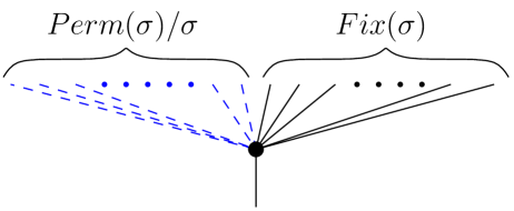
Figure 4: $(k,l)$-ary operation corresponding to the fundamental class of $\overline{M}^{\sigma}_{\mathbf{S}\cup\{s\}}(\mathbb{R})$

.

Remark 8

The $\sigma$-invariant trees which are used in Lemma 1 are different than the trees depict $(k,l)$-ary operation. These new trees are in fact are quotients of $\sigma$-invariant tree with respect to their symmetries arising from real structures of the corresponding $\sigma$-invariant curves.

In addition to the higher associativity $\mathbf{Y}_{\mathbf{S}}$, the additives relations in $\mathcal{C}_{\bullet}$ require additional conditions on $(k,l)$-ary operations. The families of maps $\mathbf{Z}_{\mathbf{S}}^{\sigma}$ and $\mathbf{Y}_{\mathbf{S}}$ satisfy the following conditions:

1. Higher associativiy relations: $(\mathcal{H}_{c},\eta_{c},\mathbf{Y}_{*})$ form a $Comm_{\infty}$-algebra structure.

2. $A_{\infty}$-type of structure: The additive relations arising from the image of the boundary homomorphism $\partial:\mathcal{C}_{*}\to\mathcal{C}_{*-1}$ (i.e., from the identity (14)) and the splitting axiom (C^′) become the following identities between $(k,l)$-ary operations:

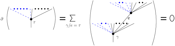
Figure 5: The image of boundary map provides $A_{\infty}$-type of relations

.

It is easy to see that $(A_{o},\eta_{o},\mathbf{Z}_{\mathbf{S}}^{\sigma})$ reduces to an $A_{\infty}$-algebra when $\sigma=id$.

2. Cardy type of relations: The additive relations arising from the ideal $\mathcal{I}_{d}$ of the graph complex $\mathcal{C}_{\bullet}$ (i.e., from the identity (15)) and the splitting axiom (D^′) become the following identities between $(k,l)$-ary operations:

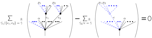
Figure 6: Cardy type of relations arising from the ideal $\mathcal{I}_{*}$

.

Here, $\hat{\gamma}_{1}.\hat{\gamma}_{2}$ are the quotients of $\gamma_{1},\gamma_{2}$ in (15) with respect to their $\mathbb{Z}_{2}$-symmetries induced by real structures of corresponding $\sigma$-invariant curves. In this picture, $\mu_{1},\mu_{2}$ correspond to the flags $f_{1},f_{2}$, and $\alpha$ corresponds to the real flag $f_{3}$.

Remark 9

The (partial) DG-operad defined above has close relatives which appeared in the literature.

The first one is Swiss-cheese operad which is introduced by Voronov in vo . In fact, Swiss-cheese operads are the chain operad of the spaces of $\mathbb{Z}_{2}$-equivariant configuration in $\mathbb{P}^{1}(\mathbb{C})$ (see, Section 3.4).

Kajiura and Stassheff recently introduced open-closed homotopy algebras which are amalgamations of $L_{\infty}$-algebras with $A_{\infty}$-algebras, see ks1 -ks3 . In their setting, the compactification of the configurations spaces are different than ours, therefore, the differential and the corresponding relations are different. In particular, there is no Cardy type of relation in their setting.

Very recently, Merkulov studied ‘operad of formal homogeneous space’ in mer . His approach is motivated by studies on relative obstruction theory, its applications (see r1 ; r2 ). It seems that a version of mirror symmetry which takes the real structures into account, has connection with this approach.

Part III: Yet again, mirror symmetry!

In his seminal paper kon , Kontsevich proposed that mirror symmetry is a (non-canonical) equivalence between the bounded derived category of coherent sheaves $D^{b}Coh(Y)$ on a complex variety $Y$ and the derived Fukaya category $DFuk(X)$ of its mirror, a symplectic manifold $(X,\omega)$. This first category consists of chain complexes of holomorphic bundles, with quasi-isomorphisms and their formal inverses. Roughly speaking, the derived Fukaya category should be constructed from Lagrangian submanifolds $L\subset X$ (carrying flat $U(1)$-connection $A$). Morphisms are given by Floer cohomology of Lagrangian submanifolds. One important feature is that, whereas the mirror of a Calabi-Yau variety is another Calabi-Yau variety, the mirrors of Fano varieties are Landau-Ginzburg models; i.e., affine varieties equipped with a map to called the superpotential.

Kontsevich also conjectured that the equivalence of derived categories should imply numerical predictions: For complex side (B-side), consider the diagonal subvariety $\Delta_{Y}\subset Y\times Y$, and define the Hochschild cohomology of $Y$ to be the endomorphism algebra of $\Delta_{Y}$ regarded as an object of $D^{b}Coh(X\times X)$ kon . Kontsevich interpreted the last definition of $HH^{*}(\mathcal{O}_{Y})$ ($\cong H^{*}(Y,\bigwedge^{*}TY)$) as computing the space of infinitesimal deformations of the bounded derived category of coherent sheaves on $Y$ in the class of $A_{\infty}$-categories. On the other hand, for symplectic side (A-side), the diagonal $\Delta_{X}\subset X\times X$ is a Lagrangian submanifold of $(X\times X,(\omega,-\omega))$. The Floer cohomology of the diagonal is canonically isomorphic to $H^{*}(X)$. Roughly, above picture suggests that deformation of $H^{*}(X)$ constructed using Gromov-Witten invariants should correspond to variations of Hodge structure in B-side.

‘Realizing’ mirror symmetry

Let $c_{X}:X\to X$ be an anti-symplectic involution of $(X,\omega)$. To recover more about real geometry from Kontsevich’s conjecture, we consider the structure sheaf $\mathcal{O}_{Y}$. Calculating its self-Hom’s

$$Ext^{i}(\mathcal{O}_{Y},\mathcal{O}_{Y})\cong H^{0,i}(Y)$$

shows that if $\mathcal{O}_{Y}$ is mirror to the Lagrangian submanifold $X(\mathbb{R})=\mathrm{Fix}(c_{X})$, then we must have

$$HF^{*}(X(\mathbb{R}),X(\mathbb{R}))\cong H^{0,*}(Y)$$

as graded vector spaces.

Kontsevich conjecture above and the description of quantum cohomology of real varieties that we have discussed in previous section, suggest us a correspondence between two ‘open-closed homotopy algebras’ (in an appropriate sense):

Symplectic side $X$  (A-side)	$\Longleftrightarrow$	Complex side $Y$  (B-side)
$(\mathcal{H}_{c},\mathcal{H}_{o})=$	$\Leftrightarrow$	$(\widehat{\mathcal{H}}_{c},\widehat{\mathcal{H}}_{o})=$
$(H^{*}(X),HF^{*}(X(\mathbb{R}),X(\mathbb{R})))$		$(H^{*,*}(Y),H^{0,*}(Y))$

If we restrict ourselves to three point operations, we apparently obtain $\mathcal{H}_{c}$ and $\widehat{\mathcal{H}}_{c}$-module structure in respective sides (which reminds Horava’s version of quantum cohomology of real varieties).

For A-side of the mirror correspondence, the DG-operad structure that we have discussed in previous section provides a promising candidate of extension this structure. However, the B-side of the story is more intriguing: Open-closed strings in B-model, their boundary conditions etc. are quite unclear to us. S. Merkulov pointed out possible connections with Ran’s work on relative obstructions, Lie atoms and their deformations r1 ; r2

References

- (1) G. Bredon, Equivariant Cohomology Theories. Lecture Notes in Mathematics 34, Springer Verlag, Berlin, 1967.
- (2) Ö. Ceyhan, On moduli of pointed real curves of genus zero. Proceedings 13th Gokova Geometry Topology Conference 2006, 1-38.
- (3) Ö. Ceyhan, On moduli of pointed real curves of genus zero. Ph.D. Thesis. IRMA Preprints. Ref: 06019.
- (4) Ö. Ceyhan, The graph homology of the moduli space of pointed real curves of genus zero. to appear in Selecta Mathematica.
- (5) Ö. Ceyhan, On Solomon’s reconstruction theorem for Gromov-Witten-Welshinger classes. in preperation.
- (6) Ö. Ceyhan, ‘Realizing’ mirror symmetry. in preperation.
- (7) M. Davis, T. Januszkiewicz, R. Scott, Fundamental groups of blow-ups. Adv. Math. 177 (2003), no. 1, 115–179.
- (8) A. Degtyarev, I. Itenberg, V. Kharlamov, Real enriques surfaces, Lecture Notes in Mathmetics 1746, Springer-Verlag, Berlin, 2000. xvi+259 pp.
- (9) S.L. Devadoss, Tessellations of moduli spaces and the mosaic operad. in ‘Homotopy invariant algebraic structures’ (Baltimore, MD, 1998), 91–114, Contemp. Math., 239, Amer. Math. Soc., Providence, RI, 1999.
- (10) I. Dolgachev, Topics in Classical Algebraic Geometry. Part I. lecture notes, available authors webpage http://www.math.lsa.umich.edu/ idolga/topics1.pdf
- (11) P. Etingof, A. Henriques, J. Kamnitzer, E. Rains, The cohomology ring of the real locus of the moduli space of stable curves of genus 0 with marked points. preprint math.AT/0507514.
- (12) K. Fukaya, Y.G. Oh, H. Ohta, K. Ono, Lagrangian intersection Floer theory: anomaly and obstruction. preprint 2000.
- (13) P. Griffiths, J. Harris, Principles of algebraic geometry. Pure and Applied Mathematics. Wiley-Interscience [John Wiley and Sons], New York, (1978). xii+813 pp.
- (14) A.B. Goncharov, Yu.I. Manin, Multiple -motives and moduli spaces . Compos. Math. 140 (2004), no. 1, 1–14.
- (15) J. Harris, I. Morrison, Moduli of curves. Graduate Texts in Mathematics vol 187, Springer-Verlag, NewYork, (1998), 366 pp.
- (16) A. Henriques, J. Kamnitzer, Crystals and coboundary categories. Duke Math. J. 132 (2006), no. 2, 191–216.
- (17) P. Horava, Equivariant topological sigma models. Nuclear Phys. B 418 (1994), no. 3, 571–602.
- (18) I. Itenberg, V. Kharlamov, E. Shustin, A Caporaso-Harris type formula for Welschinger invariants of real toric Del Pezzo surfaces. preprint math/0608549.
- (19) H. Kajiura, J. Stasheff, Jim Homotopy algebras inspired by classical open-closed string field theory. Comm. Math. Phys. 263 (2006), no. 3, 553–581.
- (20) H. Kajiura, J. Stasheff, Open-closed homotopy algebra in mathematical physics. J. Math. Phys. 47 (2006), no. 2, 023506, 28 pp.
- (21) H. Kajiura, J. Stasheff, Homotopy algebra of open-closed strings. hep-th/ 0606283.
- (22) M. Kapranov, The permutoassociahedron, MacLane’s coherence theorem and asymptotic zones for KZ equation. J. Pure Appl. Algebra 85 (1993), no. 2, 119–142.
- (23) S. Keel, Intersection theory of moduli space of stable N-pointed curves of genus zero, Trans. Amer. Math. Soc. 330 (1992), no. 2, 545–574.
- (24) M. Kontsevich, it Homological algebra of mirror symmetry. Proceedings of the International Congress of Mathematicians, Vol. 1, 2 (Zürich, 1994), 120–139, Birkhäuser, Basel, 1995.
- (25) M. Kontsevich, Yu.- I. Manin, Gromov-Witten classes, quantum cohomology, and enumerative geometry. Comm. Math. Phys. 164 (1994), no. 3, 525–562.
- (26) M. Kontsevich, Yu.-I. Manin (with appendix by R. Kaufmann), Quantum cohomology of a product. Invent. Math. 124 (1996), no. 1-3, 313–339.
- (27) F.F. Knudsen, The projectivity of the moduli space of stable curves. II. The stacks . Math. Scand. 52 (1983), no. 2, 161–199.
- (28) C.C.M. Liu, Moduli J-holomorphic curves with Lagrangian boundary conditions and open Gromov-Witten invariants for an -equivariant pair. preprint math.SG/0210257.
- (29) Yu.-I. Manin, Frobenius manifolds, quantum cohomology and moduli spaces. AMS Colloquium Publications vol 47, Providence, RI, (1999), 303 pp.
- (30) Yu.-I. Manin, Gauge Field Theories and Complex Geometry. Grundlehren der Mathematischen Wissenschaften 289, Springer-Verlag, Berlin, (1997), 346 pp.
- (31) S. A. Merkulov, Operad of formal homogeneous spaces and Bernoulli numbers. math/0708.0891.
- (32) G. Mikhalkin, Counting curves via lattice paths in polygons. C. R. Math. Acad. Sci. Paris 336 (2003), no. 8, 629–634.
- (33) G. Mikhalkin, Enumerative tropical algebraic geometry in . J. Amer. Math. Soc. 18 (2005), no. 2, 313–377.
- (34) R. Pandharipande, J. Solomon, J. Walcher, Disk enumeration on the quintic 3-fold. math.SG/0610901.
- (35) Z. Ran, Lie Atoms and their deformation theory. math/0412204.
- (36) Z. Ran, Bernoulli numbers and deformations of schemes and maps. math/ 0609223.
- (37) J. Solomon, Intersection theory on the moduli space of holomorphic curves with Lagrangian boundary conditions. math.SG/0606429.
- (38) J. Solomon, A differential equation for the open Gromov-Witten potential. a talk given at Real, tropical, and complex enumerative geometry workshop at CRM-Montreal.
- (39) A. Voronov, The Swiss-cheese operad. Homotopy invariant algebraic structures (Baltimore, MD, 1998), 365–373, Contemp. Math., 239, Amer. Math. Soc., Providence, RI, 1999.
- (40) J.Y. Welschinger, Invariants of real symplectic 4-manifolds and lower bounds in real enumerative geometry. Invent. Math. 162 (2005), no. 1, 195–234.
- (41) J.Y. Welschinger, Spinor states of real rational curves in real algebraic convex 3-manifolds and enumerative invariants. Duke Math. J. 127 (2005), no. 1, 89–121.
- (42) J.Y. Welschinger, Invariants of real symplectic four-manifolds out of reducible and cuspidal curves. Bull. Soc. Math. France 134 (2006), no. 2, 287–325.
- (43) J.Y. Welschinger, Towards relative invariants of real symplectic four-manifolds. Geom. Funct. Anal. 16 (2006), no. 5, 1157–1182.