Realization of the mean-field universality class in spin-crossover materials

Abstract

In spin-crossover materials, the volume of a molecule changes depending on whether it is in the high-spin (HS) or low-spin (LS) state. This change causes distortion of the lattice. Elastic interactions among these distortions play an important role for the cooperative properties of spin-transition phenomena. We find that the critical behavior caused by this elastic interaction belongs to the mean-field universality class, in which the critical exponents for the spontaneous magnetization and the susceptibility are $\beta=1/2$ and $\gamma=1$, respectively. Furthermore, the spin-spin correlation function is a constant at long distances, and it does not show an exponential decay in contrast to short-range models. The value of the correlation function at long distances shows different size-dependences: $O(1/N)$, $O(1/\sqrt{N})$, and constant for temperatures above, at, and below the critical temperature, respectively. The model does not exhibit clusters, even near the critical point. We also found that cluster growth is suppressed in the present model and that there is no critical opalescence in the coexistence region. During the relaxation process from a metastable state at the end of a hysteresis loop, nucleation phenomena are not observed, and spatially uniform configurations are maintained during the change of the fraction of HS and LS. These characteristics of the mean-field model are expected to be found not only in spin-crossover materials, but also generally in systems where elastic distortion mediates the interaction among local states.

I introduction

Spin-crossover (SC) materials consist of local units (molecules), each of which has two different spin states, i.e., the low-spin (LS) and high-spin (HS) states. The LS state is energetically favorable and dominates at low temperatures, while the HS state dominates at high temperatures because it is entropically favorable. The transition between the LS and HS states is also induced by changes of the pressure, magnetic field, light-irradiation, etc.Gutlich ; Decurtins ; Kahn ; Letard2 ; Hauser ; Real ; Shimamoto When interactions between molecules are weak, the HS fraction changes smoothly with temperature. However, when the interactions become strong, the system exhibits cooperative phenomena.Sorai1 The change in the HS fraction becomes sharper with increasing interaction. When the strength of the interaction exceeds a critical value, the change becomes discontinuous. In order to control electronic and magnetic properties of SC compounds, it is important to understand the bistable nature of such molecular solids.

As an important ingredient of the spin-crossover transition, we need two important characteristics of the system. One of them is the structure of the intra-molecule Hamiltonian. At each molecule, we set an energy difference between the states $D(>0)$ (see Fig. 1) and different degeneracies of the states: $g_{\rm HS}$ and $g_{\rm LS}$ for the HS state and the LS state, respectively. We express the spin state at the $i$-th site by $s_{i}$ which takes $-1$ for LS and $+1$ for HS. The intra-molecule (on-site) interaction is expressed by

$${H}_{0}={1\over 2}D\sum_{i}s_{i}.$$ (1)

If we take into account the effect of the degeneracy as a temperature dependent field, we can use an effective Hamiltonian with non-degenerate variables $\sigma_{i}=\pm 1$:

$${\cal H}_{\rm eff}=\frac{1}{2}\sum_{i}(D-k_{\rm B}T\ln g)\sigma_{i},$$ (2)

where $g=g_{\rm HS}/g_{\rm LS}$ denotes the degeneracy ratio between the HS and LS states.

The other important characteristic is the intermolecular interaction. For the cooperative property in the SC transition, until recently a short-range Ising-type interaction has been adopted in the so-called Wajnflasz-Pick (WP) model:Wajnflasz2

$${\cal H}=-J\sum_{\langle i,j\rangle}\sigma_{i}\sigma_{j}+\frac{1}{2}\sum_{i}(D-k_{\rm B}T\ln g)\sigma_{i}.$$ (3)

This type of model has successfully explained various aspects of the ordering processes.Bousseksou1 ; Kamel1 ; Nishino1 ; Nishino_dynamical ; Miya2 However, the origin of the interactions between the spin states has remained unclear. There are various plausible origins of the interaction.

As a possible interaction mechanism, the importance of elastic interactions has been pointed out.Zimmermann ; Kambara ; Adler ; Willenbacher ; Tchougreeff ; Spiering ; Nasser ; kbo The elastic constants may depend on the neighboring spin states. This dependence causes an effective interaction between the spin states. This effect of the elastic constants was investigated in a one-dimensional (1D) two-level modelNasser ; KBO2 and also in a 1D vibronic coupling model.kbo In these one-dimensional versions of the model, the elastic interactions can be traced out locally, leading to an exact mapping onto a 1D Ising ferromagnet, so that there is no phase transition at nonzero temperatures.kbo ; KBO2

In higher spatial dimensions, as depicted in the inset in Fig. 1, the volume change of a molecule causes a distortion of the lattice. Elastic interactions mediate the effect of this distortion over long distances. Therefore, in higher dimensions, the elastic interactions cause intrinsically different effects than in one dimension. We denote this long-range interaction by ${\cal H}_{\rm elastic}(\{\sigma_{i}\})$. We do not know the explicit form of this interaction. (But see discussion in Appendix B). However, we recently demonstrated that this type of elastic interaction can induce a phase transition in spin-crossover systems.Hawaii ; Nishino2007 ; Konishi2007 This elastic interaction model is a kind of compressible Ising model,Fisher1968 and similar models have been studied for binary alloys.Dunweg ; Laradji ; Zhu

Because the interaction originating from the elastic distortions is qualitatively different from that of the nearest-neighbor Ising model, we are interested in the critical properties of systems with this type of interaction. We have previously studied phase transitions and the temperature dependence of ordering of model SC materials with specified parameters $D$ and $g$. In those cases, most systems exhibit a first-order phase transition, and the critical properties of the models were not studied in detail. In the present study, we investigate properties near the critical point in the parameter space. In the case of the WP model, the critical properties are those of the short-range Ising ferromagnet. However, the critical properties of the present model, i.e., the critical exponents which characterize the critical universality, are expected to be different from those of the short-range Ising model.

The organization of the rest of this paper is as follows. In Sec. II we present the model and the computational method; in Sec. III we discuss the finite-size scaling analysis of the critical properties; in Sec. IV we discuss the spin configurations and correlations; and in Sec. V we present a summary and discussion. A discussion of the long-range Husimi-Temperley model is given in Appendix A, and a summary of finite-size scaling relations for mean-field phase transitions is given in Appendix B.

II Model and Method

In this paper, we study the critical phenomena of models with elastically mediated spin-spin interactions on the simple square lattice (2D), and also on the simple cubic lattice (3D) with periodic boundary conditions. Here we use Monte Carlo (MC) simulations according to the constant-pressure method.Konishi2007 In the Monte Carlo simulation, we choose a site $i$ randomly and update the spin state $\sigma_{i}=(\pm 1)$ and the position of the molecule$(x_{i},y_{i},z_{i})$ by the standard Metropolis method. We repeat this update $N$ times, where $N$ is the number of lattice sites. Then, we update the volume of the total system. We define this sequence of procedures to be one Monte Carlo step (MCS).

Instead of the Ising-like interactions of the WP model, Eq. (3), we adopt the following elastic interactions between molecules:Konishi2007

$$V = V_{\rm nn}+V_{\rm nnn}$$ (4)

$$V_{\rm nn} = \frac{k_{1}}{2}\sum_{\langle i,j\rangle}[r_{ij}-(R_{i}+R_{j})]^{2}$$ (5)

$$V_{\rm nnn} = \frac{k_{2}}{2}\sum_{\langle\langle i,j\rangle\rangle}[r_{ij}-\sqrt{2}(R_{i}+R_{j})]^{2},$$ (6)

where $r_{ij}$ is the distance between the $i$-th and $j$-th sites. $V_{\rm nn}$ expresses elastic interactions between nearest-neighbor pairs ($\langle i,j\rangle$). Here, $R_{i}$ and $R_{j}$ are the radii of the molecules. The radius of each molecule is $R_{\rm HS}$ and $R_{\rm LS}$ for the HS and LS states, respectively. In the present work, we set the ratio of the radii as $R_{\rm HS}/R_{\rm LS}=1.1$. $V_{\rm nnn}$ expresses the elastic interaction of next-nearest-neighbor pairs ($\langle\langle i,j\rangle\rangle$), which is necessary to maintain the lattice structure but not essential for the critical behavior. We set the ratio of the elastic constants $k_{1}/k_{2}=10$. We set $k_{1}=40$ through out the present work. In this study, in order to exclude other effects than those due to elastic interactions through distortion, we assume that the stiffness constants $k_{1}$ and $k_{2}$ do not depend on the spin state. If we were to allow spin dependence of $k_{1}$ and $k_{2}$, an effective short-range interaction would appear. In this sense, the present model treats only elastic interactions.

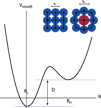
Figure 1: (Color online) Schematic picture of the energy structure of a molecule. The left (right) minimum corresponds to the LS (HS) state. In the inset, schematic pictures of a lattice of LS molecules (left), and the distortion caused by a HS molecule in a lattice of LS molecules (right) are illustrated.

The order parameter for the present model is the fraction of HS molecules, $f_{\rm HS}=N^{-1}\sum_{i}(2s_{i}-1)$. Hereafter, for convenience, we adopt the “magnetization,”

$$M=\sum_{i}^{N}s_{i}=\frac{N}{2}(f_{\rm HS}-1)$$ (7)

as the order parameter.

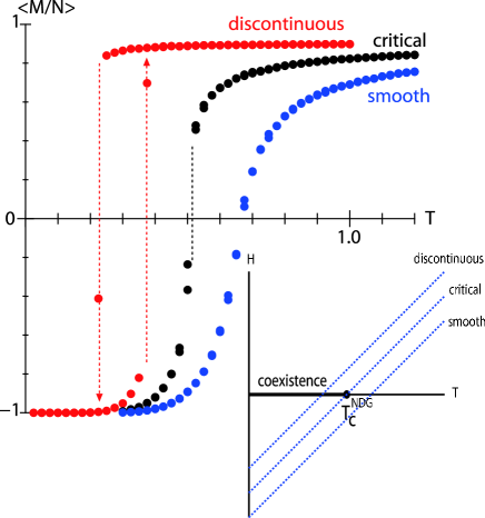
Figure 2: (Color online) The order parameter $\langle M\rangle/N$ vs temperature $T$ for $D=2$, 1.51, and 1. The temperature dependences are smooth, critical, and discontinuous (hysteresis), respectively. The inset shows a phase diagram of the model in the $(T,H)$ plane, where $T_{c}^{\rm NDG}$ is the critical temperature of the model ${\cal H}_{\rm elastic}$. The temperature changes in the model are given by the dotted lines in this phase diagram. When the dotted line crosses the coexistence line denoted by the bold line, the system undergoes a first-order phase transition.

In Fig. 2, we depict the temperature dependences of $\langle M\rangle$ for several values of $D$. Here, we find the typical $D$-dependences of $\langle M(T)\rangle$. That is, we find a smooth dependence for large values of $D$, and a first-order phase transition for small $D$. Between them, we have a second-order phase transition. This $D$-dependence is understood from the phase diagram of the non-degenerate model (i.e. $g=1$).Nishino1 In the present non-degenerate model a ferromagnetic phase transition takes place at $T_{c}^{\rm NDG}$, and we expect a phase diagram as shown in the inset. In this phase diagram, $H$ is the symmetry-breaking field.

The temperature dependences of the state of the present model with degeneracy $g>1$ (in this work we use $g=20$) are given by the dotted lines in the phase diagram,

$$H(T)={1\over 2}\left(D-k_{\rm B}T\ln g\right).$$ (8)

When $D$ is larger than $D_{\rm c}=k_{\rm B}T_{c}\ln g$, the temperature dependence of $\langle M\rangle$ is smooth, while it shows a first-order phase transition when $D<D_{\rm c}$. If we consider a specific material, the parameters $D$ and $g$ are given, and the temperature dependence of the state is given by one of these dotted lines. In most cases, the ordering is either smooth or discontinuous, and the critical properties have therefore not yet been seriously considered.

III Critical Properties

We study the critical properties of the elastically interacting model along the coexistence line given by $T=D/\ln g$, i.e. $H=0$.update For the WP model, the critical properties are those of the Ising model.

We next study the temperature (i.e., $T=D/k_{\rm B}T\ln g$) dependence of $\langle M^{2}\rangle$. The spontaneous magnetization $m_{s}$ and the susceptibility per spin $\chi$ are obtained from the relation

$${\langle M^{2}\rangle\over N^{2}}=m_{s}^{2}+k_{\rm B}T{\chi\over N},$$ (9)

where $N=L^{d}$ is the total number of spins, and

$$\chi={\langle M^{2}\rangle\over Nk_{\rm B}T},$$ (10)

which is the susceptibility per spin above the critical point. Here $\langle\cdots\rangle$ denotes the thermal average, i.e.,

$$\langle M^{2}\rangle={{\rm Tr}M^{2}e^{-\beta{\cal H}}\over{\rm Tr}e^{-\beta{\cal H}}}.$$ (11)

$$\begin{array}[]{c}\includegraphics[clip,width=156.49014pt]{M22D.eps}\\ ({\rm a})\\ \includegraphics[clip,width=156.49014pt]{M23D.eps}\\ ({\rm b})\end{array}$$

Figure 3: (Color online) Temperature dependences of ${\langle M^{2}\rangle/N^{2}}$ and the inverse susceptibility $\chi^{-1}=Nk_{\rm B}T/\langle M^{2}\rangle$. (a) A two-dimensional system (square lattice): ${\langle M^{2}\rangle/N^{2}}$ for the linear sizes $L=$ 10, 20, 30, and 50 are plotted by closed symbols of circle, square, diamond, and triangle, respectively; and $\chi^{-1}$ are plotted by the corresponding open symbols (multiplied by 20 for improved visibility). (b) A three-dimensional system (simple cubic lattice): ${\langle M^{2}\rangle/N^{2}}$ for $L=$ 8, 12, 16, and 20 are plotted by closed symbols of circle, square, diamond, and triangle, respectively; and $\chi^{-1}$ are plotted by the corresponding open symbols (multiplied by 5 for improved visibility). The dotted straight lines show the expected behaviors for a mean-field phase transition in an infinite system.

In Fig. 3, we depict the temperature dependences of ${\langle M^{2}\rangle/N^{2}}$, and $\chi^{-1}$. We find a clear linear dependence of ${\langle M^{2}\rangle/N^{2}}$ below $T\simeq 0.20$ for the 2D model, and $T\simeq 0.51$ for the 3D model. This linear dependence indicates that $m_{\rm s}^{2}\propto T_{c}-T$ and thus the critical exponent $\beta=1/2$.

In Fig. 3, we also find that $\chi^{-1}$ vanishes linearly at $T_{c}$, which indicates $\gamma=1$. This set of critical exponents agrees with those of the mean-field universality class. The size dependence of the inverse susceptibility in Fig. 3 is rather large, but we found similar size dependences of ${\langle M^{2}\rangle/N^{2}}$, and $\chi^{-1}$ in the long-range Husimi-Temperley model discussed in Appendix A. This indicates that the properties shown in Fig. 3 are inherent to models in the mean-field universality class.Fisher1968 ; Brezin-ZinnJustin ; Dunweg ; Laradji ; PRIV83 ; binder1985 ; Rikvold1993 ; Luijten-Bloete ; Zhu ; Jones

III.1 Binder Plot

We estimated the critical temperature by analysis of the Binder cumulant,binder

$$U_{4}=1-{\langle M^{4}\rangle\over 3\langle M^{2}\rangle^{2}}.$$ (12)

Plotted for different system sizes, this quantity has a crossing at the critical point. It has been extensively studied for the mean-field universality class.Brezin-ZinnJustin We depict the Binder plot in Fig. 4. The crossings are consistent with the values obtained from $\langle M^{2}\rangle/N^{2}$: $T_{c}\simeq 0.20$ for $d=2$ and $0.51$ for $d=3$. The value of $U_{4}$ at the crossing is universal and independent of the spatial dimension. It is in excellent agreement with the theoretical result,Brezin-ZinnJustin ; Luijten1995

$$U_{4}=1-{\Gamma^{4}(1/4)\over 24\pi^{2}}=0.27\cdots,$$ (13)

where $\Gamma$ is the Gamma function. In Appendix A, we show the Binder plot for the long-range Husimi-Temperley model, which gives the same fixed-point value.

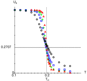
(a)

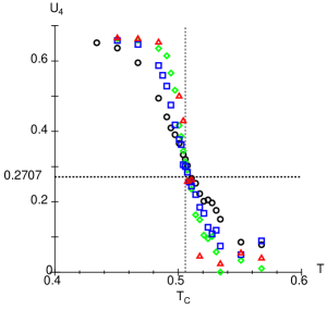
(b)

Figure 4: (Color online) Temperature dependence of the Binder cumulant. (a) A two-dimensional system (square lattice). Data for $L=$ 10, 20, 30, and 50 are plotted as circle, square, diamond, and triangle, respectively. (b) A three-dimensional system (simple cubic lattice). Data for $L=$ 8, 12, 16, and 20 are plotted as circle, square, diamond, and triangle, respectively.

III.2 Finite-size scaling

Finite-size scaling is one of the most useful methods to extract critical properties for infinite systems from numerical data for finite systems.PRIV84 ; PRIV90 However, special caution must be used when considering transitions in the mean-field universality class, which do not obey the hyperscaling relation $2\beta+\gamma=d\nu$ that relates the critical correlation-length exponent $\nu$ with the spatial dimensionality $d$ for transitions with nonclassical exponents.GOLD92 Essentially, lengths are not well defined in systems with mean-field phase transitions, and the linear system size $L$ is replaced by the number of sites $N$ as the fundamental finite-size scaling variable. A particularly clear example is the long-range Husimi-Temperley model discussed in Appendix A, in which every spin interacts with every other with a strength proportional to $1/N$. The finite-size scaling variable that replaces the standard $tL^{1/\nu}$ is $tN^{1/2}$.PRIV83 ; binder1985 This corresponds to an effective exponent $\nu^{*}=2/d$,PRIV83 ; Luijten-Bloete different from the value of $\nu=1/2$, obtained from the Gaussian approximation.GOLD92 An effective exponent for the correlation function on the large scales that are relevant for finite-size scaling is obtained from $\nu^{*}$ by the standard exponent relation $\eta^{*}=2-\gamma/\nu^{*}=(4-d)/2$. Thus one expects the scaling expression $\langle M^{2}\rangle=L^{d+2-\eta^{*}}\mathcal{M}^{2}(tL^{1/\nu^{*}})=L^{3d/2}\mathcal{M}^{2}(tL^{d/2})$, where $\mathcal{M}^{2}$ is a scaling function. A summary of the mechanisms that lead to these results is given in Appendix B.

In Fig. 5 we demonstrate that the Binder cumulants for different $L$ collapse onto a single scaling function when plotted vs $tL^{d/2}$,

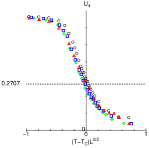
(a)

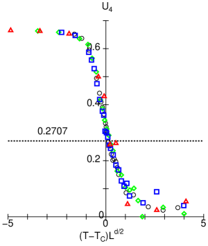
(b)

Figure 5: (Color online) Finite-size scaling plots of the Binder cumulant $U_{4}$ vs $(T-T_{c})L^{d/2}$. (a) The two-dimensional system. Data for $L=$ 10, 20, 30, and 50 are plotted as circle, square, diamond, and triangle, respectively. (b) The three-dimensional system. Data for $L=$ 8, 12, 16, and 20 are plotted as circle, square, diamond, and triangle, respectively.

and in Fig. 6 we plot the finite-size scaling functions for $\langle M^{2}\rangle$. In both cases we find good data collapse, both for $d=2$ and $d=3$. These finite-size scaling relationships are also seen in the long-range Husimi-Temperley model discussed in Appendix A.

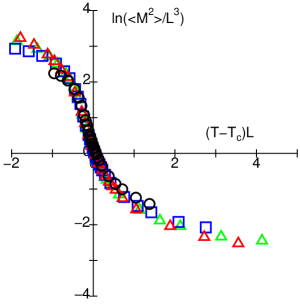
(a)

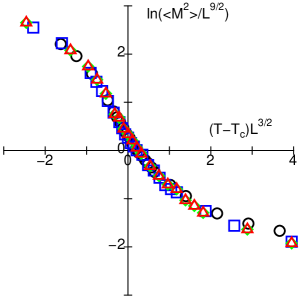
(b)

Figure 6: (Color online) Finite-size scaling plots of $\langle M^{2}\rangle$. (a) A two-dimensional system (square lattice). Data for $L=$ 10, 20, 30, and 50 are plotted as circle, square, diamond, and triangle, respectively. (b) A three-dimensional system (simple cubic lattice). Data for $L=$ 8, 12, 16, and 20 are plotted as circle, square, diamond, and triangle, respectively.

III.3 Phenomenological scaling analysis

In order to determine the critical temperature and the exponent $\eta^{*}=2-\gamma/\nu^{*}$, the so-called phenomenological Monte Carlo renormalization plot is often useful.PMCRG That is, we plot

$${\rm DLOG}={\ln\left(\langle M^{2}\rangle_{L}/\langle M^{2}\rangle_{L^{\prime}}\right)\over\ln(L/L^{\prime})}-d$$ (14)

as a function of $T$. The data for different sets of $L$ and $L^{\prime}$ are expected to cross at a point which gives $T_{c}$ and $\gamma/\nu^{*}=2-\eta^{*}$. In Fig. 7, we plot the temperature dependence of this quantity for two- and three-dimensional systems. We find a crossing in each figure at the position estimated by the values obtained in previous subsections: in the two-dimensional case,

$$T_{c}\simeq 0.20\quad{\rm and}\quad\eta^{*}\simeq 1,$$ (15)

and in the three-dimensional case,

$$T_{c}\simeq 0.51\quad{\rm and}\quad\eta^{*}\simeq 0.5.$$ (16)

We find a similar dependence in the Husimi-Temperley model given in Appendix A.

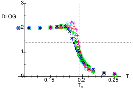
(a)

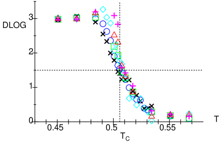
(b)

Figure 7: (Color online) Phenomenological Monte Carlo renormalization plots of $\langle M^{2}\rangle/N$, as defined in Eq. (14). (a) A two-dimensional system (square lattice). Data for $(L,L^{\prime})=$ (10,20), (10,30), (10,50), (20,30), (20,50), and (30,50) are plotted as cross, circle, square, diamond, triangle, and plus, respectively. (b) A three-dimensional system (simple cubic lattice). Data for $(L,L^{\prime})=$ (8,12), (8,16), (8,20), (12,16), (12,20), and (16,20) are plotted as cross, circle, square, diamond, triangle, and plus, respectively.

IV Spin Configuration

IV.1 Spin correlation function

(a)

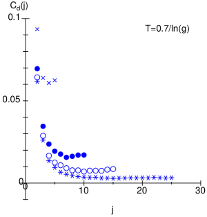
(b)

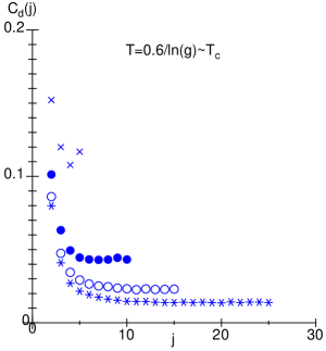
(c)

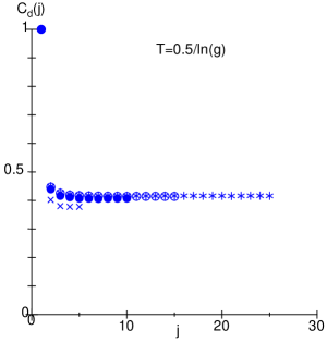
Figure 8: (Color online) The size and distance dependences of the spin correlation function in the two-dimensional model at several temperatures. (a) $T=0.7/\ln(g)$, which is in the paramagnetic phase. (b) $T=0.6/\ln(g)\sim T_{c}$. (c) $T=0.5/\ln(g)<T_{c}$ in the ordered phase. In these figures, the system sizes are $L=10~{}(\times)$, $20~{}(\bullet)$, $30~{}(\circ)$, and $50~{}(\ast)$.

Here, we concentrate on the characteristics of the spin correlation function. In Fig. 8, we depict the size and distance dependences of the correlation functions for various values of $T$: $T=0.7/\ln(g)$, which is in the paramagnetic phase, $T=0.6/\ln(g)\approx T_{c}$, and $T=0.5/\ln(g)<T_{c}$. We plot the correlation function along the diagonal direction, i.e., $C_{\rm d}(r)=\langle\sigma(x_{0},y_{0})\sigma(x_{0}+r,y_{0}+r)\rangle$.shotrange-order We find unusual spin correlation functions in the disordered phase. In short-range interaction models the correlation function decays exponentially. In contrast, we here find the correlation to be nonzero and almost constant at long distances in the disordered phase at $T=0.7/\ln(g)$. This observation indicates that the spins are strongly correlated, even at high temperatures. In the disordered phase, the susceptibility is an extensive quantity, and thus the total sum of the spin correlation function must be proportional to $N$:

$$N\chi T=\sum_{i}^{N}\sum_{j}^{N}\langle\sigma_{i}\sigma_{j}\rangle\propto N.$$ (17)

In order to satisfy this property, the constant value of the correlation function at long distances, $c_{0}$, must depend on the system size as

$$c_{0}\propto{1\over N}.$$ (18)

This is in stark contrast to the result for Ising models with short-range interactions, $c_{0}\sim e^{-L/2\xi}$ with a correlation length $\xi$ of order unity.

At the critical point ($T=0.6/\ln(g)\sim T_{c}$), the size dependence of $c_{0}$ is given by

$$c_{0}\propto{1\over\sqrt{N}}.$$ (19)

This constant component at the critical point was pointed out by Luijten and Blöte.Luijten-Bloete These observations are qualitatively different from those of the short-range Ising model. In the ordered state ($T=0.5/\ln(g)$), $c_{0}$ is independent of $N$, which corresponds to spontaneous order.

IV.2 Spin configuration in equilibrium

Next, let us discuss the characteristics of the spin configurations in the model. In Fig. 9, we depict three snapshots of spin configurations (a) at a high temperature, (b) near the critical point, and (c) at a low temperature.

$$\begin{array}[]{cc}\includegraphics[width=128.0374pt]{snap12tc.eps}&\includegraphics[width=128.0374pt]{snap10tc.eps}\\ ({\rm a})&({\rm b})\\ &\\ \includegraphics[clip,width=128.0374pt]{snap08tc.eps}&\includegraphics[width=128.0374pt]{ising-v0830-v2.eps}\\ ({\rm c})&({\rm d})\end{array}$$

Figure 9: (Color online) Snapshots of equilibrium configurations of the two-dimensional model at (a) $T=1.2T_{c}$, (b) $T=T_{c}$, and (c) $T=0.8T_{c}$. (d) A snapshot of the nearest-neighbor Ising ferromagnet near the critical point, $T=2.3J$.

We find that there are no large domain structures, even near the critical point. For comparison, we depict a configuration at the critical point of the two-dimensional nearest-neighbor Ising model (d). The difference is striking. We also found the structure factor to be almost wave-number independent (not shown). From these observations, we expect that usual critical behavior associated with two-phase coexistence will be suppressed in the present model.

IV.3 Spin configuration at the end of the hysteresis loop

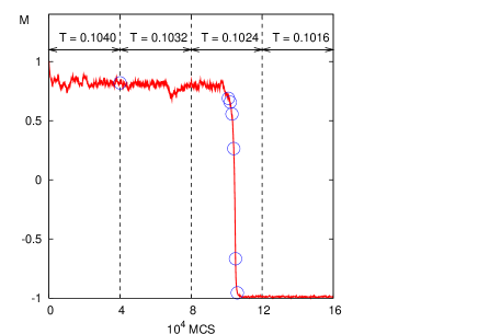
Figure 10: (Color online) Time dependence of the magnetization at the end of a hysteresis loop.

$$\begin{array}[]{cc}\includegraphics[width=128.0374pt]{hyst01-T026-D04-40000.eps}&\includegraphics[width=128.0374pt]{hyst03-T0256-D04-22000.eps}\\ ({\rm a})&({\rm b})\\ &\\ \includegraphics[width=128.0374pt]{hyst05-T0256-D04-23000.eps}&\includegraphics[width=128.0374pt]{hyst07-T0256-D04-24000.eps}\\ ({\rm c})&({\rm d})\\ &\\ \includegraphics[width=128.0374pt]{hyst09-T0256-D04-25000.eps}&\includegraphics[width=128.0374pt]{hyst11-T0256-D04-26000.eps}\\ ({\rm e})&({\rm f})\end{array}$$

Figure 11: (Color online) Time dependence of the spin configuration at the end of a hysteresis loop. (a) Configuration just before the end point, at $T=0.1040$. Here no change occurs after 40000 MCS. (b)At $T=0.1024$. At this temperature, a sudden change of the magnetization occurs at $22\,000$ MCS. (c) configuration at 23 000 MCS, (d) configuration at 24 000 MCS, (e) configuration at 25 000 MCS, (f) configuration at 26 000 MCS,

We also studied the change of the configuration at the end of a hysteresis loop, i.e., near the (pseudo)spinodal that marks the limit of the metastable HS phase. For this purpose, we decreased the temperature gradually from the HS phase in the two-dimensional model with $D=0.4$ ($<D_{c}\simeq 0.6$). The HS state remains as a metastable state beyond the coexistence curve. However at a certain point, it relaxes quickly to the LS state, marking the end of the hysteresis loop near the (pseudo)spinodal.UNGE84 In Fig. 10, we plot the time dependence of the magnetization as we decrease the temperature in steps by $\Delta T=0.008$ every 40 000 MCS. In the figure, the temperature is kept fixed at $T=0.1040$, 0.1032, 0.1024 and 0.1016. A rapid change of phase takes place at $T=0.1024$. In Fig. 11, we show configurations during this rapid change (denoted by circles in Fig. 10).

In contrast to short-range interaction models, in which the phase change occurs through nucleation and growth of compact critical droplets of the bulk equilibrium phase,RTMS the present system remains macroscopically uniform during the whole transformation process. This is consistent with the accepted picture of spinodal nucleation in systems with long-range interactions,UNGE84 ; MONE92 ; GORM94 ; KLEI02 ; GAGN05 ; KLEI07 where the critical droplet is known to be extended and highly ramified with a density close to that of the metastable phase. It is thus extremely difficult to distinguish from the metastable background. Growth of this critical droplet occurs by a filling-in of its “interior,” which is seen as the uniform change in the order parameter in Fig. 10.

IV.4 Spin configuration after quench into the low-temperature phase

In short-range models with non-conserved order parameter, the cluster size increases proportionally to the square-root of the elapsed time after a sudden quench from a disordered phase to a low-temperature phase.GUNT83 In contrast, the present model does not show such clustering configurations. In Fig. 12, we show a typical configuration after quenching.

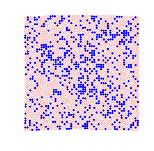
Figure 12: (Color online) A spin configuration at 200 MCS after a sudden change of $T$ ($T=10T_{c}$ to $T=0.8T_{c}$) along the symmetry line, $D=T\ln g$.

Here we again find no large cluster growth, which indicates that there is no critical opalescence in the present model.

These processes keeping uniformity can be understood in the following way. If a large domain exists, it causes a large distortion of the lattice, which is energetically unfavorable. Thus the system tends to be uniform on large length scales. This mechanism would be a characteristic of the present elastically induced mean-field phase transition. Beside the present SC system, there are various systems in which elastic interactions play an important role. For example, for the martensite transition in metals,martensite the elastic interaction is important, and we expect similar critical behavior there.

As mentioned previously, as far as a specific material is concerned, $D$ is given, and the temperature dependence of ordering is given by the dotted lines in Fig. 2. Thus, in most cases the phase transition is of first order. In such cases, the $D$ dependence of the ordering studied in this paper is difficult to observe. However, the fact that the system is always uniform and no clustering occurs should be observable, even in a specific material. Moreover, by making use of the pressure dependence,Konishi2007 we may also observe the critical properties and confirm the mean-field universality class.

V Summary and Discussion

We studied the critical properties of the elastically induced spin-crossover phase transition, finding it to belong to the mean-field universality class. The temperature dependences of the long-range order and the susceptibility were obtained in two- and three-dimensional models, and the corresponding critical exponents $\beta$ and $\gamma$ were found to be $1/2$ and $1$, respectively, in agreement with the mean-field universality class. The size- and temperature-dependence of $\langle M^{2}\rangle$ converged onto a scaling function. In the analysis of the finite-size scaling, we need critical exponents for the spin correlations, i.e., $\eta$ and $\nu$. We found that the effective values, $\eta^{*}=(4-d)/2$ and $\nu^{*}=2/d$, are good for the scaling plots, as has been pointed out in various studies of the mean-field universality class. We also found that the critical properties of our model agree well with the long-range interaction model (Husimi-Temperley model), in which the spin correlation function is constant at large distances.

We also studied characteristics of the spin configurations of the present model with effective long-range interactions. We found that the system does not show configurations with large clusters, even following sudden temperature quenches, or at the edge of the hysteresis loop near the (pseudo)spinodal. Thus critical opalescence and conventional nucleation phenomena do not appear in the present model. In materials, it is difficult to change $D$ or $g$, but the pressure dependence of these parametersKonishi2007 will enable them to be controlled, and we hope that the characteristic behaviors uncovered in this study will be found in real experiments in the future.

Appendix A: Finite size properties of the Husimi-Temperley model

We study the finite-size dependence of the magnetization of the Husimi-Temperley model as a reference of the mean-field type behavior. The Hamiltonian is given by

$${\cal H}=-{J\over N}\sum_{ij}\sigma_{i}\sigma_{j}=-{J\over N}\left(\sum_{i=1}^{N}\sigma_{i}\right)^{2}.$$ (20)

Following the standard method, we obtain the partition function:

$$Z={\rm Tr}e^{-\beta{\cal H}}=e^{{\beta J\over N}\left(\sum_{i=1}^{N}\sigma_{i}\right)^{2}}$$

$$={\rm Tr}\int_{-\infty}^{\infty}{dx\over\sqrt{2\pi}}e^{-{1\over 2}x^{2}+x\sqrt{2\beta J/N}\sum_{i=1}^{N}\sigma_{i}}$$

$$=\int_{-\infty}^{\infty}{dx\over\sqrt{2\pi}}e^{-{1\over 2}x^{2}+N\ln\left[2\cosh\left(x\sqrt{2\beta J/N}\right)\right]}$$

$$=\int_{-\infty}^{\infty}{\sqrt{N}dz\over\sqrt{2\pi}}e^{-{N\over 2}z^{2}+N\ln\left[2\cosh\left(z\sqrt{2\beta J}\right)\right]}$$ (21)

If we estimate this integral by the saddle-point method, we obtain the mean-field free energy

$$-{\beta F_{\rm MF}\over N}=-{1\over 2}z^{2}+\ln\left[2\cosh\left(z\sqrt{2\beta J}\right)\right].$$ (22)

Here, we obtain the physical quantities of the model for finite values of $N$. The average of the square of the magnetization is given by

$$\langle M^{2}\rangle={{\rm Tr}M^{2}e^{-\beta{\cal H}}\over{\rm Tr}e^{-\beta{\cal H}}}=N{\partial\over\partial\beta J}\ln Z$$

$$={\int_{-\infty}^{\infty}{\sqrt{N}dz\over\sqrt{2\pi}}N^{2}{z\over\sqrt{2\beta J}}\tanh\left(z\sqrt{2\beta J}\right)e^{-{N\over 2}z^{2}+N\ln\left[2\cosh\left(z\sqrt{2\beta J}\right)\right]}\over\int_{-\infty}^{\infty}{\sqrt{N}dz\over\sqrt{2\pi}}e^{-{N\over 2}z^{2}+N\ln\left[2\cosh\left(z\sqrt{2\beta J}\right)\right]}},$$ (23)

where

$$M=\sum_{i=1}^{N}\sigma_{i}.$$ (24)

The temperature dependence of $\langle M^{2}\rangle/N^{2}$ corresponds to the square of the spontaneous magnetization $m_{\rm s}$,

$$\lim_{N\rightarrow\infty}{\langle M^{2}\rangle\over N^{2}}=m_{\rm s}^{2},$$ (25)

and $k_{\rm B}TN/\langle M^{2}\rangle$ corresponds to the inverse susceptibility $\chi^{-1}$ above the critical temperature. We plot the data in Fig. 13. In the present model, the critical temperature is $2J/k_{\rm B}$. Hereafter we put $J=1$ and $k_{\rm B}=1$.

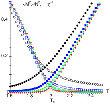
Figure 13: (Color online) Temperature dependence of $\langle M^{2}\rangle/N^{2}$ and the inverse susceptibility $\chi^{-1}=TN/\langle M^{2}\rangle$ for the Husimi-Temperley model. The circle, square, diamond, triangle and inverse-triangle denote $N=100$, 400, 900, 1600, and 2500, respectively. The open and closed symbols denote $\langle M^{2}\rangle/N$ and $\chi^{-1}$, respectively.

The Binder plot of this model is depicted in Fig. 14. We find that the data for large $N$ show a good crossing at $T_{c}$.

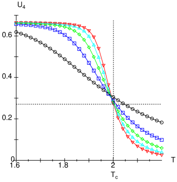
Figure 14: (Color online) The Binder plot for the Husimi-Temperley model. The circle, square, diamond, triangle and inverse-triangle denote $N=100,400,900,1600$ and 2500, respectively.

The following size dependences are easily obtained:

$$\langle M^{2}\rangle\propto\left\{\begin{array}[]{cc}N^{2}&{T<T_{c}},\\ N^{3/2}&\quad{T=T_{c}},\\ N&{T>T_{c}}.\end{array}\right.$$ (26)

The size- and temperature dependence of $\langle M^{2}\rangle$ is found to converge in the standard finite size scaling plot as depicted in Fig. 15. The values of the correlation functions at large separations in Eq. (18) and Eq. (19) correspond to the above size dependences.

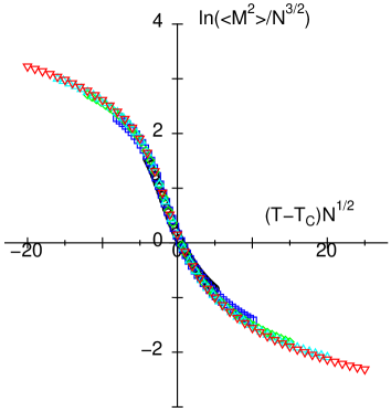
Figure 15: (Color online) The scaling plot of $\langle M^{2}\rangle$ for the Husimi-Temperley model. The circle, square, diamond, triangle and inverse-triangle denote $N=100$, 400, 900, 1600, and 2500, respectively.

These figures qualitatively agree well with those for the model of the elastic interaction mediated spin-crossover materials.

In Fig. 16 we plot the phenomenological scaling plot of the present data

$${\rm DLOG}={\ln{\langle M^{2}\rangle_{L}/\langle M^{2}\rangle_{L}^{\prime}}\over\ln{L/L^{\prime}}},$$ (27)

for various sets of $(L,L^{\prime})$. Here, we define $L=N^{1/2}$. In general, if we use a definition $L=N^{1/d}$, DLOG becomes DLOG$\times(d/2)$.

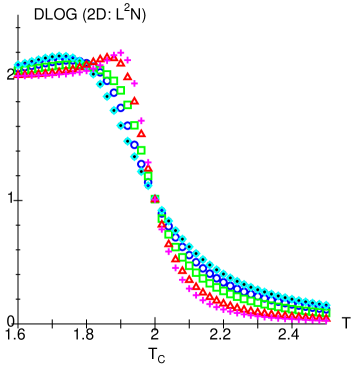
Figure 16: The phenomenological renormalization plot for the Husimi-Temperley model. Data for $(L,L^{\prime})=$ (10,20), (10,30), (10,50), (20,30), (20,50), and (30,50) are plotted by cross, circle, square, diamond, triangle, and plus, respectively.

Appendix B: Finite-size scaling of the mean-field model

In this Appendix we summarize the finite-size scaling properties expected in a spatially extended system with mean-field behavior, which agree with those observed numerically in this paper.

A $d$-dimensional $\phi^{4}$ lattice field theory with interaction range $\mathcal{R}$ can be defined by the Ginzburg-Landau Hamiltonian in reciprocal space,

$$\frac{\tilde{{\mathcal{H}}}(\phi_{\bf k})}{k_{\rm B}T} = \frac{1}{2}\sum_{\bf k}\left[(\mathcal{R}k)^{\sigma}-t\right]\phi_{\bf k}\phi_{-{\bf k}}$$ (28)

$$+\frac{u}{4N}\sum_{{\bf k}_{1},{\bf k}_{2},{\bf k}_{3}}\phi_{{\bf k}_{1}}\phi_{{\bf k}_{2}}\phi_{{\bf k}_{3}}\phi_{-({\bf k}_{1}+{\bf k}_{2}+{\bf k}_{3})}$$

$$-h\sqrt{\frac{N}{2}}\phi_{{\bf k}={\bf 0}}\;,$$

where $N=L^{d}$ is the number of lattice points, $t=(T-T_{c})/T_{c}$, and $h$ is an applied magnetic field. For $\sigma=2$ and constant $\mathcal{R}$, this model has local interactions and upper critical dimension $d_{u}=4$. For $d>4$ it has classical mean-field critical exponents, for $d=4$ it has mean-field exponents with logarithmic corrections, and for $d<4$ it has nontrivial critical exponents corresponding to the $d$-dimensional Ising universality class.Luijten-Bloete

For $d$ below four there are several ways the model can be modified to show mean-field critical behavior. One is to keep $\sigma=2$ fixed and let $\mathcal{R}\rightarrow\infty$ while using a scaling ansatz equivalent to a Ginzburg criterion,Rikvold1993 as is often done in studies of crossover scaling.LUIJ98 In this limit of infinitely weak, infinitely long-ranged interactions, the model reduces to the Husimi-Temperley model discussed in Appendix A. However, the method most relevant to elastic systemsTEOD82 ; PEYL99 ; PEYL03 ; UEMU01 is probably to increase the interaction range by modifying $\sigma$.Luijten-Bloete For $0\leq\sigma<d/2$, this lowers the upper critical dimension to

$$d_{u}(\sigma)=2\sigma$$ (29)

and leads to classical mean-field critical behavior for $d>d_{u}(\sigma)$. (As for $\sigma=2$, classical exponents with logarithmic corrections are found for $d=d_{u}(\sigma)$.)

¿From the terms corresponding to ${\bf k}={\bf 0}$ in Eq. (28), one gets the standard mean-field critical exponents for a spatially uniform system,

$$\beta=1/2$$ (30)

for the temperature dependence of the order parameter, $\overline{\phi}\propto|t|^{\beta}$ for $t\leq 0$,

$$\delta=3$$ (31)

for its field dependence, $\overline{\phi}\propto|h|^{1/\delta}$ for $t=0$, and

$$\gamma=\gamma^{\prime}=1$$ (32)

for the corresponding susceptibility, $\chi=\partial\overline{\phi}/\partial h\propto|t|^{-\gamma}$.

Spatial fluctuations are governed by the $k^{\sigma}$ term. In the Gaussian approximation this yields

$$\nu=1/\sigma$$ (33)

for the correlation length, $\xi\propto|t|^{-\nu}$, and

$$\eta=2-\sigma$$ (34)

for the spin correlation function, $c(r)\propto\exp[-r/\xi]r^{-(d-2+\eta)}$.GOLD92 However, renormalization of the “dangerous irrelevant variable” $u$ that multiplies the fourth-order term in Eq. (28)PRIV83 ; GOLD92 causes the fluctuations on large length scales comparable to the linear system size $L$ instead to be governed by the $\sigma$-independent effective exponents,PRIV83 ; Luijten-Bloete

$$\nu^{*}=2/d$$ (35)

and

$$\eta^{*}=2-d/2\;.$$ (36)

Using these effective exponents in standard finite-size scaling relations,PRIV84 ; PRIV90 , one obtains the following scaling relation,

$$\langle M^{2}\rangle \propto L^{2d}\left[L^{-2\beta/\nu^{*}}+L^{2-\eta^{*}}\right]\mathcal{M}^{2}(tL^{1/\nu^{*}})$$ (37)

$$= L^{3d/2}\mathcal{M}^{2}(tL^{d/2})\;,$$

where the scaling relation $\gamma/\nu^{*}=2-\eta^{*}$ has been used, and $\mathcal{M}^{2}(x)$ is a scaling function.binder1985 The Binder cumulant $U_{4}$ also becomes a scaling function of $x=tL^{d/2}$, ranging from 2/3 for $x\ll 0$ to 0 for $x\gg 0$ with the fixed-point value of Eq. (13) at $x=0$. Similarly, the phenomenological renormalization plot obtained from Eq. (14) will go from $2d$ for $t\ll 0$ through $d+2-\eta^{*}=2(d-\beta/\nu^{*})=3d/2$ at $t=0$, to $-d$ for $t\gg 0$. The spin correlation function at $r\sim L$ takes the value $c_{0}\propto L^{-(d-2+\eta^{*})}=L^{-d/2}$. For $r\ll L$, on the other hand, the behavior is expected to be governed by the Gaussian exponent $\eta$. However, much larger systems than the ones studied here would be needed to detect this behavior, which would enable one to measure the value of $\sigma$.Luijten-Bloete

We finally note two interesting aspects of these mean-field finite-size scaling relations. First, by making the replacement $L^{d}=N$, it is easy to see that they all become independent of $d$, as long as $d>d_{u}(\sigma)$. Second, we note that the Gaussian exponents can be used as in ordinary finite-size scaling theory, provided that $L$ is replaced by the modified system size, $L^{d/d_{u}(\sigma)}$.Jones

The details of the effective long-range interactions introduced by the elastic degrees of freedom in the present system are not known, except for $d=1$. In this case it has been shown rigorously that the model can be mapped onto an Ising chain with nearest-neighbor ferromagnetic interactions,KBO2 and thus it exhibits no phase transition at nonzero temperatures. Much work has been devoted over the years to the interactions between defects in three-dimensional elastic solids, and it is generally argued that the dominant long-range interactions are dipole-dipole interactions $\sim 1/r^{3}$ that can be attractive or repulsive depending on the relative orientations of the dipoles.TEOD82 The case of $d=2$ has been much less studied, and relevant works are much more recent. Dimensional analysis indicates that dipole-dipole interactions $\sim 1/r^{2}$ should be present unless forbidden by symmetry.PEYL99 ; PEYL03 ; UEMU01 Although the effects of distortions in the present model are not identical to those in the classic elastic media for which these results were obtained, we do not think it is unreasonable to assume that the elastically mediated interactions in our model are of such long range type. This then would lead to $\sigma=0$ and consequently $d>d_{u}=0$ for both cases, so that classical mean-field critical behavior would indeed be expected. However, a weaker condition on $\sigma$, which still would lead to mean-field critical behavior, is obtained by simply requiring $d>d_{u}(\sigma)$, leading to $0\leq\sigma<d/2$ or, equivalently, interactions $\sim 1/r^{d+\sigma}$ with $d\leq d+\sigma<3d/2$. We also note that the mechanism involving $\sigma=2$ and $\mathcal{R}\rightarrow\infty$ leads to the same effective exponents as the variable-$\sigma$ mechanism,Rikvold1993 ; Jones and so it would also be consistent with our numerical data. Which (if any) of these mechanisms best describes the long-range interactions that cause the mean-field critical behavior observed in the model studied here, remains an interesting question for future research.

References

- (1) P. Gütlich, A. Hauser and H. Spiering, Angew. Chem. Int. Ed. Engl. 33, 2024 (1994) and references therein.
- (2) S. Decurtins, P. Gütlich, C. P. Köhler, H. Spiering, and A. Hauser, Chem. Phys. Lett. 105, 1 (1984).
- (3) J. A. Real, H. Bolvin, A. Bousseksou, A. Dworkin, O. Kahn, F. Varret, and J. Zarembowitch, J. Am. Chem. Soc. 114, 4650 (1992).
- (4) O. Kahn and C. J. Martinez, Science 279, 44 (1998).
- (5) J. F. Létard, P. Guionneau, L. Rabardel, J. A. K. Howard, A. E. Goeta, D. Chasseau, and O. Kahn, Inorg. Chem. 37, 4432 (1998).
- (6) A. Hauser, J. Jeftić, H. Romstedt, R. Hinek, and H. Spiering, Coord. Chem. Rev. 190-192, 471 (1999).
- (7) N. Shimamoto, S. Ohkoshi, O. Sato, and K. Hashimoto, Inorg. Chem. 41, 678 (2002).
- (8) M. Sorai and S. Seki, J. Phys. Chem. Solids, 35, 555 (1974).
- (9) J. Wajnflasz and R. Pick, J. Phys. (Paris), Colloq. 32, C1-91 (1971).
- (10) A. Bousseksou, J. Nasser, J. Linares, K. Boukheddaden, and F. Varret, J. Phys. I (France) 2, 1381 (1992); A. Bousseksou, F. Varret, and J. Nasser, ibid. 3, 1463 (1993); A. Bousseksou, J. Constant-Machado, and F. Varret, ibid. 5, 747 (1995).
- (11) K. Boukheddaden, I. Shteto, B. Hôo, and F. Varret, Phys. Rev. B 62, 14796 (2000); ibid. 62, 14806 (2000).
- (12) M. Nishino, S. Miyashita, and K. Boukheddaden, J. Chem. Phys. 118, 4594 (2003).
- (13) M. Nishino, K. Boukheddaden, S. Miyashita, and F. Varret, Phys. Rev. B 72, 064452 (2005).
- (14) S. Miyashita, Y. Konishi, H. Tokoro, M. Nishino, K. Boukheddaden, and F. Varret, Prog. Theor. Phys. 114, 719 (2005).
- (15) R. Zimmermann and E. König, J. Phys. Chem. Solids 38, 779 (1977).
- (16) T. Kambara, J. Chem. Phys. 70, 4199 (1979).
- (17) P. Adler, L. Wiehl, E. Meißner, C.P. Köhler, H. Spiering, and P. Gütlich, J. Phys. Chem. Solids 48, 517 (1987).
- (18) N. Willenbacher and H. Spiering. J. Phys. C: Solid State Phys. 21, 1423 (1988).
- (19) A. L. Tchougréeff and M. B. Darkhovskii, Int. J. Quant. Chem. 57, 903 (1996).
- (20) H. Spiering, K. Boukheddaden, J. Linares, and F. Varret, Phys. Rev. B 70, 184106 (2004).
- (21) J. A. Nasser, K. Boukheddaden, and J. Linares. Eur. Phys. J. B 39, 219 (2004).
- (22) K. Boukheddaden, Prog. Theor. Phys. 112, 205 (2004).
- (23) K. Boukheddaden, S. Miyashita, and M. Nishino, Phys. Rev. B 75, 094112 (2007).
- (24) S. Miyashita, Y. Konishi, M. Nishino, S. Ohkoshi, and H. Tokoro, Int. J. Phys. C , in press.
- (25) M. Nishino, K. Boukheddaden, Y. Konishi, and S. Miyashita, Phys. Rev. Lett. 98, 247203 (2007).
- (26) Y. Konishi, H. Tokoro, M. Nishino, and S. Miyashita, arXiv:0707.0352.
- (27) M. E. Fisher, Phys. Rev. 176, 257 (1968).
- (28) B. Dünweg and D. P. Landau, Phys. Rev. B 48, 14182 (1993).
- (29) M. Laradji, D. P. Landau, and B. Dünweg, Phys. Rev. B 51, 4894 (1995).
- (30) X. Zhu, F. Tavazza, D. P. Landau, and B. Dünweg, Phys. Rev. B 72, 104102 (2005).
- (31) In our model, the update procedure is symmetric for HS and LS. The effect of the volume change is taken into account in the transition probability. Thus, the symmetry-breaking field is given as .
- (32) E. Brezin and J. Zinn-Justin, Nucl. Phys. B 257, 867 (1985).
- (33) V. Privman and M. E. Fisher, J. Stat. Phys. 33, 385 (1983).
- (34) K. Binder, M. Nauenberg, V. Privman, and A. P. Young, Phys. Rev. B 31, 1498 (1985); K. Binder, Z. Phys. B 61, 13 (1985).
- (35) P. A. Rikvold, B. M. Gorman and M. A. Novotny, Phys. Rev. E 47, 1474 (1993).
- (36) E. Luijten and H. W. J. Blöte, Phys. Rev. B 56, 8945 (1997), and references therein.
- (37) J. L. Jones and A. P. Young, Phys. Rev. B 71, 174438 (2005).
- (38) K. Binder, Phys. Rev. Lett. 47, 693 (1981).
- (39) E. Luijten and H. W. J. Blöte, Int. J. Mod. Phys. C 6, 359 (1995).
- (40) V. Privman and M. E. Fisher, Phys. Rev. B 30, 322 (1984).
- (41) V. Privman, in Finite Size Scaling and Numerical Simulation of Statistical Systems, edited by V. Privman (World Scientific, Singapore, 1990), pp. 4-98.
- (42) N. Goldenfeld, Lectures on Phase Transitions and the Renormalization Group (Perseus Books, Reading, 1992).
- (43) S. Miyashita, H. Nishimori, A. Kuroda, and M. Suzuki, Prog. Theor. Phys. 60, 1669 (1978); M. N. Barber: in Phase Transitions and Critical Phenomena, Vol. 8, edited by C. Domb and J. L. Lebowitz (Academic Press, London, 1983), p. 145.
- (44) In the vertical (or horizontal) direction, the present model has antiferromagnetic short-range order, which will be analyzed in detail elsewhere.
- (45) C. Unger and W. Klein, Phys. Rev. B 29, 2698 (1984).
- (46) P. A. Rikvold, H. Tomita, S. Miyashita and S. W. Sides, Phys. Rev. E 49, 5080 (1994).
- (47) L. Monette and W. Klein, Phys. Rev. Lett. 68, 2336 (1992).
- (48) B. M. Gorman, P. A. Rikvold, and M. A. Novotny, Phys. Rev. E 49, 2711 (1994).
- (49) W. Klein, T. Lookman, A. Saxena, and D. M. Hatch, Phys. Rev. Lett. 88, 085701 (2002).
- (50) C. J. Gagne, H. Gould, W. Klein, T. Lookman, and A. Saxena, Phys. Rev. Lett. 95, 095701 (2005).
- (51) W. Klein, H. Gould, N. Gulbahce, J. B. Rundle, and K. Tiampo, Phys. Rev. E 75, 031114 (2007).
- (52) J. D. Gunton, M. San Miguel, and P. S. Sahni, in Phase Transitions and Critical Phenomena, Vol. 8, edited by C. Domb, and J. L. Lebowitz (Academic Press, London, 1983).
- (53) Z. Nishiyama, Martensitic Transformations (Academic Press, New York, 1978); K. Otsuka and C. M. Wayman, Shape Memory Materials (Cambridge University Press, Cambridge, 1988).
- (54) E. Luijten and K. Binder, Phys. Rev. E 58, R4060 (1998).
- (55) C. Teodosiu, Elastic Models of Crystal Defects (Springer-Verlag, Berlin Heidelberg, 1982), Ch. 5.
- (56) P. Peyla, A. Vallat, C. Misbah, and H. Müller-Krumbhaar, Phys. Rev. Lett. 82, 787 (1999).
- (57) H. Uemura, Y. Saito, and M. Uwaha, J. Phys. Soc. Jpn. 70, 743 (2001).
- (58) P. Peyla and C. Misbah, Eur. Phys. J. B 33, 233 (2003).