Bayesian analysis of time series of single RNA under fluctuating force

Abstract

Extracting the intrinsic kinetic information of biological molecule from its single-molecule kinetic data is of considerable biophysical interest. In this work, we theoretically investigate the feasibility of inferring single RNA’s intrinsic kinetic parameters from the time series obtained by forced folding/unfolding experiment done in the light tweezer, where the molecule is flanked by long double-stranded DNA/RNA handles and tethered between two big beads. We first construct a coarse-grain physical model of the experimental system. The model has captured the major physical factors: the Brownian motion of the bead, the molecular structural transition, and the elasticity of the handles and RNA. Then based on an analytic solution of the model, a Bayesian method using Monte Carlo Markov Chain is proposed to infer the intrinsic kinetic parameters of the RNA from the noisy time series of the distance or force. Because the force fluctuation induced by the Brownian motion of the bead and the structural transition can significantly modulate the transition rates of the RNA, we prove that, this statistic method is more accurate and efficient than the conventional histogram fitting method in inferring the molecule’s intrinsic parameters.

The current Single-molecule manipulation provides a novel approach to study the kinetics of single RNA. Different from many conventional experimental techniques, such as X-ray crystallograph, which usually only provide static pictures of the molecule, the current manipulation techniques, mainly including the optical tweezer, can trace the full folding/unfolding processes of single RNA by monitoring the molecule’s extension or force exerted on it in real time Liphardt01 ; Woodside ; Wen .

As many nano- or mesoscopic systems, the behavior of single RNA ($\sim$30 nm) in light tweezer is highly dynamic and noisy. The situation could become more complicated in practice: in order to manipulate single RNA by the optical trapping method, the RNA must first be tethered between two large dielectric beads ($\sim$$\mu$m) through two long double-stranded DNA/RNA handles ($\sim$$\mu$m); see Fig. 1. Due to the presence of the beads and handles, it would be expected that the kinetics of the RNA observed in the light tweezer experiment is distinct from the kinetics of the linker-free RNA. Hence, how to extract the intrinsic kinetic information of single RNA from experimental data is an intriguing biophysical issue. One of the possible strategies is to find optimal experimental conditions through experimental comparison and computational simulation Wen ; Manosas07 . Alternative way is to collect the existing RNA kinetic data and infer the intrinsic parameters by advanced statistic approaches. To the best of our knowledge, the latter was not quantitatively implemented in literature. In this Communication, we present such an effort.

Physical model. Forced folding/unfolding single RNAs could be achieved in two types of manipulation experiments. One is the constant force mode (CFM), where the experimental control parameter, a constant force $F$ of preset value, is applied on the bead in the light tweezer with or without feedback control Wen ; Woodside . The other is the passive mode (PM), where the control parameter, the distance between the centers of the light tweezer and the bead held by the micropipette, $x_{\rm T}$, is left stationary (see Fig. 1). The RNA and light tweezer system involves several time scales: the relaxation time of the bead in the tweezer, $\tau_{\rm b}$, the relaxation time of the handles and single-stranded (ss) RNA, $\tau_{\rm h}$ and $\tau_{\rm ssRNA}$, the characteristic time of the overall kinetics of the RNA, $\tau_{\rm f-u}$, and the characteristic time of the opening/closing of single base pairs $\tau_{\rm bp}$ Manosas05 ; Manosas07 . Under the conventional experimental conditions Liphardt01 ; Wen ; Woodside , the relaxation time $\tau_{\rm h}$, $\tau_{\rm ssRNA}$ and $\tau_{\rm bp}$ is always far shorter than the relaxation time of the bead and overall RNA kinetics Manosas05 ; Manosas07 . It is plausible to assume that the RNA is two-state, i.e., folded (f) or unfolded (u), and the extension of the handles and ssRNA is in thermal equilibrium instantaneously. Note that we do not require that the relaxation of the bead in the light tweezer is also instantaneous.

Our model involves two freedom degrees: one is the state of the RNA; the other is the distance $x$ between the centers of the two beads. Because the force directly controlling the kinetics of the RNA is always fluctuating with time, we describe the experimental system by the following two coupled diffusion-reaction equations:

$$\frac{\partial}{\partial t}P_{\rm f}(x,t)=\left[{\cal L}_{\rm f}-k^{\rm u}(x)\right]P_{\rm f}+k^{\rm f}(x)P_{\rm u},$$ (1)

$$\frac{\partial}{\partial t}P_{\rm u}(x,t)=\left[{\cal L}_{\rm u}-k^{\rm f}(x)\right]P_{\rm u}+k^{\rm u}(x)P_{\rm f},$$

where $P_{\rm i}(x,t)$ is the probability distribution of the RNA at state i (f or u) and the distance having a particular value $x$ at time $t$. The Fokker-Planck operators ${\cal L}_{\rm i}$ in the above equations are

$${\cal L}_{\rm i}=D\frac{\partial}{\partial x}e^{-\beta V_{\rm i}(x)}\frac{\partial}{\partial x}e^{\beta V_{\rm i}(x)},$$ (2)

where $D$ is diffusion coefficient, $\beta^{-1}=k_{\rm B}T$ with $k_{\rm B}$ being the Boltzmann’s constant and $T$ the absolute temperature; $V_{\rm i}(x)$ is the RNA state-dependent potential and defined as $V_{\rm i}(x)=W_{\rm ext}(x)+\int_{0}^{x}{f_{\rm i}(x^{\prime})dx^{\prime}}$ with $f_{\rm i}(x)=\left[0.25\left(1-x/l_{\rm i}\right)^{-2}+x/l_{\rm i}-0.25\right]\left/\beta P_{\rm eff}^{\rm i}\right.$ Marko ; Bustamante with the persistent length $P_{\rm eff}^{\rm i}$ liuf1 and contour length $l_{\rm i}=2L_{\rm h}+L_{\rm ssRNA}^{\rm i}$; and the external work $W_{\rm ext}(x)$ done by the external force is $Fx$ in the CFM and $\varepsilon(x_{\rm T}-x)^{2}\left/2\right.$ with a tweezer stiffness $\varepsilon$ in the PM, respectively. For the “reaction” rates $k^{\rm i}(x)$, though there are significant debates about the correctness of the Bell formula, $k(f)=k_{0}\exp[\beta fx^{{\ddagger}}]$ Bell in describing biological molecule’s rupture or unfolding, where $k_{0}$ is the intrinsic rate constant in the absence of force, and $x^{{\ddagger}}$ is the transition state location, we still use this phenomenological formula with a slight modification rather than other improved rate models having certain microscopic explanation Dembo ; Evans97 ; Shapiro ; Dudkoprl . Our consideration is as follows. First the Bell formula is still the simplest and most widely used in single molecule studies. Particularly, it seems to work quite well in the real RNA folding/unfodling experiments Liphardt01 ; Woodside ; Wen . Second, other rate formulas are all model-dependent; whether they are indeed suitable to the “macroscopic” RNA folding/unfolding is not undoubted. The rate invoked here is $k^{\rm u}(x)=k^{\rm u}_{0}\exp\left[\beta f_{\rm f}(x)d^{\ddagger}_{\rm f}\right]$ for $k^{\rm u}\leq k_{\rm max}$, otherwise $k^{\rm u}(x)=k_{\rm max}$, where $k^{\rm u}_{0}$ and $d^{\ddagger}_{\rm f}$ are respectively the intrinsic unfolding rate in the absence of force and the transition state location away from the folded RNA state. This modification is necessary, in that the unfolding rate given by the Bell formula increases too fast with force liuf2 . Interestingly, it is not a problem for the folding rate, $k^{\rm f}(x)=k^{\rm f}_{0}\exp\left[-\beta f_{\rm u}(x)d^{\ddagger}_{\rm u}\right]$, and $k^{\rm f}_{0}$ and $d^{\ddagger}_{\rm u}$ are the intrinsic folding rate in the absence of force and the transition state location away from the unfolded RNA state, respectively.

Eq. 1 has an exact solution under the steady-state assumption of the system:

$$P^{\rm ss}_{\rm i}(x)=\pi_{\rm i}p^{\rm eq}_{\rm i}(x),$$ (3)

where

$$p^{\rm eq}_{\rm i}(x)=\exp[-\beta V_{\rm i}(x)]\left/\int\exp[-\beta V_{\rm i}(x^{\prime})]dx^{\prime}\right.,$$ (4)

$\pi_{\rm i}=\langle k^{\rm i}\rangle_{\bar{\rm i}}\left/\langle k\rangle\right.$, $\bar{\rm i}={\rm f,u}$ respectively correspond to $\rm i=u,f$, the symbol $\langle\rangle_{\rm i}$ is the average over the distribution $p^{\rm eq}_{\rm i}(x)$, and $\langle k\rangle=\langle k^{\rm u}\rangle_{\rm f}+\langle k^{\rm f}\rangle_{\rm u}$. Obviously, ${\cal L}_{\rm i}p^{\rm eq}_{\rm i}(x)=0$. Because the experiments are usually carried out under the steady-state condition, these definition and formulas would be useful in deeply understanding the RNA forced folding/unfolding kinetics.

In general, Eq. 1 does not have exact time-dependent solutions except the rapid diffusion limiting discussed below liuf3 . We have to seek simulation approach for general situations. Fig. 2 shows several time series of the distance $x$ or the force $f$ exerted by the tweezer in the CFM and PM, respectively, and the time interval is 1 ms. The simulation parameters used are $\varepsilon=0.1$ pN/nm for the tweezer stiffness, $R_{\rm b}=1.0$ $\mu$m for the bead radius; $\eta=10^{-3}$ kg/ms for the viscosity of water, $L_{\rm h}=340.0$ nm (1000 base-pairs) and $P_{\rm h}=53.0$ nm for the contour and persistence lengths of the handle, $L^{\rm u}_{\rm ssRNA}=20.1$ nm (34 bases) and $P_{\rm ssRNA}=1.0$ nm for the complete unfolded RNA, $L^{\rm f}_{\rm ssRNA}=1.2$ nm (2 bases) for the folded RNA, $\ln k^{\rm u}_{0}=-41.$ and $\ln k^{\rm f}_{0}=27.$ for the logarithms of the unfolding and folding rates in the absence of force, and $d_{\rm f}^{\ddagger}=d_{\rm u}^{\ddagger}=10$ nm for the locations of transition state; all values are in the experimental ranges Wen ; Woodside . Additionally, we choose the cutoff $k_{\rm max}\approx 4\times 10^{4}$ $s^{-1}$, which is about ten times bigger than the corner frequency in the experiment Wen . We see that the simulations are qualitatively consistent with the experimental observation Wen . In the following we focus our attention on the inference of the intrinsic kinetic parameters from the time series obtained by simulation.

Bayesian parameter estimates. Let $\mathbf{x}=\left(x_{0},\cdots,x_{n}\right)$ be a sequence of the distances $x_{l}$ observed at equal separated time point $t_{l}$ at a given constant force $F$ or $x_{\rm T}$ ($x_{l}=x_{\rm T}-f_{l}/\varepsilon$ in the PM). According to Bayes’ theorem, the posterior distribution on the parameters $\theta=\left(\ln k^{\rm u}_{0},\ln k^{\rm f}_{0},d_{\rm f}^{\ddagger},d_{\rm u}^{\ddagger}\right)$ given the observation $\mathbf{x}$ is

$$P(\theta|\mathbf{x})\propto\eta(\theta)L(\mathbf{x}|\theta),$$ (5)

where $\eta(\theta)$ and $L(\mathbf{x}|\theta)$ are the prior distribution on the parameters and likelihood function of observing $\mathbf{x}$ given the parameters, respectively; the reason we use the logarithms of the rates instead of themselves will be seen soon.

The RNA is either folded or unfolded at any time. Because the light tweezer experiment only records the distance between the centers of the two beads, the folding/unfolding of single RNA is virtually a hidden Markov process Rabiner . The likelihood then is

$$L({\mathbf{x}}|{\mathbf{\theta}})={\mathbf{1}}^{T}\times\prod\limits_{l=n}^{1}{\mathbf{P}}(x_{l},t_{l}|x_{l-1},t_{l-1})\times{\mathbf{P}}_{0}(x_{0}).$$ (6)

The matrix element $\left[\mathbf{P}(x,\Delta t|y,0)\right]_{\rm ij}$ (i,j=u,f) in the above equation represents the transition probability of Eq. 1 with the initial value $\delta_{\rm ij}{\text{ }}\delta(x-y)$, and $\Delta t=t_{l+1}-t_{l}$. We have also assumed the observation starting the steady-state $\mathbf{P}_{0}(x_{0})=\left[P^{\rm ss}_{\rm f}(x_{0}),P^{\rm ss}_{\rm u}(x_{0})\right]^{T}$. We mentioned that Eq. 1 usually does not have exact time-dependent solutions. But in the real experiments the relaxation time of the bead in the light tweezer is mostly shorter than the measurement time and the relaxation time of the RNA kinetics, namely, $\tau_{\rm b}\ll\Delta t,\tau_{\rm f-u}$. We call such a case as rapid diffusion limiting ($D\to\infty$). Under this limiting, we obtain

$${\mathbf{P}}(x,\Delta t|y,0)\simeq{\mathbf{\Lambda}}(x){\mathbf{Q}}(\Delta t),$$ (7)

where

$$\mathbf{\Lambda}(x)={\rm diag}\left[p^{\rm eq}_{\rm f}(x),p^{\rm eq}_{\rm u}(x)\right],$$ (8)

and

$${\mathbf{Q}}(\Delta t)=\left({\begin{array}[]{*{20}c}{\pi_{\rm f}+\pi_{\rm u}e^{-\Delta t\langle k\rangle}}&{\pi_{\rm f}\left(1-e^{-\Delta t\langle k\rangle}\right)}\\ {\pi_{\rm u}\left(1-e^{-\Delta t\langle k\rangle}\right)}&{\pi_{\rm u}+\pi_{\rm f}e^{-\Delta t\langle k\rangle}}\\ \end{array}}\right);$$ (11)

it is independent of the initial position of the bead $y$. With Eqs. 8 and 11, the likelihood function can be calculated by the forward recursion and ongoing scaling techniques Rabiner . On the other hand, in order to have sufficient data to make reliable estimates of the parameters, we use multiple observation sequences obtained at different experimental control parameters, i.e., different constant forces $F$ in the CFM or distances $x_{\rm T}$ in the PM. The joint likelihood is simply a multiplication of Eq. 5 at a certain force or distance. Finally, we choose independent flat priors for the parameters in $\theta$. Because we are treating the logarithms of the rates, their flat priors are equivalent to the Jeffreys’ priors Gelman of the rates themselves.

Direct computation from $P(\theta|\mathbf{x})$ is infeasible. We use standard Metropolis Monte Carlo algorithm Gelman to sample from it. Fig. 3 illustrates the posterior sampling distributions on the four parameters from two data sets in the CFM and PM, respectively. Each data set is composed of five time series simulated at five different control parameters: in the CFM, $F$=11.7, 12.0, 12.3, 12.5, 13.0 pN, and in the PM, $x_{\rm T}$=777, 780, 785 789, 795 nm. Their time interval and during time are the same with those in Fig. 2. Table 1 is the mean of these parameters inferred from ten data sets in the two modes. We see that the means for the parameters obtained by the Bayesian method are very accurate and the variances are fairly small in the two modes.

It is interesting to evaluate the difference of the inferences of the intrinsic kinetic parameters of the RNA by our Bayesian method and by the traditional histogram fitting method Liphardt01 ; Wen ; Woodside . We see that the parameters inferred by the latter method apparently deviate from the actual values; see the third line in Table 1. In order to exclude the possibility of inadequacy of the fitting data, we also directly fit the mean folding/unfolding rate $\langle k^{\rm i}\rangle_{\bar{\rm}i}$ (i=f,u) at different constant forces by the Bell formula. The results (the second line in Table 1) are consistent with those obtained by the histogram fitting method. Therefore, the fluctuation of the force applied on the RNA significantly modulates the force dependence of the folding/unfolding rates in nonlinear way. Indeed, it is easily seen from the ratio, $\ln\langle e^{\beta f_{\rm f}d_{\rm f}^{\ddagger}}\rangle_{\rm f}\left/\beta F\right.$, which is no longer a constant even if $\langle f_{\rm f}(x)\rangle_{\rm f}=F$ in the steady state.

In conclusion, we construct a coarse-grain physical model to describe the kinetics of the forced folding/unfolding RNA in the light tweezer done in the CFM and PM. This model has properly taken into account of the RNA kinetics, the dynamics of the beads, and the elasticity of handles and RNA molecule. Then based on an analytic solution of the model, we apply Bayesian statistics to infer the intrinsic kinetic parameters of the single RNA from the time series of the distance or force. Our results show that, if the fluctuation of the force is significant, which could be induced by the Brownian motion of the bead in the light tweezer or the structural transitions of the RNA, the traditional histogram method would be problematic in inferring the intrinsic parameters. Under this situation, the Bayesian method developed here would be a better alternative.

F.L. would like to thank Drs. Hu Chen and Jie Yan for generously showing us their unpublished calculation about the effective persistence of a sequence of heterogeneous WLCs. We also appreciate Prof. Jian Wu for his great help in computation. This work is funded by Tsinghua Basic Research Foundation.

Table 1: Means for the intrinsic kinetic parameters inferred by our Bayesian method (BM) in the CFM and PM and the traditional histogram fitting method (HFM) in the CFM. Ten data sets are used here. As a comparison, the parameters obtained by exact fitting (EF) the mean folding/unfolding rates are also listed.

	$\ln k^{+}_{0}$	$\ln k^{-}_{0}$	$d_{\rm f}^{\ddagger}$	$d_{\rm u}^{\ddagger}$
Actual value	-41.	27.	10.	10.
EF in CFM	-16.9	24.9	6.5	7.3
HFM in CFM	$-15.7\pm 1.5$	$23.0\pm 1.4$	$6.2\pm 0.5$	$6.7\pm 0.5$
BM in CFM	$-39.4\pm 4.2$	$26.1\pm 3.3$	$9.7\pm 1.1$	$9.7\pm 1.6$
BM in PM	$-41.4\pm 1.5$	$26.6\pm 1.4$	$10.3\pm 0.7$	$9.9\pm 0.7$

Fig captions:

Fig.1. (Color online.) Sketch of the forced folding/unfolding of a RNA in a light tweezer. The RNA molecule is attached between the two beads (larger red points) with two long DNA/RNA hybrid handles (the black dash curves). In the constant force mode, a constant force $F$ is exerted on the bead in the light tweezer. While in the passive mode Wen , the distance between the centers of the light tweezer and the bead held by micropipette is left stationary, namely, $x_{\rm T}=x^{\rm tw}+x$ is a constant ($x=x^{\rm ds}_{1}+x^{\rm ss}+x^{\rm ds}_{2}$). We do not include the sizes of the beads in $x_{\rm T}$ for it does not matter to our discussion.

Fig.2. (Color online.) Time series of the distance $x$ at three different constant forces in the CFM (left column) and of the force exerted by the light tweezer at three different $x_{\rm T}$ in the PM (right column). The duration of them is 6 s and the time interval is 1 ms.

Fig.3. (Color online.) Histograms of the posterior samples for one data set generated by simulating Eq. 1 in the CFM and PM, respectively. Each data set in the two modes is composed of five time series obtained at five different control parameters. The red vertical dashed lines in the panels represent the actual parameters.

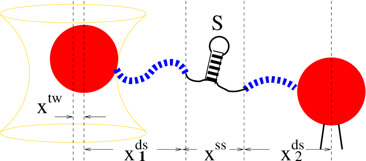
Figure 1:

Figure 2:

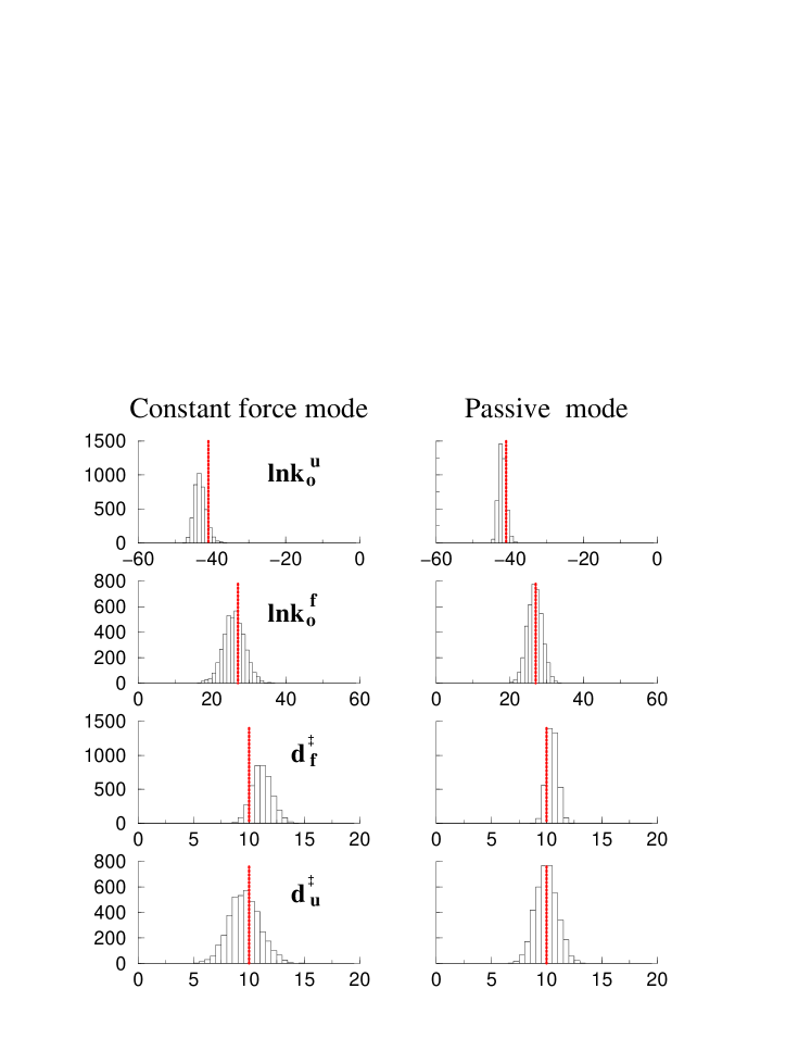
Figure 3:

References

- (1) J.B. Liphardt, et al., Science 292, 733 (2001).
- (2) M.T. Woodside, et al., Science 314, 1001 (2006).
- (3) J.D. Wen, et al., Biophys. J. 92, 2996 (2007).
- (4) M. Manosas et al., Biophys. J. 92, 3010 (2007).
- (5) M. Manosas and F. Ritort, Biophys. J. 88, 3224 (2005).
- (6) J.F. Marko and E.D. Siggia, Macromolecules, 28, 8759 (1995).
- (7) C. Bustamante, J.F. Marko, E.D. Siggia, and S. Smith, Science 264, 1599 (1994).
- (8) We do not need to model the handles and ssRNA chain independently, because the effective persistent length of a sequence of connected worm like chains (WLCs) can be calculated by the following formula: , where and (i=1,,n) are the contour lengthes and persistent lengthes of the WLCs, respectively. (Chen and Yan, personal communications).
- (9) G.I. Bell, Science 200, 618 (1978).
- (10) M. Dembo, et al., Proc. R. Soc. Lond. B Biol. Sci. 234, 55 (1988).
- (11) E. Evans and K. Ritchie, Biophys. J. 72, 1541 (1997).
- (12) B.E. Shapiro and H. Qian, Biophys. Chem. 67, 211 (1997).
- (13) O.K. Dudko, G. Hummer and A. Szabo Phys. Rev. Lett. 96, 108101 (2006).
- (14) It has been known that as force increases, the transtion state location in any one-dimensional potential necessarily decreases and thus weakens the dependence of the unfolding rate on the force Dudkoprl . A cutoff of the rate here can be seen as very rough approximation to this procedure. Of course, we can replace this rate by other rate formulas having microscopic foundation, which would be left in the analysis of real single-molecule data.
- (15) Another extreme case, the slow diffusion limiting () is not of interest in theory and experiment for the distance of of the centers of the beads does not change with time.
- (16) L.R. Rabiner, Proc. IEEE 77, 257 (1989).
- (17) A. Gelman, J.B. Carlin, H.S. Stern, and D.B. Rubin, Bayesian Data Analysis (Chapman and Hall, 1995).