Electroweak Model Without A Higgs Particle

Abstract

An electroweak model is formulated in a finite, four-dimensional quantum field theory without a Higgs particle. The W and Z masses are induced from the electroweak symmetry breaking of one-loop vacuum polarization graphs. The theory contains only the observed particle spectrum of the standard model. In terms of the observed twelve lepton and quark masses, a loop calculation of the non-local electroweak energy scale $\Lambda_{W}$ and $\rho$ predicts the values $\Lambda_{W}(M_{Z})=541$ GeV and $\rho(M_{Z})=0.993$, yielding $s^{2}_{Z}\equiv\sin^{2}\theta_{W}(M_{Z})=0.21686\pm 0.00097$. Possible ways to detect a non-local signal in scattering amplitudes involving loop graphs at the LHC are discussed. Fermion masses are generated from a “mass gap” equation obtained from the lowest order, finite fermion self-energy with a broken symmetry vacuum state. The cross section for $W_{L}^{+}W_{L}^{-}\rightarrow W_{L}^{+}W_{L}^{-}$ is predicted to vanish for $\sqrt{s}>{1\,\rm TeV}$, avoiding a violation of the unitarity bound. The Brookhaven National Laboratory measurement of the anomalous magnetic moment of the muon and the residual difference between the measured value and the standard model can provide a test of a non-local deviation from the standard model.
e-mail: john.moffat@utoronto.ca

I Introduction

Although the standard model has been remarkably successful, as of 2007 no experiment has directly detected the existence of the Higgs boson. After more than forty years of particle physics, we are faced with the fundamental question: What breaks electroweak symmetry? The answer is expected to be provided by the Large Hadron Collider (LHC) at CERN, which will begin operations in 2008.

The Higgs field in vacuum acquires a non-zero value with a constant vacuum expectation value equal to $246$ GeV, which spontaneously breaks the electroweak gauge symmetry $SU(2)\times U(1)$ Higgs . The Higgs mechanism gives mass to the gauge bosons and to the observed leptons and quarks in the standard model Halzen ; Burgess . The non-observation of clear signals leads to an experimental lower bound for the Higgs mass of $114.4$ GeV at 95% confidence level. The standard model does not predict the Higgs mass but if the mass is between 115 and 180 GeV, then the standard model can remain valid up to the Planck energy scale $\sim 10^{16}$ TeV. It is expected from theoretical arguments that the highest possible mass allowed for the Higgs boson is around $\sim\,0.8-1$ TeV. Supersymmetry models predict that the lightest Higgs boson of several such bosons should have a mass around 120 GeV. The LEP Working Group predicts the Higgs mass to be around $m_{H}\sim 144$ GeV based on precision electroweak data, non-observation of the Higgs today and the hypothesis that the minimal standard model is correct CERN . It is expected that the LHC will be able to confirm or deny the existence of the Higgs particle.

In the following, an electroweak model based on a finite gauge field theory Moffat ; Moffat2 ; Moffat3 ; Moffat4 ; Moffat5 begins with an initially $SU(2)_{L}\times U(1)_{Y}$ gauge invariant and massless theory for free non-interacting particles. Then a finite, non-local interaction possessing an extended gauge symmetry with the infinite-dimensional gauge group $G(NL,4)$ makes the theory finite to all orders of perturbation theory Moffat5 ; Hand ; Woodard ; Kleppe ; Hand2 ; Cornish ; Cornish2 ; Cornish3 ; Woodard2 ; Clayton ; Paris ; Troost ; Joglekar ; Moffat6 ; Moffat7 . A dynamical electroweak symmetry breaking measure in the path integral breaks the $G(NL,4)$ gauge symmetry. The symmetry breaking mechanism allows the $W$ and $Z$ gauge bosons to acquire masses through the lowest order vacuum polarization graphs containing fermion loops, while the photon remains massless. The tree graphs are identical to the standard model, excluding the Higgs particle and they are strictly local, maintaining classical locality and macroscopic causality. The non-local effects in the theory occur only in quantum loops and vanish as $\hbar\rightarrow 0$. An experimental signature for the model is that the cross section for $W^{+}_{L}W^{-}_{L}\rightarrow W^{+}_{L}W^{-}_{L}$ ($W_{L}$ denotes the longitudinal part of the massive intermediate vector boson $W$) vanishes above $\sim\,1$ TeV avoiding a violation of the unitarity bound. Thus, the W and Z bosons become massless as the measure becomes the $G(NL,4)$ gauge invariant measure above $\sim\,1$ TeV, and only the transverse components of the W and Z bosons survive.

An important signature for discovering the origin of electroweak symmetry breaking is the observation at the LHC of $WW$ scattering. The vanishing of the $W_{L}W_{L}\rightarrow W_{L}W_{L}$ scattering cross section above $\sim\,1$ TeV would be a signature for a no-Higgs particle, ultra-violet finite quantum field theory. On the other hand, if the cross section is observed to be strong above $\sim\,1$ TeV, then it is saying that possible new strong interactions and the exchange of new intermediary particles are responsible for the electroweak symmetry breaking. If the Higgs particle is observed at the LHC, then the $W_{L}W_{L}$ scattering will not be strong, but at the same time it will not be expected to vanish above $\sim\,1$ TeV.

The masses of fermions are generated through the mass-gap equation obtained from the lowest order finite, fermion-boson self-energy graph with a broken symmetry vacuum state. The spectrum of particles only contains the observed $W$, $Z$ and photon particles and the standard quarks and leptons.

The electroweak model based on a finite quantum field theory (FQFT) without a Higgs particle avoids the fine-tuning (hierarchy) problem associated with the Higgs scalar field radiative corrections. A calculation of the $\rho$ parameter from the finite boson-fermion self-energy loop graphs yields the predictions for the weak mixing angle, $\sin^{2}\theta_{W}(M_{Z})=0.21686\pm 0.00097$ and the electroweak non-local energy scale $\Lambda_{W}(M_{Z})=541$ GeV. A calculation of the muon $g-2$ anomalous magnetic moment in the FQFT can provide a means for detecting a non-local deviation from the standard model in perturbative loop diagrams.

II Finite Non-Local Electroweak Theory

We shall choose units $c=\hbar=1$ and the metric ${\rm diag}(\eta_{\mu\nu})=(-1,+1,+1,+1)$. The Lagrangian takes the form:

$$L=L_{0}+L_{B}+{\cal L}_{I}+\tilde{\cal L}_{I},$$ (1)

where $L_{0}$ is the local, free kinetic Lagrangian for massless leptons and quarks given by

$$L_{0}=[{\bar{\psi}}^{L}(x)i\gamma\cdot\partial\psi^{L}(x)+{\bar{\psi}}^{R}(x)i\gamma\cdot\partial\psi^{R}(x)],$$ (2)

where $\gamma\cdot\partial=\gamma^{\mu}\partial_{\mu}$. The fields $\psi^{L}(x)$ and $\psi^{R}(x)$ denote local two-component left-handed lepton and quark doublet fields and right-handed lepton and quark singlet fields, respectively, with $\psi^{L}=(1/2)(1-\gamma_{5})\psi$ and $\psi^{R}=(1/2)(1+\gamma_{5})\psi$. The local boson Lagrangian density $L_{B}$ is given by

$$L_{B}=-\frac{1}{4}G^{a\mu\nu}G_{a\mu\nu}-\frac{1}{4}B^{\mu\nu}B_{\mu\nu},$$ (3)

where

$$G^{\mu\nu}_{a}=\partial^{\mu}W^{\nu}_{a}-\partial^{\nu}W^{\mu}_{a}+g\epsilon_{abc}W_{b}^{\mu}W_{c}^{\nu},$$ (4)

and

$$B_{\mu\nu}=\partial_{\mu}B_{\nu}-\partial_{\nu}B_{\mu}.$$ (5)

The $\tilde{\cal L}_{I}$ is an iteratively defined series of higher interactions which strip the non-locality from the tree graphs. The non-local interaction Lagrangian density is described by

$${\cal L}_{I}=-g{\cal J}^{\mu}_{a}(x){\cal W}_{a\mu}(x)-g^{\prime}{\cal J}^{\mu}_{Y}(x){\cal B}_{\mu}(x),$$ (6)

where $g$ and $g^{\prime}$ are electroweak coupling constants. The ${\cal W}_{a\mu}$ and ${\cal B}_{\mu}$ are the non-local gauge boson fields, while the ${\cal J}^{\mu}_{a}$ and ${\cal J}_{Y}$ are the non-local weak isospin and hypercharge currents:

$${\cal J}^{\mu}_{a}(x)=\frac{1}{2}{\bar{\Psi}}^{L}(x)\gamma^{\mu}\tau_{a}\Psi^{L}(x)\quad(a=1,2,3),$$ (7)

and

$${\cal J}^{\mu}_{Y}(x)=-\frac{Y}{2}{\bar{\Psi}}^{L}(x)\gamma^{\mu}\Psi^{L}(x)-\frac{Y}{2}{\bar{\Psi}}^{R}(x)\gamma^{\mu}\Psi^{R}(x),$$ (8)

where $\tau_{a}$ denote the Hermitian Pauli matrices and $Y$ denotes the hypercharge. The $\Psi$ denote the non-local lepton and quark fields in the ${\cal J}^{\mu}_{a}$ and ${\cal J}^{\mu}_{Y}$ currents. In the absence of interactions, ${\cal L}_{I}=0$, the massless Lagrangian is invariant under $SU(2)\times U(1)$ gauge transformations.

The $A_{\mu}$ and $Z_{\mu}$ are linear combinations of the two fields $W_{3\mu}$ and $B_{\mu}$:

$$A_{\mu}=\cos\theta_{W}B_{\mu}+\sin\theta_{W}W_{3\mu},$$ (9)

$$Z_{\mu}=-\sin\theta_{W}B_{\mu}+\cos\theta_{W}W_{3\mu},$$ (10)

where the angle $\theta_{W}$ denotes the weak mixing angle. The electroweak coupling constants $g$ and $g^{\prime}$ are related to the electric charge $e$ by the standard equation

$$g\sin\theta_{W}=g^{\prime}\cos\theta_{W}=e$$ (11)

and we use the standard normalization $\cos\theta_{W}=g/(g^{2}+g^{{}^{\prime}2})^{1/2}$ and $g^{\prime}/g=\tan\theta_{W}$.

The non-local field operators ${\cal W}_{a\mu},{\cal B}_{\mu}$ and $\Psi$ are defined in terms of the local operators $W_{a\mu},B_{\mu}$ and $\psi$ by

$${\cal W}_{a\mu}=\int d^{4}yG(x-y)W_{a\mu}(y)=G\biggl{(}\frac{\partial^{2}}{\Lambda^{2}}\biggr{)}W_{a\mu}(x),$$ (12)

$${\cal B}_{\mu}(x)=\int d^{4}yG(x-y)B_{\mu}(y)=G\biggl{(}\frac{\partial^{2}}{\Lambda^{2}}\biggr{)}B_{\mu}(x),$$ (13)

and

$$\Psi(x)=\int d^{4}yG(x-y)\psi(y)=G\biggl{(}\frac{\partial^{2}}{\Lambda^{2}}\biggr{)}\psi(x).$$ (14)

Here, $\partial^{2}=\partial^{\mu}\partial_{\mu}$ and $G(\partial^{2}/\Lambda^{2})$ is a Lorentz-invariant operator distribution whose momentum space Fourier transform is an entire function. We can write

$$G(x-y)=G\biggl{(}\frac{\partial^{2}}{\Lambda^{2}}\biggr{)}\delta^{4}(x-y),$$ (15)

where $\ell\sim 1/\Lambda$ is a small invariant interval and the high Euclidean momentum damping means that the non-locality has compact support. The Fourier transform of the damping function is defined by

$$\int d^{4}x\exp(ipx)G\biggl{(}\frac{\partial^{2}}{\Lambda^{2}}\biggr{)}=K\biggl{(}-\frac{p^{2}}{\Lambda^{2}}\biggr{)}.$$ (16)

Unitarity conditions require that $K(-p^{2}/\Lambda^{2})$ is an entire function that does not generate new poles on the physical sheet and that the residue of the physical pole remains unity Moffat5 .

The non-local distribution operator is defined by

$$G\biggl{(}\frac{\partial^{2}}{\Lambda_{W}^{2}}\biggr{)}\equiv{\cal E}_{m}=\exp\biggl{(}\frac{\partial^{2}-m^{2}}{2\Lambda_{W}^{2}}\biggr{)},$$ (17)

where $\Lambda_{W}$ denotes the electroweak non-local energy scale. We have

$$\Psi={\cal E}_{0}\psi,\quad\bar{\Psi}={\cal E}_{0}\bar{\psi},$$ (18)

$${\cal W}_{a\mu}={\cal E}_{0}W_{a\mu},\quad{\cal B}_{\mu}={\cal E}_{0}B_{\mu}.$$ (19)

Consider, as an example, the stripping of the non-locality of the tree graphs and the restoration of gauge invariance for the $B_{\mu}$ coupling. We have Moffat5 :

$${\cal L}_{0+1}=-\frac{1}{4}B^{\mu\nu}B_{\mu\nu}-\bar{\psi}i\gamma\cdot\partial\psi+g^{\prime}{\bar{\Psi}}\gamma\cdot{\cal B}\Psi,$$ (20)

where we have for simplicity ignored the left and right-handed structure of the non-local hypercharge current ${\cal J}^{\mu}_{Y}$. Eq.(20) is invariant up to order $g^{{}^{\prime}2}$ under the transformation:

$$\delta B_{\mu}\equiv\delta_{0}B_{\mu}=-\partial_{\mu}\theta,$$ (21)

$$\delta_{1}\psi=ig^{\prime}{\cal E}_{0}{\hat{\theta}\Psi},$$ (22)

where $\hat{\theta}={\cal E}_{0}\theta$. Here, the operator ${\cal E}_{0}$ acts on the product ${\hat{\theta}\Psi}$, while the ${\cal E}_{0}$ in $\hat{\theta}$ acts only upon $\theta$ and the ${\cal E}_{0}$ in $\Psi$ acts only upon $\psi$.

We now form the operator ${\cal O}$:

$${\cal O}\equiv\frac{({\cal E}_{0})^{2}-1}{\partial^{2}}=\int_{0}^{1}\frac{d\tau}{\Lambda_{W}^{2}}\exp\biggl{[}\tau\frac{\partial^{2}}{\Lambda_{W}^{2}}\biggr{]}.$$ (23)

The operator ${\cal O}$ is an entire function of $\partial^{2}$, so it does not produce any poles in the momentum representation that will violate unitarity.

By using the operator ${\cal O}$, we can express the simplest non-local four-point interaction as

$${\cal L}_{2}=-g^{{}^{\prime}2}\bar{\Psi}\gamma\cdot{\cal B}i\gamma\cdot\partial{\cal O}\gamma\cdot{\cal B}\Psi.$$ (24)

The scattering amplitude computed from ${\cal L}_{0+1+2}$ is unchanged from its local point particle antecedent. This comes about because each $V_{2}$ vertex contribution to the amplitude can be split into two terms through decomposing the operator ${\cal O}$ into ${\cal E}_{0}^{2}/\partial^{2}$ and $-1/\partial^{2}$. The first such term cancels the contribution from the corresponding $V_{1}\cdot V_{1}$ channel, while the second term is the local, point particle contribution for that channel. This process can be extended to higher $B_{\mu}$ amplitudes with interactions of the form:

$${\cal L}_{n}=-(-g^{\prime})^{n}\bar{\Psi}\gamma\cdot{\cal B}[i\gamma\cdot\partial{\cal O}\gamma\cdot{\cal B}]^{(n-1)}\Psi.$$ (25)

This sums to give the total $B^{\mu}$ coupling Lagrangian:

$${\cal L}=-\frac{1}{4}B^{\mu\nu}B_{\mu\nu}-\bar{\psi}i\gamma\cdot\partial\psi$$

$$+g^{\prime}\bar{\Psi}\gamma\cdot{\cal B}[1+g^{\prime}i\gamma\cdot\partial{\cal O}\gamma\cdot{\cal B}]^{-1}\Psi.$$ (26)

The extended tree graph scattering amplitude is the same as the local, point particle amplitude and the decoupling of unphysical modes is accomplished. The true amplitudes that differ from the point particle ones contain an internal $B_{\mu}$ line, which are enhanced by an exponential damping factor for each internal momentum.

A modification of the fermionic transformation at each order is

$$\delta_{n}\psi=-i(-g^{\prime})^{n}{\cal E}_{0}\hat{\theta}[i\gamma\cdot\partial{\cal O}\gamma\cdot{\cal B}]^{n-1}\Psi.$$ (27)

Moreover, the sum of all variations gives

$$\delta B_{\mu}=-\partial_{\mu}\theta,$$ (28)

$$\delta\psi=ig^{\prime}{\cal E}_{0}\hat{\theta}[1+g^{\prime}i\gamma\cdot\partial{\cal O}\gamma\cdot{\cal B}]^{-1}\Psi.$$ (29)

It can be proved that $\delta L=0$ at order $g^{{}^{\prime}n}$ establishing the gauge invariance under the non-local gauge transformations Moffat5 .

The non-localization of the interaction Lagrangian has resulted in gauge transformations that mix gauge indices and spinor indices at different spacetime coordinates. The action for the $B_{\mu}$ coupling is invariant under a transformation of the form

$$\delta B_{\mu}(x)=-\partial_{\mu}\theta(x),$$ (30)

$$\delta\psi(x)=ig^{\prime}\int d^{4}yd^{4}z{\cal T}[g^{\prime}B](x,y,z)\theta(y)\psi(z).$$ (31)

Here, ${\cal T}\sim 1+g^{\prime}B+...$ is a representation operator that is a spinorial matrix as well as a functional of the vector field $B_{\mu}$:

$${\cal T}[g^{\prime}B](x,y,z)={\cal E}_{0}[\delta^{4}(x-y)][1+g^{\prime}i\gamma\cdot\partial{\cal O}\gamma\cdot{\cal B}]^{-1}{\cal E}_{0}\delta^{4}(x-z).$$ (32)

The transformations do not form a group, because although the gauge group for the $B_{\mu}$ field is Abelian on shell, it does not close on commutation unless the fermion fields obey their equations of motion:

$$[\delta_{\theta_{1}},\delta_{\theta_{2}}]\psi=-g^{{}^{\prime}2}{\cal E}_{0}\{{\hat{\theta}}_{1}[1+g^{\prime}{\cal B}{\cal O}i\gamma\cdot\partial]^{-1}$$

$$\times i\gamma\cdot\partial{\cal O}{\hat{\theta}}_{2}-(1\longleftrightarrow 2)\}{\cal E}_{0}(i\gamma\cdot\partial+g^{\prime}{\cal E}_{0}\gamma\cdot{\cal B}$$

$$\times[1+g^{\prime}\gamma\cdot{\cal B}{\cal O}i\gamma\cdot\partial]^{-1}{\cal E}_{0})\psi.$$ (33)

However, the transformations are part of an infinite-dimensional group $G(NL,4)$ which includes transformations that vanish in the local limit and only influence the fermi fields.

The non-localization process guarantees gauge invariance to all orders and removes all unphysical couplings to longitudinal vector bosons. It can be extended to the total $W$, $B$ and $\psi$ electroweak Lagrangian. The fact that the tree graphs of the theory are the purely local point-like graphs protects the classical theory from any violation of macroscopic causality. The non-locality resides only in the loop sectors where a violation of micro-causality is potentially hidden by the uncertainty principle. The loop graphs in FQFT are finite to all orders in perturbation theory.

We could equally well have formulated our non-local Lagrangian as

$${\cal L}={\cal L}_{0}+{\cal L}_{B}+L_{I}+{\tilde{L}}_{I},$$ (34)

where now the non-locality is in the free and kinetic energy parts of the Lagrangian and not in the interaction part $L_{I}$. This will place the non-local form factor on the propagators, whereas in the previous process the non-local form factors were imposed on the vertices. Both processes produce a finite, gauge invariant and unitary QFT to all orders in perturbation theory. Another method is to introduce shadow fields and shadow propagators Woodard ; Kleppe ; Woodard2 . This method has been successfully applied to Yang-Mills Lagrangians and to quantum gravity Cornish ; Cornish2 ; Cornish3 ; Woodard2 ; Moffat6 .

We have demonstrated a systematic way of maintaining the gauge invariance of the classically, initially non-local massless Lagrangian which consists of two stages. In the first stage, an $SU(2)\times U(1)$ gauge invariant interaction-free action is made non-local and then an infinite series of chosen higher interactions $\tilde{\cal L}_{I}$ is added to the Lagrangian. These added interactions provide the theory with a new nonlinear and non-local gauge invariance which makes Lorentz invariance compatible with perturbative unitarity at tree order. The second stage consists of finding a measure which makes the functional path integral formalism invariant under the non-local gauge symmetry without destroying perturbative unitarity, namely, by finding a measure whose interactions are entire functions of the derivative operator. This measure then yields a functional formalism which defines a set of Green functions which are ultraviolet finite and Poincaré invariant to all orders, and gives scattering amplitudes which are perturbatively finite. The scattering amplitudes are then analytically continued into the Euclidean momentum space.

III Path Integral Formalism and Measure Factors

The path integral formalism is completed with the expression:

$$\langle T^{*}(O)\rangle=\int[D\bar{\psi}][D\psi][DW][DB]\mu_{\rm inv}O\exp(iS),$$ (35)

where $O$ is a given operator. All the loop graphs are ultraviolet finite and unitary to all orders of perturbation theory for the non-local gauge invariant Lagrangian. In the limit that the non-local weak scale $\Lambda_{W}\rightarrow\infty$, the path integral formalism becomes that of the renormalizable, local point field theory of massless gauge bosons $W$ and $B$.

A determination of measures for fermion loops including all lepton, quark, parity and isospin contributions to vacuum polarization loops has been obtained Moffat3 . For the $W^{\pm}$ sector, the invariant measure for the fermion loops is given by

$$\ln\biggl{(}\mu_{\rm inv}[W^{\pm}]\biggr{)}=ig^{2}\int d^{4}x{\cal W}^{+\mu}{\cal M}_{\mu\nu}[W^{\pm}]{\cal W}^{-\mu},$$ (36)

where

$${\cal M}_{\mu\nu}[W^{\pm}]=\frac{\eta_{\mu\nu}}{(4\pi)^{2}}\sum_{d}C_{d}(L_{1+}(m_{1},m_{2})$$

$$+L_{2+}(m_{1},m_{2})+L_{2+}(m_{2},m_{1})).$$ (37)

Here the sum is over all fermion doublets $d$, and $C_{d}$ denotes the color factors.

The $W^{3\mu}$ and $B^{\mu}$ gauge boson invariant measures for the fermion loop sector are given by

$$\ln\biggl{(}\mu_{\rm inv}[W^{3}]\biggr{)}=\frac{ig^{2}}{2}\int d^{4}x{\cal W}^{3\mu}{\cal M}_{\mu\nu}[W^{3}]{\cal W}^{3\nu},$$ (38)

$${\cal M}_{\mu\nu}[W^{3}]=\frac{\eta_{\mu\nu}}{2(4\pi)^{2}}\sum_{\mathrm{lhf}}C_{f}(L_{1+}(m,m)+2L_{2+}(m,m)),$$ (39)

and

$$\ln\biggl{(}\mu_{\rm inv}[B]\biggr{)}=\frac{ig^{{}^{\prime}2}}{2}\int d^{4}x{\cal B}^{\mu}{\cal M}_{\mu\nu}[B]{\cal B}^{\nu},$$ (40)

$${\cal M}_{\mu\nu}[B]=2\frac{\eta_{\mu\nu}}{(4\pi)^{2}}\biggl{(}\sum_{f}C_{f}\frac{Y_{f}^{2}}{4}(L_{1+}(m,m)$$

$$+2L_{2+}(m,m))+\sum_{\mathrm{rhf}}C_{f}\frac{Y_{L}Y_{R}}{4}(2M_{1}(m)+M_{2}(m))\biggr{)},$$

where $\sum_{\mathrm{lhf}}$ and $\sum_{\mathrm{rhf}}$ denote sums over left-handed and right-handed fermions only, respectively. Moreover, $\sum_{f}=\sum_{\mathrm{rhf}}+\sum_{\mathrm{lhf}}$, $Y_{f}$ denotes the fermion hypercharge factor and $Y_{L}$ and $Y_{R}$ denote the left-handed and right-handed hypercharge factors, respectively. The invariant measure for the off-diagonal $W^{3}-B$ for the fermion loops is

$$\ln\biggl{(}\mu_{\rm inv}[W^{3}-B]\biggr{)}=igg^{\prime}\int d^{4}x{\cal W}^{3\mu}{\cal M}_{\mu\nu}[W^{3}-B]{\cal B}^{\nu},$$ (42)

$${\cal M}_{\mu\nu}[W^{3}-B]=-\frac{\eta_{\mu\nu}}{(4\pi)^{2}}\biggl{(}\frac{1}{2}\sum_{\mathrm{lhf}}C_{f}(L_{1+}(m,m)$$

$$+2L_{2+}(m,m))+\sum_{\mathrm{rhf}}C_{f}\frac{Y_{f}}{2}(M_{1}(m)+M_{2}(m))\biggr{)}.$$

The $Ls$ are given by

$$L_{1\pm}(m_{1},m_{2})=\int^{\infty}_{1}d\tau_{1}\int^{\infty}_{1}d\tau_{2}\exp\biggl{[}-\tau_{1}\frac{m_{1}^{2}}{\Lambda_{W}^{2}}-\tau_{2}\frac{m_{2}^{2}}{\Lambda_{W}^{2}}$$

$$-\frac{\tau_{1}\tau_{2}}{(\tau_{1}+\tau_{2})}\frac{p^{2}}{\Lambda_{W}^{2}}\biggr{]}\biggl{(}\frac{\Lambda^{2}_{W}}{(\tau_{1}+\tau_{2})^{3}}\pm\frac{p^{2}\tau_{1}\tau_{2}}{(\tau_{1}+\tau_{2})^{4}}\biggr{)},$$ (44)

$$L_{2\pm}(m_{1},m_{2})=\int_{0}^{1}d\tau_{1}\int^{\infty}_{1}d\tau_{2}\exp\biggl{[}-\tau_{1}\frac{m_{1}^{2}}{\Lambda_{W}^{2}}-\tau_{2}\frac{m_{2}^{2}}{\Lambda_{W}^{2}}$$

$$-\frac{\tau_{1}\tau_{2}}{(\tau_{1}+\tau_{2})}\frac{p^{2}}{\Lambda_{W}^{2}}\biggr{]}\biggl{(}\frac{\Lambda^{2}_{W}}{(\tau_{1}+\tau_{2})^{3}}\pm\frac{p^{2}\tau_{1}\tau_{2}}{(\tau_{1}+\tau_{2})^{4}}\biggr{)}.$$ (45)

We also have

$$M_{1}=\int^{\infty}_{1}d\tau_{1}\int^{\infty}_{1}d\tau_{2}\frac{m^{2}}{(\tau_{1}+\tau_{2})^{2}}$$

$$\times\exp\biggl{[}-(\tau_{1}+\tau_{2})\frac{m^{2}}{\Lambda_{W}^{2}}-\frac{\tau_{1}\tau_{2}}{(\tau_{1}+\tau_{2})}\frac{p^{2}}{\Lambda_{W}^{2}}\biggr{]},$$ (46)

$$M_{2}=\int^{1}_{0}d\tau_{1}\int^{\infty}_{1}d\tau_{2}\frac{m^{2}}{(\tau_{1}+\tau_{2})^{2}}$$ (47)

$$\times\exp\biggl{[}-(\tau 1+\tau_{2})\frac{m^{2}}{\Lambda_{W}^{2}}-\frac{\tau_{1}\tau_{2}}{(\tau_{1}+\tau_{2})}\frac{p^{2}}{\Lambda_{W}^{2}}\biggr{]}.$$

The transverse, gauge invariant vacuum polarization tensor for the $W$ boson has been determined Moffat2 ; Moffat3 . For the fermion loop sector, we have

$$\Pi_{W}^{\mu\nu}(p^{2})=\Pi_{W}^{T}(p^{2})\biggl{(}\eta^{\mu\nu}-\frac{p^{\mu}p^{\nu}}{p^{2}}\biggr{)}+\Pi_{W}^{L}(p^{2})\frac{p^{\mu}p^{\nu}}{p^{2}},$$ (48)

where $\Pi_{W}^{T}$ and $\Pi_{W}^{L}$ denote the transverse and longitudinal parts, respectively. We obtain $\Pi_{W}$ by adding together the three contributions $\Pi_{W1}$, $\Pi_{W2}$ and $\Pi_{W3}$, where the first term is produced by the standard boson-fermion loop graph, the second by the gauge boson-fermion tadpole graph and the third by the graph associated with the fermion measure factor. The three one-loop vacuum polarization graphs are shown in Figure 1 and Figure 2, and the measure factor graphs are shown in Figure 3.

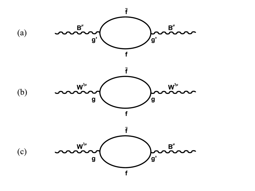
Figure 1: (a) vacuum polarization fermion one-loop graph for the B boson; (b) vacuum polarization fermion one-loop graph for the W boson; (c) the off-diagonal B-W boson fermion one-loop vacuum polarization graph.

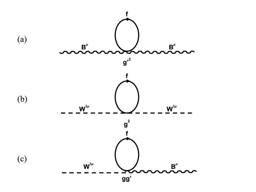
Figure 2: (a) the tadpole fermion one-loop vacuum polarization graph for the B boson; (b) the tadpole fermion one-loop vacuum polarization graph for the W boson; (c) the off-diagonal tadpole fermion W-B boson vacuum polarization graph.

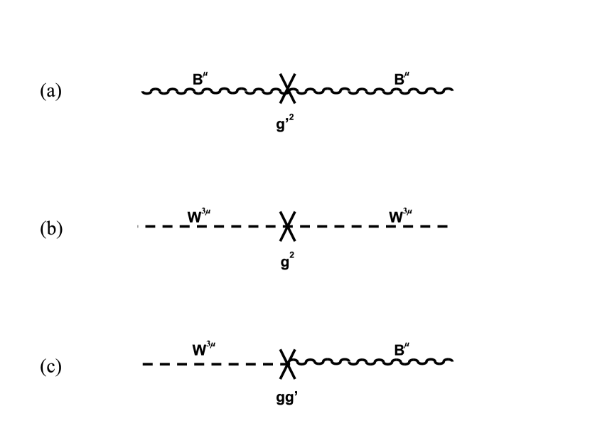
Figure 3: (a) the B boson fermion measure factor contribution; (b) the W boson fermion measure factor contribution; (c) the off-diagonal B-W fermion measure factor contribution.

It can be shown that for the $W^{\pm}$ sector, $\Pi_{W}^{L}=\Pi^{L}_{W1}+\Pi^{L}_{W2}+\Pi^{L}_{W3}=0$ and the transverse part is given by

$$\Pi_{W}^{T}(p^{2})=-\frac{g^{2}}{(4\pi)^{2}}\exp\biggl{(}-\frac{p^{2}}{\Lambda_{W}^{2}}\biggr{)}\sum_{d}C_{d}$$ (49)

$$\times\biggl{(}P_{1}(m_{1},m_{2})+P_{2}(m_{1},m_{2})+P_{2}(m_{2},m_{1})\biggr{)}.$$

The $Ps$ are given by

$$P_{1}=L_{1+}-L_{1-}=2p^{2}\int^{\infty}_{1}d\tau_{1}\int^{\infty}_{1}d\tau_{2}$$

$$\times\exp\biggl{[}-\tau_{1}\frac{m_{1}^{2}}{\Lambda_{W}^{2}}-\tau_{2}\frac{m_{2}}{\Lambda_{W}^{2}}-\frac{\tau_{1}\tau_{2}}{\tau_{1}+\tau_{2}}\frac{p^{2}}{\Lambda_{W}^{2}}\biggr{]}\frac{\tau_{1}\tau_{2}}{(\tau_{1}+\tau_{2})^{4}},$$

and

$$P_{2}=L_{2+}-L_{2-}=2p^{2}\int^{1}_{0}d\tau_{1}\int^{\infty}_{1}d\tau_{2}$$

$$\times\exp\biggl{[}-\tau_{1}\frac{m_{1}^{2}}{\Lambda_{W}^{2}}-\tau_{2}\frac{m_{2}}{\Lambda_{W}^{2}}-\frac{\tau_{1}\tau_{2}}{\tau_{1}+\tau_{2}}\frac{p^{2}}{\Lambda_{W}^{2}}\biggr{]}\frac{\tau_{1}\tau_{2}}{(\tau_{1}+\tau_{2})^{4}}.$$

We observe that $P_{1}$ and $P_{2}$ are proportional to $p^{2}$, so they vanish as $p^{2}\rightarrow 0$ guaranteeing that $\Pi^{T}(0)=0$ and keeping the gauge bosons $W$ and $Z$ massless.

The measures for the invariant pure Yang-Mills boson loops can be determined. For example, the $B^{\mu}$ measure is given by

$$\ln\biggl{(}\mu_{\rm inv}[B]\biggr{)}=-ig^{{}^{\prime}2}\int d^{4}x{\cal B}^{\mu}{\cal M}[B]{\cal B}_{\mu},$$ (52)

where

$${\cal M}[B]=\frac{\Lambda_{W}^{2}}{2^{4}\pi^{2}}\int^{1}_{0}\frac{d\tau}{(\tau+1)^{2}}\exp\biggl{(}-\frac{\tau}{(\tau+1)}\frac{p^{2}}{\Lambda_{W}^{2}}\biggr{)}$$

$$\times\biggl{(}\frac{2}{\tau+1}-3+6\frac{\tau}{\tau+1}\biggr{)}.$$ (53)

IV Dynamical Symmetry Breaking

We must now introduce a method to generate the physical $W$ and $Z$ gauge boson masses. This will be achieved by dynamically breaking the electroweak non-local gauge symmetry by an appropriate choice of the fermion sector measure, so that $\Pi(m_{\rm phys}^{2})\not=0$ and a mass is induced at $p^{2}=-m_{\rm phys}^{2}$, making the $W$ and $B$ particles massive vector bosons.

To lowest order, we find that the $W$ boson propagator is modified according to

$$D_{W\alpha\beta}(p)\rightarrow D_{W\alpha\beta}(p)+D_{W\alpha\mu}(p)g^{2}\Pi_{W}^{\mu\nu}(p^{2})D_{W\nu\beta}(p).$$ (54)

We now have that

$$\frac{-\eta_{\alpha\beta}}{p^{2}-i\epsilon}\rightarrow\frac{-\eta_{\alpha\beta}}{p^{2}-i\epsilon}+\frac{\eta_{\alpha\mu}}{p^{2}-i\epsilon}g^{2}\Pi^{\mu\nu}_{W}(p^{2})\frac{\eta_{\nu\beta}}{p^{2}-i\epsilon}.$$ (55)

It follows that

$$\frac{1}{p^{2}-i\epsilon}\rightarrow\frac{1}{p^{2}-i\epsilon}-\frac{1}{p^{2}-i\epsilon}g^{2}\Pi_{W}(p^{2})\frac{1}{p^{2}-i\epsilon},$$ (56)

where

$$v\equiv\Pi_{W}(p^{2})=\frac{1}{4}{\Pi_{W}^{\mu}}_{\mu}(p^{2}).$$ (57)

To lowest order we get

$$\frac{1}{p^{2}-i\epsilon}\rightarrow\frac{1}{p^{2}+g^{2}\Pi_{W}(p^{2})-i\epsilon}+O(g^{4}),$$ (58)

where in our regularized theory $\Pi_{W}(p^{2})$ is finite. The mass is defined on the mass shell to be

$$m^{2}_{\rm phys}=g^{2}\Pi(m^{2}_{\rm phys}).$$ (59)

The symmetry breaking measure is defined by

$$\ln\biggl{(}\mu_{SB}\biggr{)}=-igg^{\prime}\int d^{4}x{\cal W}^{3\mu}\biggl{(}{\cal M}_{\mu\nu}[W^{3}-B]\biggr{)}_{SB}{\cal B}^{\nu}$$

$$+\frac{ig^{{}^{\prime}2}}{2}\int d^{4}x{\cal B}^{\mu}\biggl{(}{\cal M}_{\mu\nu}[B]\biggr{)}_{SB}{\cal B}^{\nu},$$ (60)

where

$$\biggl{(}{\cal M}_{\mu\nu}[W^{3}-B]\biggr{)}_{SB}=$$

$$-\frac{\eta_{\mu\nu}}{(4\pi)^{2}}\sum_{\mathrm{rhf}}C_{f}\frac{Y_{f}}{2}(M_{1}(m)+M_{2}(m)),$$ (61)

and

$$\biggl{(}{\cal M}_{\mu\nu}[B]\biggr{)}_{SB}=\frac{2\eta_{\mu\nu}}{(4\pi)^{2}}\biggl{\{}\sum_{\mathrm{rhf}}C_{f}\bigg{[}\frac{Y_{f}^{2}}{4}(L_{1+}(m,m)$$

$$+2L_{2+}(m,m))+\frac{Y_{L}Y_{R}}{4}(2M_{1}(m)+M_{2}(m))\biggr{]}$$

$$+\sum_{\mathrm{lhf}}C_{f}\biggl{(}\frac{Y_{f}^{2}-1}{4}\biggr{)}(L_{1+}(m,m)+2L_{2+}(m,m))\biggr{\}}.$$

The vacuum polarization tensor $\Pi^{\mu\nu}(W^{3})$ for the $W^{3}$ sector is given by

$$\Pi^{\mu\nu}(W^{3})=\frac{g^{2}}{2(4\pi)^{2}}\exp\biggl{(}-\frac{p^{2}}{\Lambda_{W}^{2}}\biggr{)}\sum_{\mathrm{lhf}}C_{f}\biggl{[}(L_{1+}(m,m)$$

$$+2L_{2+}(m,m))\biggl{(}\eta^{\mu\nu}-\frac{p^{\mu}p^{\nu}}{p^{2}}\biggr{)}$$

$$+(L_{1-}(m,m)+2L_{2-}(m,m))\frac{p^{\mu}p^{\nu}}{p^{2}}\biggr{]}.$$ (63)

For the $W^{\pm}$ sector we have

$$\Pi^{\mu\nu}(W^{\pm})=\frac{g^{2}}{2(4\pi)^{2}}\exp\biggr{(}-\frac{p^{2}}{\Lambda_{W}^{2}}\biggr{)}\sum_{d}C_{d}\biggl{[}(L_{1+}(m_{1},m_{2})$$

$$+L_{2+}(m_{1},m_{2})+L_{2+}(m_{2},m_{1}))\biggl{(}\eta^{\mu\nu}-\frac{p^{\mu}p^{\nu}}{p^{2}}\biggr{)}$$

$$+(L_{1-}(m_{1},m_{2})+L_{2-}(m_{1},m_{2})+L_{2-}(m_{2},m_{1}))\frac{p^{\mu}p^{\nu}}{p^{2}}\biggr{]}.$$

(64)

We get for the $B$ and $W^{3}-B$ sectors

$$\Pi^{\mu\nu}(B)=\frac{g^{{}^{\prime}2}}{2(4\pi)^{2}}\exp\biggl{(}-\frac{p^{2}}{\Lambda_{W}^{2}}\biggr{)}\sum_{\mathrm{lhf}}C_{f}$$

$$\times\biggl{[}(L_{1+}(m,m)+2L_{2+}(m,m))\biggl{(}\eta^{\mu\nu}-\frac{p^{\mu}p^{\nu}}{p^{2}}\biggr{)}$$

$$+(L_{1-}(m,m)+2L_{2-}(m,m))\frac{p^{\mu}p^{\nu}}{p^{2}}\biggr{]},$$ (65)

and

$$\Pi^{\mu\nu}(W^{3}-B)=-\frac{gg^{\prime}}{2(4\pi)^{2}}\exp\biggl{(}-\frac{p^{2}}{\Lambda_{W}^{2}}\biggr{)}\sum_{\mathrm{lhf}}C_{f}$$

$$\times\biggl{[}(L_{1+}(m,m)+2L_{2+}(m,m))\biggl{(}\eta^{\mu\nu}-\frac{p^{\mu}p^{\nu}}{p^{2}}\biggr{)}$$

$$+(L_{1-}(m,m)+2L_{2-}(m,m))\frac{p^{\mu}p^{\nu}}{p^{2}}\biggr{]}.$$ (66)

The measure $\mu_{SB}$ dynamically breaks the non-local gauge invariance and the $W$ and $B$ gauge bosons acquire a finite mass. The relative strength of the neutral and charged current interactions is fixed by means of the standard relation:

$$\rho\frac{G_{F}}{\sqrt{2}}=\frac{g^{2}}{8M_{Z}^{2}\cos^{2}\theta_{W}},$$ (67)

where $G_{F}$ is the Fermi constant and $G_{F}/\sqrt{2}=g^{2}/8M_{W}^{2}$. We obtain from (67) the standard result:

$$\rho=\frac{M_{W}^{2}}{M_{Z}^{2}\cos^{2}\theta_{W}}.$$ (68)

The Lagrangian picks up a finite mass contribution for $\rho=1$ from the total sum of polarization graphs:

$$L_{M}=\frac{1}{8}v^{2}g^{2}[(W^{1}_{\mu})^{2}+(W^{2}_{\mu})^{2}]$$ (69)

$$+\frac{1}{8}v^{2}[g^{2}(W^{3}_{\mu})^{2}-2gg^{\prime}W^{3}_{\mu}B^{\mu}+g^{{}^{\prime}2}B^{2}_{\mu}]$$

$$=\frac{1}{4}g^{2}v^{2}W^{+}_{\mu}W^{-\mu}$$

$$+\frac{1}{8}v^{2}(W_{3\mu},B_{\mu})\left(\begin{matrix}g^{2}&-gg^{\prime}\\ -gg^{\prime}&g^{{}^{\prime}2}\end{matrix}\right)\left(\begin{matrix}W^{3\mu}\\ B^{\mu}\end{matrix}\right),$$

where $W^{\pm}_{\mu}=(W^{1}\mp iW^{2})/\sqrt{2}$ and we can fix the value of $v$ from $G_{F}/\sqrt{2}=g^{2}/8M_{W}^{2}$ to be $v=246$ GeV. We see that we have the usual dynamical symmetry breaking mass matrix in which one of the eigenvalues of the $2\times 2$ matrix in (69) is zero. From (9) and (10), we get for $\rho=1$:

$$M_{W}=\frac{1}{2}vg,\quad M_{Z}=\frac{1}{2}v(g^{2}+g^{{}^{\prime}2})^{1/2},\quad M_{A}=0.$$ (70)

V Evaluation of $\rho$ and $\Lambda_{W}$

We shall now calculate $\rho$ and $\Lambda_{W}$ from the loop diagrams for non-zero lepton and quark masses, $m_{f}\not=0$. We obtain for $\rho$ the result:

$$\rho=2\sum_{i}C_{i}d_{i}[L_{1}(p^{2},m_{dbi1},m_{dbi2})$$ (71)

$$+L_{2}(p^{2},m_{dbi1},m_{dbi2})+L_{2}(p^{2},m_{dbi2},m_{dbi1})]$$

$$\times\{\sum_{i}C_{i}f_{i}[L_{1}(p^{2},m_{fi})+2L_{2}(p^{2},m_{fi})]\}^{-1}.$$

Using $M_{W}=(1/2)vg$, we can obtain an equation that can be solved for the electroweak energy scale $\Lambda_{W}$:

$$v=\frac{1}{4\pi}\{\exp(-p^{2}/\Lambda_{W}^{2})4\sum_{i}C_{i}d_{i}[L_{1}(p^{2},m_{dbi1},m_{dbi2})$$

$$+L_{2}(p^{2},m_{dbi1},m_{dbi2})+L_{2}(p^{2},m_{dbi2},m_{dbi1})]\}^{1/2}.$$

The $m_{dbi}$ denote the fermion doublets: $[e,\nu_{e}],[\mu,\nu_{\mu}],[\tau,\nu_{\tau}],[d,u],[s,c],[b,t]$, and the color factors are $C_{\ell}=1$ for leptons and $C_{q}=3$ for quarks.

The quantities that enter the calculations of $\rho$ and $\Lambda_{W}$ are obtained from the traces of (63) and (64). We have

$$L_{1}=\frac{1}{4}(3L_{1+}+L_{1-}),\quad L_{2}=\frac{1}{4}(3L_{2+}+L_{2-}).$$ (73)

The $Ls$ are given by

$$L_{1\pm}(p^{2},m_{1},m_{2})$$

$$=\int^{\infty}_{1}d\tau_{1}\int^{\infty}_{1}d\tau_{2}\exp\biggl{[}-\frac{\tau_{1}m_{1}^{2}+\tau_{2}m_{2}^{2}}{\Lambda_{W}^{2}}-\frac{\tau_{1}\tau_{2}p^{2}}{(\tau_{1}+\tau_{2})\Lambda_{W}^{2}}\biggr{]}$$

$$\times\biggl{(}\frac{\Lambda_{W}^{2}}{(\tau_{1}+\tau_{2})^{3}}\pm\frac{p^{2}\tau_{1}\tau_{2}}{(\tau_{1}+\tau_{2})^{4}}\biggr{)},$$ (74)

$$L_{2\pm}(p^{2},m_{1},m_{2})$$

$$=\int^{1}_{0}d\tau_{1}\int^{\infty}_{1}d\tau_{2}\exp\biggl{[}-\frac{\tau_{1}m_{1}^{2}+\tau_{2}m_{2}^{2}}{\Lambda_{W}^{2}}-\frac{\tau_{1}\tau_{2}p^{2}}{(\tau_{1}+\tau_{2})\Lambda_{W}^{2}}\biggr{]}$$

$$\times\biggl{(}\frac{\Lambda_{W}^{2}}{(\tau_{1}+\tau_{2})^{3}}\pm\frac{p^{2}\tau_{1}\tau_{2}}{(\tau_{1}+\tau_{2})^{4}}\biggr{)}.$$ (75)

In the calculation of $\Lambda_{W}$ and $\rho$, we include the six observed lepton masses pdg :

$$m_{e}=0.000511\,{\rm GeV},\,m_{\mu}=0.10566\,{\rm GeV},$$

$$m_{\tau}=1.777\pm 0.025\,{\rm GeV},\,m_{\nu_{e}}=0.2\times 10^{-8}\pm 0.09\,{\rm GeV},$$

$$m_{\nu_{\mu}}=0.00019\pm 0.07\,{\rm GeV},\,m_{\nu_{\tau}}=0.0182\pm 1.8\,{\rm GeV},$$

and the six observed quark masses pdg ; Tevatron :

$$m_{u}=0.0019\,{\rm GeV},\,m_{d}=0.0044\,{\rm GeV},$$

$$m_{s}=0.095\pm 0.025\,{\rm GeV},\,m_{c}=1.31\pm 0.09\,{\rm GeV},$$

$$m_{b}=4.24\pm 0.07\,{\rm GeV},\,m_{t}=170.9\pm 1.8\,{\rm GeV}.$$ (77)

From (71), it follows that for $m_{f}=0$ we get $\rho=1$ and for $m_{t}\rightarrow\infty$ we obtain $\rho=0.857$. The former result corresponds to the tree graph value obtained from the standard model and yields the prediction:

$$s_{Z}^{2}\equiv\sin^{2}\theta_{W}(M_{Z})=0.22239\pm 0.00095.$$ (78)

In the calculations of $\rho$ and $\Lambda_{W}$ the top quark mass $m_{t}$ dominates the calculations.

We obtain from (LABEL:Lambda) the non-local energy scale at the Euclidean on shell value $p^{2}=M_{Z}^{2}$:

$$\Lambda_{W}(M_{Z})=541\,{\rm GeV},$$ (79)

and for $\rho$ at the Z-pole, we get from (71):

$$\rho(M_{Z})=0.993.$$ (80)

The experimental values of the $W$ and $Z$ boson masses are given by Tevatron ; pdg :

$$M_{W}=80.413\pm 0.029\,{\rm GeV},\,M_{Z}=91.1876\pm 0.0021\,{\rm GeV}.$$ (81)

This predicts from (68) and (80) the value

$$s_{Z}^{2}\equiv\sin^{2}\theta_{W}(M_{Z})=0.21686\pm 0.00097.$$ (82)

A calculation in the standard model including radiative corrections gives the value pdg :

$$s_{Z}^{2}=0.23122\pm 0.00015.$$ (83)

A more accurate prediction of $s_{Z}^{2}$ in our non-local QFT requires calculating further radiative corrections in our electroweak model. A calculation of the $\rho$ and $\Lambda_{W}$ at $p^{2}=0$ yields values close to (79) and (82) calculated at the $Z$-pole.

VI Fermion Masses

In the standard electroweak model, fermion masses are generated through Yukawa couplings $\langle\phi\rangle\bar{\psi}\psi$ where $\langle\phi\rangle$ is the vacuum expectation value of the Higgs field $\phi$. In our model, we shall generate fermion masses from the finite one-loop fermion self-energy graph by means of a Nambu-Jona-Lasinio mechanism Nambu . The one-loop fermion self-energy graphs are shown in Figure 4. A fermion particle will satisfy

$$i\gamma\cdot p+m_{0f}+\Sigma(p)=0,$$ (84)

for $i\gamma\cdot p+m_{f}=0$ where $m_{0f}$ is the bare fermion mass, $m_{f}$ is the observed fermion mass and $\Sigma(p)$ is the finite proper self-energy part. We have

$$m_{f}-m_{0f}=\Sigma(p,m_{f},g,\Lambda_{f})|_{i\gamma\cdot p+m_{f}=0}.$$ (85)

Here, $\Lambda_{f}$ denote the non-local energy scales for lepton and quark masses. We can solve (84) and (85) by successive approximations starting from the bare mass $m_{0f}$. However, we can also find solutions for $m_{f}\not=0$ when $m_{0f}=0$ for a broken symmetry vacuum state.

The finite self-energy contribution obtained by joining together two fermion-boson vertices is given by Moffat5 :

$$-i\Sigma_{1}(p)=\int\frac{d^{4}k}{(2\pi)^{2}}(ig^{2}_{f}\gamma^{\mu})\biggl{(}\frac{-i}{\gamma\cdot\partial+m_{f}-i\epsilon}\biggr{)}(ig^{2}_{f}\gamma^{\nu})$$ (86)

$$\times\biggl{(}\frac{-i\eta_{\mu\nu}}{k^{2}+m^{2}-i\epsilon}\biggr{)}$$

$$\times\exp\biggl{[}-\biggl{(}\frac{p^{2}+m_{f}^{2}}{\Lambda_{f}^{2}}\biggr{)}-\biggl{(}\frac{q^{2}+m_{f}^{2}}{\Lambda_{f}^{2}}\biggr{)}-\frac{k^{2}}{\Lambda_{f}^{2}}\biggr{]},$$

where $g^{2}_{f}$ is a fermion coupling constant which contains quark color factors, $q=p-k$ and we choose the boson zero mass limit. The propagators are now converted to Schwinger integrals and the momentum integration is performed to give

$$-i\Sigma_{1}(p)=-g^{2}_{f}\exp\biggl{[}-\biggl{(}\frac{p^{2}+m_{f}^{2}}{\Lambda_{f}^{2}}\biggr{)}\biggr{]}$$ (87)

$$\times\int^{\infty}_{1}\frac{d\tau_{1}}{\Lambda_{f}^{2}}\int^{\infty}_{1}\frac{d\tau_{2}}{\Lambda_{f}^{2}}\int\frac{d^{4}k}{(2\pi)^{4}}(2\gamma\cdot q+4m_{f})$$

$$\times\exp\biggl{[}-\tau_{1}\biggl{(}\frac{q^{2}+m^{2}}{\Lambda_{f}^{2}}\biggr{)}-\tau_{2}\frac{k^{2}}{\Lambda_{f}^{2}}\biggr{]}$$

$$=\frac{-ig_{f}^{2}}{8\pi^{2}}\exp\biggl{[}-\biggl{(}\frac{p^{2}+m_{f}^{2}}{\Lambda_{f}^{2}}\biggr{)}\biggr{]}$$

$$\times\int^{\infty}_{1}d\tau_{1}\int^{\infty}_{1}d\tau_{2}\biggl{[}\frac{\tau_{2}}{(\tau_{1}+\tau_{2})^{3}}\gamma\cdot p+\frac{2m_{f}}{(\tau_{1}+\tau_{2})^{2}}\biggr{]}$$

$$\times\exp\biggl{(}-\frac{\tau_{1}\tau_{2}}{\tau_{1}+\tau_{2}}\frac{p^{2}}{\Lambda_{f}^{2}}-\tau_{1}\frac{m_{f}^{2}}{\Lambda_{f}^{2}}\biggr{)}.$$

Here, we have performed a rotation to Euclidean momentum space, accounting for the factor of $i$.

Another contribution $\Sigma_{2}(p)$ to the self-energy comes from the tadpole fermion-boson self-energy graph:

$$-i\Sigma_{2}(p)=\int\frac{d^{4}k}{(2\pi)^{2}}(-ig_{f}^{2})\gamma^{\mu}(\gamma\cdot q-m_{f})\gamma^{\nu}\biggl{(}\frac{-i\eta_{\mu\nu}}{k^{2}-i\epsilon}\biggr{)}$$

$$\times\int_{0}^{1}\frac{d\tau}{\Lambda_{f}^{2}}\exp\biggl{[}-\biggl{(}\frac{p^{2}+m_{f}^{2}}{\Lambda_{f}^{2}}\biggr{)}-\tau\biggl{(}\frac{q^{2}+m_{f}^{2}}{\Lambda_{f}^{2}}\biggr{)}-\frac{k^{2}}{\Lambda_{f}^{2}}\biggr{]}.$$

Adding together the two diagram contributions $\Sigma_{1}(p)$ and $\Sigma_{2}(p)$, we obtain

$$\Sigma(p)=\frac{g^{2}_{f}}{8\pi^{2}}\exp\biggl{[}-\biggl{(}\frac{p^{2}+m_{f}^{2}}{\Lambda_{f}^{2}}\biggr{)}\biggr{]}$$

$$\times\int^{1}_{0}dx(x\gamma\cdot p+2m_{f})E_{1}\biggl{[}(1-x)\frac{p^{2}}{\Lambda^{2}_{f}}+\biggl{(}\frac{1-x}{x}\biggr{)}\frac{m_{f}^{2}}{\Lambda_{f}^{2}}\biggr{]}.$$

Here, $E_{1}$ is the exponential integral:

$$E_{1}(z)\equiv\int^{\infty}_{z}dy\frac{\exp(-y)}{y}$$ (90)

$$=-\ln(z)-\gamma_{e}-\sum^{\infty}_{n=1}\frac{(-z)^{n}}{nn!},$$

where $\gamma_{e}$ is Euler’s constant. By developing an asymptotic expansion in $\Lambda_{f}$ and expanding the exponential integral, we get

$$\Sigma(p)=\frac{\alpha_{f}}{2\pi}\biggl{[}\biggl{(}\frac{1}{2}\gamma\cdot\partial p+2m_{f}\biggr{)}\ln(\Lambda_{f}^{2})$$ (91)

$$-\biggl{(}\frac{1}{2}\gamma\cdot\partial p+2m_{f}\biggr{)}\gamma_{e}+\frac{1}{2}\gamma\cdot\partial p$$

$$-\int^{1}_{0}dx(x\gamma\cdot\partial p+2m_{f})\ln(xp^{2}+m_{f}^{2})$$

$$+O\biggl{[}\frac{\ln(\Lambda^{2}_{f})}{\Lambda_{f}^{2}}\biggr{]},$$

where $\alpha_{f}=g^{2}_{f}/4\pi$.

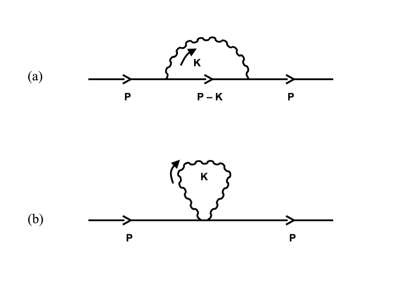
Figure 4: (a) the one-loop fermion self-energy graph; (b) the fermion one-loop self-energy tadpole graph.

The fermion mass is now identified with $\Sigma(p)$ at $p=0$:

$$m_{f}=\Sigma(0)=\frac{\alpha_{f}m_{f}}{\pi}\biggl{[}\ln\biggl{(}\frac{\Lambda_{f}^{2}}{m_{f}^{2}}\biggr{)}-\gamma_{e}\biggr{]}+O\biggl{[}\frac{\ln(\Lambda^{2}_{f})}{\Lambda_{f}^{2}}\biggr{]}.$$ (92)

This equation has two solutions: either $m_{f}=0$, or

$$1=\frac{\alpha_{f}}{\pi}\biggl{[}\ln\biggl{(}\frac{\Lambda_{f}^{2}}{m_{f}^{2}}\biggr{)}-\gamma_{e}\biggr{]}.$$ (93)

The first trivial solution corresponds to the standard perturbation result. The second non-trivial solution will determine $m_{f}$ in terms of $\alpha_{f}$ and $\Lambda_{f}$ and leads to the fermion “mass gap” equation

$$m_{f}=\Lambda_{f}\exp\biggl{[}-\frac{1}{2}\biggl{(}\frac{\pi}{\alpha_{f}}+\gamma_{e}\biggr{)}\biggr{]}.$$ (94)

The non-perturbative solution for the fermion masses is based on a broken vacuum state with $\langle{\bar{\psi}\psi}\rangle_{0}\not=0$ and avoids introducing bare fermion masses in the $SU(2)\times U(1)$ gauge invariant zero mass and zero interaction limit. The Lagrangian picks up fermion mass terms:

$$L_{M_{f}}=m_{f}{\bar{\psi}}_{f}\psi_{f}$$ (95)

$$= m_{f}\psi_{f}[\frac{1}{2}(1-\gamma_{5})+\frac{1}{2}(1+\gamma_{5})]\psi_{f}$$

$$= m_{f}({\bar{\psi}}^{R}\psi^{L}+{\bar{\psi}}^{L}\psi^{R}).$$

By choosing $\alpha_{f}=\alpha_{s}(M_{Z})=0.117\pm 0.0007$, where $\alpha_{s}$ is the strong coupling constant evaluated at the $m_{Z}$ pole, and $\Lambda_{t}=1.55\times 10^{5}\,{\rm TeV}$, we find for the top quark mass, $m_{t}=171\,{\rm GeV}$.

VII Unitarity and the Scale of $W_{L}W_{L}$ Scattering

We can separate the Lagrangian into a gauge invariant sector and a symmetry breaking sector

$${\cal L}={\cal L}_{\rm gauge\,inv}+{\cal L}_{\rm SB}.$$ (96)

Here, ${\cal L}_{\rm gauge\,inv}$ possesses the unbroken $G(NL,4)$ gauge symmetry with massless, transversely polarized gauge bosons $W,Z$ and $\gamma$. ${\cal L}_{\rm SB}$ describes the dynamical symmetry breaking. In the standard model, the Higgs mechanism ensures that the three Goldstone bosons, $w^{\pm}$ and $z$, couple to the three gauge currents associated with the spontaneously broken symmetry of $SU(2)_{L}\times U(1)_{Y}$. At the same time, it ensures that $w^{\pm}$ and $z$ become longitudinal modes of the gauge bosons $W^{\pm}$ and $Z$, which become massive independently of whether the Higgs boson exists or not.

A rigorous bound on the energy dependence of $W_{L}W_{L}$ scattering comes from unitarity. If we set $\rho=1$, then the $I=J=0$ partial wave amplitude is given by

$$A_{00}(W_{L}W_{L})=\frac{s}{16\pi v^{2}},$$ (97)

where $s$ is the square of the center-of-mass energy. Unitarity demands that below 4-body thresholds $A_{00}\leq 1$, and $Re(A_{00})\leq 1/2$. Both of these conditions are violated above 1.8 and 1.2 TeV, respectively Chanowitz .

For $s\ <<M^{2}_{\rm SB}$, where $M_{\rm SB}$ is the typical symmetry breaking mass scale of ${\cal L}_{\rm SB}$, we get the amplitude:

$${\cal A}(W^{+}_{L}W^{-}_{L}\rightarrow Z_{L}Z_{L})=\frac{1}{\rho}\frac{s}{v^{2}},$$ (98)

in the energy range $M_{W}^{2}\ll s\ll M^{2}_{\rm SB}$. For leading order in the unitary-gauge the amplitude in the gauge sector yields the behavior:

$${\cal A}(W^{+}_{L}W^{-}_{L}\rightarrow Z_{L}Z_{L})_{\rm gauge\,sector}$$

$$=\frac{g^{2}s}{4\rho M_{W}^{2}}+O(g^{2}s^{0})\sim\frac{s}{\rho v^{2}}.$$ (99)

This high energy behavior eventually violates unitarity and the standard local QFT theory without a Higgs particle is non-renormalizable. The inclusion of a Higgs exchange at the scale $M_{\rm SB}$ cancels the “bad” high energy behavior and allows unitarity to be satisfied above $\sim\,1$ TeV and the theory is renormalizable. In particular, the low energy behavior for $s\ll M^{2}_{\rm SB}$ can be shown to decouple the ${\cal L}_{\rm SB}$ to all orders.

For our finite non-local electroweak theory, we require that ${\cal A}(W^{+}_{L}W^{-}_{L}\rightarrow Z_{L}Z_{L})$ vanishes above $\sim\,1$ TeV, avoiding the unitarity violating behavior of the standard gauge sector with massive vector bosons $W$ and $Z$. We implement this by requiring that the symmetry breaking fermion loop measure becomes the gauge invariant measure, $\mu_{\rm SB}\rightarrow\mu_{\rm inv}$, above $\sim\,1$ TeV. Thus, the $W$ and $Z$ bosons become massless gauge bosons above $\sim\,1$ TeV with only transverse polarization degrees of freedom and there is no violation of unitarity. The massless boson, non-local gauge invariant theory becomes the standard local renormalizable theory when $\Lambda_{W}\rightarrow\infty$. The signature of a vanishing cross section for $W_{L}^{+}W_{L}^{-}$ scattering above $\sim\,1$ TeV should be detectable at the LHC.

In the non-local QFT with a finite non-local scale $\Lambda_{W}$, the partial wave scattering amplitude $A_{\ell}(s,t)$ (where $t$ is the momentum transfer squared) for the crossed channel in lowest order scattering diagrams will behave badly at high energies. A similar phenomenon occurs in perturbative string theory Gross . To circumvent this problem, it is necessary to re-sum the scattering amplitudes to arbitrary order in perturbation theory. In QFT the on-shell high energy behavior of scattering amplitudes poses difficult questions, for it combines both short and long distance physics. The fixed $t$, large $s$ behavior of QCD reveals this problem even for the case of fixed angle scattering. For FQFT the exact leading behavior of the scattering amplitude has to be deduced, order by order in perturbation theory, by means of a saddle point calculation. The exponential behavior of string theory scattering amplitudes is unlike the power behavior that holds in QFT. The same is true of the finite loop graphs in non-local QFT. In contrast to perturbative string theory, the FQFT tree graphs behave at high energies as in local, point particle QFT. However, the lowest order behavior of the crossed channel amplitudes in non-local QFT violates the rigorous bound of Cerulus and Martin Martin , which states that $|A(s,\cos\theta)|\geq\exp[-\sqrt{s}\ln s\,c(\theta)]$. The proof of this bound uses unitarity, a finite mass threshold gap and the assumption of a polynomial bound in the energy for fixed $t$ of the scattering amplitudes. The polynomial behavior of scattering amplitudes in standard QFT is a consequence of locality. The non-local QFT like string theory manages to be sufficiently non-local to avoid a polynomial bound, yet maintains sufficiently local interactions to preserve causality.

VIII Experimental Signatures of Non-local Electroweak Theory

We have seen that at $\sqrt{s}\sim\,0.5-1$ TeV the non-local scale $\Lambda_{W}$ becomes significant corresponding to an exponential fall-off of the loop scattering amplitudes in the s-channel. The tree graph scattering amplitudes at large energies are strictly local and have the same high energy behavior as in the standard point QFT. A detection of a non-local behavior in the loop scattering amplitudes at the LHC at $\sqrt{s}>0.5-1$ TeV would be an experimental confirmation of non-local QFT. This could be observed in a different high energy behavior of scattering amplitudes involving loop diagrams in, say, photon-proton Compton scattering.

In the standard electroweak model, the quadratic divergence of the Higgs mass radiative correction is a serious problem and has motivated several alternative models beyond the standard model. In the Higgs potential:

$$V(\phi)=-\frac{1}{2}\mu^{2}\phi^{2}+\frac{1}{4}\lambda\phi^{4},$$ (100)

the mass parameter $\mu^{2}$ at tree level ($\mu^{2}>0$ for spontaneous symmetry breaking) is related to the vacuum expectation value $v$ by $\mu^{2}=\lambda v^{2}$. When radiative corrections are calculated, the mass parameter becomes $\mu_{0}^{2}+\delta\mu^{2}$, where $\mu_{0}^{2}$ is the bare mass term and $\delta\mu^{2}$ is the radiative correction. Since the radiative correction depends on the cutoff scale as $\Lambda_{C}^{2}$, the fine-tuning between the bare mass term and the radiative correction becomes significant for $\Lambda_{C}>1$ TeV. If the cutoff reaches the Planck energy scale, then the amount of fine-tuning is enormous and a tuning of order $10^{32}$ is needed. This is the source of the naturalness or hierachy problem in standard electroweak theory. Because our FQFT does not possess a Higgs particle, the Higgs fine-tuning problem does not occur.

Because the $W$, $Z$ and $\gamma$ tree graphs in FQFT electroweak theory are identical to those of the standard electroweak theory, all the lower energy predictions of the standard model at tree graph level remain the same when the Higgs particle graphs are excluded. One probe of the FQFT is the calculated difference between the experimental and local, standard model theoretical values of the muon $a_{\mu}=(g-2)/2$ anomaly. The Brookhaven National Laboratory experiment has determined $a_{\mu}$ with a much improved accuracy BNL . The experimental value is: $(a_{\mu})_{\rm exp}=1165208.0(6.3)\times 10^{-10}$. The difference between this result and the standard model prediction $(a_{\mu})_{\mathrm{SM}}$ is: $(22.4\pm 10)\times 10^{-10}\leq\delta a_{\mu}\leq(26.1\pm 9.4)\times 10^{-10}$.

We obtain the bound on a possible non-local QFT contribution for the anomalous magnetic moment of the muon:

$$\delta(a_{\mu})_{\rm nl}\leq\frac{K}{\Lambda_{W}^{2}}.$$ (101)

From (101) and from our estimated value for the electroweak non-local scale $\Lambda_{W}(M_{Z})=541$ GeV, we get the bound:

$$K\leq 701\pm 338\,({\rm MeV})^{2}.$$ (102)

Thus, a careful calculation of the non-local contribution to $a_{\mu}$ could test the prediction of FQFT.

IX Conclusions

We have constructed an electroweak model based on a method to make a massless gauge invariant QFT into a non-local theory which is finite, Poincaré invariant, and perturbatively unitary. The method has two stages – classical and quantum. In the first we make the theory finite by non-localizing its interactions. The violation of unphysical decoupling is then removed at each order by adding an appropriate new interaction. The resulting tree graphs decouple from unphysical modes and the action possesses a generalized gauge invariance in the form of the non-local group $G(NL,4)$. In the electroweak theory, the new symmetry can be viewed on shell as a non-local and non-linear representation of $SU(2)\times U(1)$.

The quantum stage of our method consists of finding measures to make the functional formalism invariant, and then to find a path integral measure that dynamically breaks the non-local gauge symmetry to give the $W$ and $Z$ bosons mass while keeping the photon massless. We have also proposed a method for giving leptons and quarks mass through a mass gap equation. This is done directly through the finite fermion self-energy radiative diagram in terms of a fermion mass scale $\Lambda_{f}$.

The number of unknown parameters in our extended electroweak theory is reduced by not having an unpredictable Higgs mass but we have a new predicted energy scale parameter $\Lambda_{W}$. The number of fermion mass scale parameters $\Lambda_{f}$ – one for each observed lepton and quark – is the same as occurs in the standard Higgs Yukawa coupling model. This number of undetermined parameters still points to the need for a more comprehensive unified theory of the particle interactions, which would determine the unknown parameters in a fundamental way.

The nice feature of our extended electroweak theory is that it does not increase the number of particles, nor does it extend the number of dimensions as in string theory, yet it preserves Poincaré invariance and a finite electroweak theory.

We have proposed ways to test our FQFT. The vanishing of the cross section for $W^{+}_{L}W^{-}_{L}\rightarrow W^{+}_{L}W^{-}_{L}$ above $\sim\,1$ TeV should be observable at the LHC. Moreover, the behavior of scattering amplitudes for, say, Compton proton-photon scattering above $\Lambda_{W}\sim 0.5-1$ TeV is another way to detect the non-local behavior of finite loop graphs. We have also shown that a calculation of the non-local loop contribution to the muon anomalous $g-2$ magnetic moment $a_{\mu}$ could reveal the difference between FQFT with $\Lambda_{W}\sim 0.5$ TeV and the standard model calculation of $a_{\mu}$.

If the Tevatron and LHC accelerator experiments fail to detect a Higgs particle, then a physically consistent theory of electroweak symmetry breaking such as the one studied here, in which no Higgs particle is included in the particle spectrum, will be required to understand the important phenomenon of how the $W$ and $Z$ bosons and fermions acquire mass.

Acknowledgements: I thank Clifford Burgess and Martin Green for stimulating discussions. I also thank Viktor Toth for stimulating discussions and valuable suggestions for obtaining and checking numerical results. This research was supported by a grant from NSERC. The Perimeter Institute is supported in part by the Government of Canada through NSERC and by the Province of Ontario through MEDT.

References

• (1) P. Higgs, Phys. Lett. 12, 132 (1964); P. Higgs, Phys. Rev. Lett. 13, 508 (1964); F. Englert and R. Brout, Phys. Rev. Lett. 13, 321 (1964); P. Higgs, Phys. Rev. 145, 1156 (1966).
• (2) F. Halzen and A. D. Martin, Quarks and Leptons: An Introductory Course in Modern Particle Physics, John Wiley & Sons. 1984.
• (3) C. P. Burgess and G. D. Moore, The Standard Model: A Primer, Cambridge University Press, 2007.
• (4) The LEP Electroweak Working Group, http://lepewwg.web.cern.ch
• (5) J. W. Moffat, Phys. Rev. D41, 1177 (1990).
• (6) J. W. Moffat, Mod. Phys. Lett. 6, 1011 (1991).
• (7) M. Clayton and J. W. Moffat, Mod. Phys. Lett. 6, 2697 (1991).
• (8) J. W. Moffat, Phys. Rev. D39, 3654 (1989).
• (9) D. Evens, J. W. Moffat, G. Kleppe and R. P. Woodard, Phys. Rev. D43, 499 (1991).
• (10) J. W. Moffat and S. M. Robbins, Mod. Phys. Lett. A6, 1581 (1991).
• (11) B. J. Hand and J. W. Moffat, Phys. Rev. D43, 1896 (1991).
• (12) G. Kleppe and R. P. Woodard, Phys. Lett. B253, 331 (1991).
• (13) G. Kleppe and R. P. Woodard, Nucl. Phys. B388, 81 (1992).
• (14) B. J. Hand, Phys. Lett. B275, 419 (1992).
• (15) N. J. Cornish, Mod. Phys. Lett. 7, 631 (1992).
• (16) N. J. Cornish, Mod. Phys. Lett. 7, 1895 (1992).
• (17) N. J. Cornish, Int. J. Mod. Phys. A 7, 6121 (1992).
• (18) G. Kleppe and R. P. Woodard, Ann. of Phys. 221, 106 (1993).
• (19) M. A. Clayton, L. Demopolous and J. W. Moffat, Int. J. Mod. Phys. A9, 4549 (1994).
• (20) J. Paris, Nucl. Phys. B450, 357 (1995).
• (21) J. Paris and W. Troost, Nucl. Phys. B482. 373 (1996).
• (22) G. Saini and S. D. Joglekar, Z. Phys. C76, 343 (1997).
• (23) J. W. Moffat, arXiv: hep-ph/0003171 v2; arXiv: hep-ph/0102088 v2.
• (24) Tevatron Electroweak Working Group (http://tevewwg.fnal.gov/top/).
• (25) W.-M. Yao, et al., Review of Particle Physics, J. of Phys., (http://pdg.lbl.gov.)
• (26) Y. Nambu and G. Jona-Lasinio, Phys. Rev. 122, 345 (1961).
• (27) M. S. Chanowitz, Czech. J. Phys. 55, B45 (2005), ArXiv: hep-ph/0412203.
• (28) D. J. Gross and P. F. Mende, Phys. Lett. B197, 129 (1987).
• (29) F. Cerulus and A. Martin, Phys. Lett. 8, 80 (1963).
• (30) G. W. Bennett et al., Phys. Rev. D73 072003 (2006).