Coherence lifetimes of excitations in an atomic condensate due to the thin spectrum

Abstract

We study the quantum coherence properties of a finite sized atomic condensate using a toy-model and the thin spectrum model formalism. The decoherence time for a condensate in the ground state, nominally taken as a variational symmetry breaking state, is investigated for both zero and finite temperatures. We also consider the lifetimes for Bogoliubov quasi-particle excitations, and contrast them to the observability window determined by the ground state coherence time. The lifetimes are shown to exhibit a general characteristic dependence on the temperature, determined by the thin spectrum accompanying the spontaneous symmetry breaking ground state.

I INTRODUCTION

Although the first observation of superfluid behavior in helium-4 dates back to 1937 superfluid , it was not until 1995 that superfluid associated with Bose-Einstein condensation (BEC) bec_original was discovered in dilute atomic gases bec95 . While the atom-atom interactions are too complicated to handle in liquid state helium-4, a dilute atomic gas opens the possibility to construct a microscopic theory for superfluidity. Since 1995, atomic quantum gases have served as excellent fertile ground for studying quantum coherence properties of matter and for testing interesting many body theories.

The theoretical and experimental studies of atomic condensates have also focused on their quantum coherence properties. Shortly after the initial discovery of BEC, it was understood that a finite sized condensate, in addition to the usual decoherence due to imperfect isolation from the environment, suffers from quantum phase diffusion walls ; you96 , an interaction driven decoherence due to atomic number fluctuations from within the condensate hansch . This study suggests a third source of decoherence, which we show limits the lifetime of a quasi-particle excitation from a condensate, based on the mechanism of thin spectrum as recently proposed and applied to any quantum system with a spontaneously broken symmetry wezel06 ; wezel05 ; wezel07 . Our work therefore constitutes a natural application of the thin spectrum formalism to the highly successful mean field theory for atomic condensates, where the condensate is treated as a U(1) gauge symmetry breaking field.

This paper is organized as follows: we begin with a review of a toy model calculation for the lifetime of the coherent condensate ground state as well as a squeezed ground state and a thermal coherent state. We then review the concept of thin spectrum and show how it is connected with spontaneous symmetry breaking and decoherence of an atomic condensate. In sec. IV, we show how the quasi-particle excitations of an atomic Bose-Einstein condensate are affected by the thin spectrum associated with the ground state condensate. Finally, in sec. V we show how to generalize the idea of thin spectrum to systems with multiple broken symmetries. Concluding remarks are provided in sec. VI.

II a toy model

The basic idea of dephasing from the ground state phase collapse can be understood based on the ’zero-mode’ dynamics of a toy model toy1 ; toy2 . The ground state of an $N$ boson system is with all $N$ bosons in the lowest energy eigenstate, the zero momentum state for a homogeneous gas. However, it cannot simply be a Fock state since Bose-Einstein condensation entails a definite phase from the broken phase U(1) symmetry, while a number state has no definite phase. A reasonable approximation is to consider a coherent state occupation for the zero-mode with an amplitude $\alpha=\sqrt{N}$. Taking $\alpha$ real is equivalent to explicitly picking a phase of the U(1) symmetry. Because such a coherent state is not an energy eigenstate, it suffers phase collapse walls ; you96 . In this section, we discuss the dynamics of the associated phase collapse based on a simple toy model to calculate the rate of this collapse and study the modifications arising from a squeezed ground state.

II.1 The lifetime for the coherent ground state

We discuss the zero mode due to BEC, which results in the breaking the $U(1)$ gauge symmetric Hamiltonian

$$\mathcal{H}=\frac{\tilde{u}}{2}\hat{a}^{\dagger}\hat{a}^{\dagger}\hat{a}\hat{a}-\mu\hat{a}^{\dagger}\hat{a},$$ (1)

where $\hat{a}$ denotes the atomic annihilation operator for the condensate (zero) mode. $\tilde{u}$ scales as $\tilde{u}=u_{0}/V$ with $V$ the quantization volume and $u_{0}$ the effective interaction constant defined as $u_{0}=4\pi a_{s}\hbar^{2}/M$. $a_{s}$ is the s-wave scattering length and $M$ is the atomic mass. $\mu$ is the chemical potential, a Lagrange multiplier for fixing the density of the average number of condensed particles $N$ in the quantization volume $V$. We consider a variational, symmetry breaking ground state, a coherent state satisfying $\hat{a}|z\rangle=z|z\rangle$. Such a state can be formally generated by the displacement operator $D(z)=\exp(z\hat{a}-z^{*}\hat{a}^{\dagger})$ acting on the vacuum state, or $D(z)|0\rangle=|z\rangle$. Minimization of the mean free energy $\langle z|\mathcal{H}|z\rangle$ then fixes $|z|\simeq\sqrt{N}$. This coherent state can be expanded in terms of the eigenvectors of the Hamiltonian, e.g. the Fock number states $|n\rangle$ so that

$$|z\rangle={\rm e}^{-|z|^{2}/2}\sum_{n=0}^{\infty}\frac{z^{n}}{\sqrt{n!}}|n\rangle.$$ (2)

In this case the order parameter for BEC, is the expectation value of the annihilation operator. In the Heisenberg picture, the operator $\hat{a}(t)$ is

$$\hat{a}(t)={\rm e}^{\frac{i}{\hbar}\mathcal{H}t}\hat{a}\,{\rm e}^{-\frac{i}{\hbar}\mathcal{H}t}.$$ (3)

In terms of the eigenenergy $E_{n}=\frac{\tilde{u}}{2}(n^{2}-n)-\mu n$, defined through $\mathcal{H}|n\rangle=E_{n}|n\rangle$, for the $n$-th Fock state $|n\rangle$, one can easily calculate

$$\langle z|\hat{a}|z\rangle = \sqrt{N}\exp\left(N[{\rm e}^{-\frac{i}{\hbar}\tilde{u}t}-1]\right){\rm e}^{\frac{i}{\hbar}\mu t},$$ (4)

whose short time behavior is found to be

$$\langle z|\hat{a}|z\rangle=\sqrt{N}{\rm e}^{\frac{i}{\hbar}\mu t}{\rm e}^{-i\frac{N\tilde{u}}{\hbar}t}{\rm e}^{-\frac{N\tilde{u}^{2}}{2\hbar^{2}}t^{2}},$$ (5)

i.e., revealing an exponential decay walls ; you96 . At longer time scale, it turns out that $\langle z|\hat{a}|z\rangle$ revives due to the discrete, and thus periodic, nature of the exact time evolution (4).

The short time decay defines a collapse-time proportional to $t_{c}\sim\hbar/\sqrt{N}\tilde{u}$. The ratio of the revival time $t_{r}$ required for the order parameter scales as $t_{r}/t_{c}=\sqrt{N}$, and becomes infinite in the thermodynamic limit. In order to get an estimate of this $t_{c}$, we introduce a characteristic length scale for the harmonic trap potential as $a_{\rm ho}=\sqrt{\hbar/(M\omega_{\rm tr})}$, in terms of the harmonic trap frequency $\omega_{\rm tr}$. Denoting the density of condensed atom numbers in the quantization volume as $\rho=N/V$, we find

$$t_{c}=\frac{\sqrt{N}}{4\pi N_{\rm eff}}\frac{1}{\omega_{\rm tr}},$$ (6)

where we have defined $N_{\rm eff}=\rho a_{\rm ho}^{2}a_{s}$. Assuming a typical situation of current experiments with $N\sim 10^{6}$, $a_{s}=10$ nm, $a_{\rm ho}=1$ $\mu$m, and $\rho=10^{21}$ m^-3, we get $t_{c}\simeq 10/\omega_{\rm tr}$. For a magnetic trap with $\omega_{\rm tr}=100$ Hz, this amounts to $t_{c}\sim 10^{-1}$ seconds, clearly within the regime to be confirmed and studied experimentally hansch .

II.2 A squeezed ground state

The unitary squeezing operator mandel for a single bosonic mode is defined as

$$S(\gamma)={\rm e}^{\frac{\gamma}{2}\hat{a}\hat{a}-\frac{\gamma^{*}}{2}\hat{a}^{\dagger}\hat{a}^{\dagger}}.$$ (7)

The squeezed coherent state $|\alpha,\gamma\rangle=D(\alpha)S(\gamma)|vac\rangle$ is also a minimum uncertainty state, although its fluctuations in the two orthogonal quadratures are not generally equal to each other. Fluctuations of one quadrature are reduced or squeezed at the expense of the other. The arguments of $\gamma$ and $\alpha$ determine which quadrature is squeezed. In particular, if both $\gamma$ and $\alpha$ are real, then the state is a number squeezed state, with the uncertainty in atom number reduced at the cost of higher uncertainty in the conjugate phase variable. We expect such a state to have a longer life time, since the phase collapse speed is generally proportional to $\Delta N$, which is smaller in this case, as have recently observed experimentally mara ; ibloch . A wide phase distribution, on the other hand, makes the squeezed state more similar to a Fock state which has a uniform phase distribution, and is less influenced by the decoherence effect due to the U(1) symmetry breaking field because of the reduced number fluctuations.

In order to understand the essence of the above discussion, we choose to follow similar arguments as with the coherent state considered previously. We will study the time evolution of the single mode state $|\alpha,\gamma\rangle$ subject to the same $U(1)$ gauge symmetric Hamiltonian (1). For notational convenience we define

$$\zeta=\gamma\frac{\tanh(|\gamma|)}{|\gamma|}.$$ (8)

The Fock state expansion of the squeezed state in terms of this new variable is wunsche

$$|\alpha,\gamma\rangle = \sum_{n=0}^{\infty}A_{n}(\alpha,\zeta)|n\rangle$$ (9)

$$= (1-|\zeta|^{2})^{1/4}{\rm e}^{-\frac{(\alpha+\zeta\alpha^{*})\alpha^{*}}{2}}$$

$$\sum_{n=0}^{\infty}\sqrt{\frac{\zeta^{n}}{2^{n}n!}}H_{n}\left(\frac{\alpha+\zeta\alpha^{*}}{\sqrt{2\zeta}}\right)|n\rangle,$$

where $H_{n}$ is the n-th order Hermite polynomial. In the limit $x\rightarrow\infty$, $H_{n}(x)$ behaves like $2^{n}x^{n}$. Hence, the squeezed state approaches a coherent state when $\zeta\rightarrow 0$. The corresponding expectation value for $\hat{a}(t)$ now takes the form

$$\langle\alpha,\gamma|\hat{a}(t)|\alpha,\gamma\rangle=\sum_{n=0}^{\infty}\sqrt{n+1}A_{n}^{*}A_{n+1}{\rm e}^{\frac{i}{\hbar}(E_{n}-E_{n+1})t},$$ (10)

where the complex nature of $A_{n}(\alpha,\zeta)$ makes the analytic evaluation of this expression nontrivial. We therefore resort to numerical studies. In a recent paper, number squeezing of the initial state by a factor of $10$ was reported mara . This corresponds to $\gamma=\ln{10}$ or $\zeta\simeq 0.98$. In our numerical calculations, we consider the time evolution of (10) for $\alpha=10$ at $\zeta=0.5$ and $0.9$. The results in Fig. 1 manifest that squeezing in the particle number fluctuations improves the coherence time for the condensate. The phase space distributions of the initial states used in Fig. 1 are displayed in Fig. 2. The longest lived preparation of the condensate is the one with strongest squeezing in the particle number or the one with largest phase fluctuations. In order to examine how the phase distribution evolves in time, we can look the propagation of the Q-function. We find that all coherent preparations of the condensate eventually lose the imprinted phase information, and the system recovers its uniform phase distribution as in a Fock state. A typical result of our simulations is presented in Fig. 3. By initially preparing the condensate in a number squeezed coherent state, with already broad phase distribution, longer life times of the condensate are achieved.

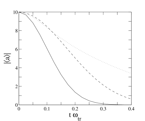
Figure 1: The comparison of the short time decay character for a coherent state condensate with that for a squeezed state at $\zeta=0.5$ and $\zeta=0.9$. The parameters used are $a_{s}=10$ nm, $a_{\rm ho}=1$ $\mu$m, $n=10^{21}$ m^-3, but now for $N=100$. In this case, the dimensionless time in units of $\hbar/\tilde{u}$ becomes $\hbar/\tilde{u}=\omega_{\rm tr}^{-1}$. The fastest decay (solid line) denotes the result for a coherent state, while the dashed (dotted) line refers to that of a squeezed state with $\zeta=0.5$ ($\zeta=0.9$). As expected, the choice of a squeezed state with real parameters $\alpha$ and $\zeta$ improves the coherence time.

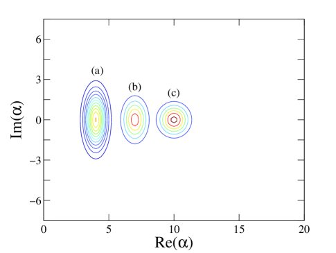
Figure 2: (Color online) The phase space distributions of the initial states used in Fig. 1. Curves (a), (b) and (c) correspond to $\zeta=0.9$, $\zeta=0.5$ and $\zeta=0$, respectively. Although all of them should be centered at $\alpha=10$, they are shifted for convenience.

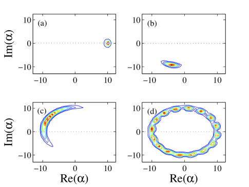
Figure 3: (Color online) Time evolution of the Q-function for a squeezed-coherent state with $\alpha=10$ and $\zeta=0.5$ for different values of $t\omega_{tr}$. Figures (a), (b), (c) and (d) shows the Q-function distributions for $t\omega_{tr}=0$, $t\omega_{tr}=0.02$, $t\omega_{tr}=0.10$ and $t\omega_{tr}=0.40$. It is seen that as the order parameter decays, the broken phase symmetry is restored, since the Q-function distribution becomes rotationally symmetric.

More generally, our discussions can reach beyond the choices of real parameters $\alpha$ and $\zeta$. Consequently, different results may be expected, as we illustrate the comparisons between a coherent state and squeezed states with $\zeta=0.5$, $\zeta=0.5i$, and $\zeta=-0.5$ in Fig. 4. We see that the last two choices of the squeezing parameters lead to reduced coherence times, a result that again can be reasonably understood in terms of the increased uncertainty in the atom number, as it causes faster collapse.

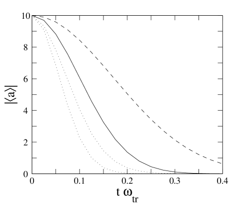
Figure 4: Decay of the order parameter for the coherent state and squeezed states of $\zeta=0.5$, $\zeta=0.5i$ and $\zeta=-0.5$ as a function of $t\omega_{tr}$. The solid line is the coherent state, the dashed line is the squeezed state with $\zeta=0.5$, and the dotted ones are the squeezed states with $\zeta=0.5i$ and $\zeta=-0.5$. Only the state with real squeezing parameter has a longer life time than the coherent state.

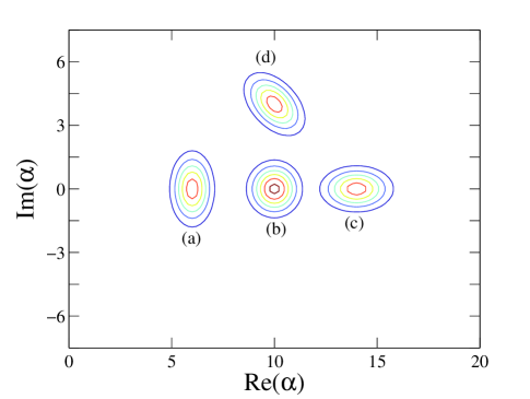
Figure 5: (Color online) The phase space distributions of the initial states used in Fig. 4. Curves (a), (b), (c) and (d) correspond to $\zeta=0.5$, $\zeta=0$, $\zeta=-0.5$ and $\zeta=0.5i$, respectively. Although all of them should be centered at $\alpha=10$, they are shifted for convenience.

II.3 A thermal coherent state

To extend the above discussions to finite temperature systems, we will now introduce the thermal coherent state, which possesses both a thermal character as well as a phase. Consider the following density matrix for a thermal state

$$\rho_{\rm th} = {\rm e}^{-\beta\mathcal{H}}$$ (11)

$$= \sum_{n}{\rm e}^{-\beta E_{n}}|n\rangle\langle n|,$$

where $\beta=1/k_{B}T$, $k_{B}$ is the Boltzmann constant and $T$ is the temperature. In this state (11), $\mathcal{H}$ is the Hamiltonian operator, $\mathcal{H}=\tilde{u}\hat{a}^{\dagger}\hat{a}^{\dagger}\hat{a}\hat{a}/2$. $E_{n}$ is redefined, corresponding to $\mathcal{H}|n\rangle=E_{n}|n\rangle$. $\rho_{\rm th}$ is a mixed state that has a thermal character but not a definite phase. In order to introduce a coherent component, and also to change the mean number of atoms, we can make use of the displacement operator

$$\rho=D(\alpha)\rho_{\rm th}D^{\dagger}(\alpha).$$ (12)

We shall call this state a thermal coherent state, whose properties can be conveniently studied with the aid of the generalized coherent or displaced number states roy82

$$D(\alpha)|n\rangle = |n,\alpha\rangle$$ (13)

$$= \sum_{n=0}^{\infty}{\rm e}^{-\frac{1}{2}|\alpha|^{2}}\sqrt{\frac{n!}{m!}}\alpha^{m-n}\text{L}_{n}^{m-n}(|\alpha|^{2})|m\rangle\hskip 24.0pt$$

$$= \sum_{n=0}^{\infty}C_{m}(n,\alpha)|m\rangle,$$

where $L_{k}^{l}$ is the generalized Laguerre Polynomial. The thermal coherent density matrix now becomes

$$\rho = \sum_{n=0}^{\infty}{\rm e}^{-\beta E_{n}}D(\alpha)|n\rangle\langle n|D^{\dagger}(\alpha)$$ (14)

$$= \sum_{n=0}^{\infty}{\rm e}^{-\beta E_{n}}|n,\alpha\rangle\langle n,\alpha|$$

$$= \sum_{nmm^{\prime}}{\rm e}^{-\beta E_{n}}C_{m}(n,\alpha)C_{m^{\prime}}^{*}(n,\alpha)|m\rangle\langle m^{\prime}|,$$

with which we can again consider the time evolution of the expectation value of $\hat{a}(t)$,

$$\langle\hat{a}(t)\rangle = \sum_{nmm^{\prime}k}{\rm e}^{-\beta E_{n}}C_{m}(n,\alpha)C_{m^{\prime}}^{\dagger}(n,\alpha)\langle k|m\rangle$$ (15)

$$\langle m^{\prime}|{\rm e}^{\frac{i}{\hbar}\mathcal{H}t}\hat{a}{\rm e}^{-\frac{i}{\hbar}\mathcal{H}t}|k\rangle,$$

calculated according to $\langle\hat{a}(t)\rangle=\text{Tr}\left(\rho\hat{a}(t)\right)$. In the end, we find

$$\langle\hat{a}(t)\rangle = \sum_{nm}{\rm e}^{-\beta E_{n}}C_{m+1}(n,\alpha)C_{m}^{*}(n,\alpha)$$ (16)

$$\sqrt{m}\,{\rm e}^{-\frac{i}{\hbar}(E_{m+1}-E_{m})t}.$$

In general, the phase factors will interfere destructively in the above. The thermal distribution weight ${\rm e}^{-\beta E_{n}}$ term determines how many different terms contribute. This implies that the temperature definitely leads to a reduced coherence time for the state. For the initial preparations of a condensate of $100$ atoms, as depicted in Fig. 5, Fig. 6 illustrates the decay of these condensates at various temperatures.

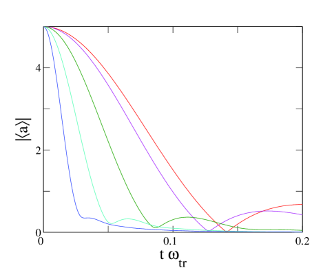
Figure 6: (Color online) The short time decays for thermal coherent states. The lines correspond respectively to $T=1000$ nK, 100 nK, 10 nK, 1 nK, and 0.001 nK from left to right. The humps are entirely due to the ground degeneracy $E_{0}=E_{1}$. Even as the temperature approaches zero, the state (12) does not approach the ordinary coherent state $D(\alpha)|0\rangle$. Instead, it is a superposition state $D(\alpha)(|0\rangle+|1\rangle)/\sqrt{2}$.

III The thin spectrum formalism

III.1 A simple theory

By the thin spectrum, we typically refer to a group of states whose energy spacings are so low that they are not exactly controllable in any experiments. The effect of such states on the partition function and on the decoherence has been studied extensively, for instance see Ref. wezel06 . In many-body systems, models of thin spectra arise quite often whenever there exists a spectrum with level spacing inversely proportional to the system size. These states with vanishing energy difference in the thermodynamic limit are usually beyond experimental reach and therefore constitute a thin spectrum.

We begin by reviewing the ideas developed in wezel06 , which use two quantum numbers: $n$ and $m$, to denote the thin spectrum and ordinary states. When the initial state is prepared at $m=0$, the thin spectrum distribution will be a thermal one. This leads to the initial state for the system being

$$\rho({t=0})=Z^{-1}\sum_{n}{\rm e}^{-\beta E_{0}^{(n)}}|0,n\rangle\langle 0,n|,$$ (17)

where $\mathcal{H}|m,n\rangle=E_{m}^{(n)}|m,n\rangle$. $Z$ is the partition function, $Z=\sum_{n}\exp{(-\beta E_{0}^{(n)})}$. A transformation $|0,n\rangle\rightarrow\sum_{m}C_{m}|m,n\rangle$, leads to the state

$$\rho=Z^{-1}\sum_{nmm^{\prime}}{\rm e}^{-\beta E_{0}^{(n)}}C_{m}C_{m^{\prime}}^{*}|m,n\rangle\langle m^{\prime},n|,$$ (18)

which becomes

$$\rho({t>0}) = \sum_{nmm^{\prime}}\frac{{\rm e}^{-\beta E_{0}^{(n)}}}{Z}{\rm e}^{-\frac{i}{\hbar}(E_{m}^{(n)}-E_{m^{\prime}}^{(n)})t}$$ (19)

$$C_{m}C_{m^{\prime}}^{*}|m,n\rangle\langle m^{\prime},n|,$$

after time evolution. When it is observed, the details of this density matrix cannot be seen, since the thin spectrum is assumed to be beyond experimental reach. Therefore, only the reduced density matrix, which is obtained by taking the trace of $\rho$ over the thin spectrum states, is observed. Following the work of wezel06 , we define the thin spectrum state $|j_{\rm thin}\rangle$ by $\langle j_{\rm thin}|m,n\rangle=\delta_{j,n}|m\rangle$ where $|m\rangle$ denotes the ordinary observable state of a system. This then allows us to compute the reduced system state

$$\rho^{(\rm red)} = \sum_{j}\langle j_{\rm thin}|\rho({t>0})|j_{\rm thin}\rangle$$ (20)

$$= \sum_{mm^{\prime}n}\frac{{\rm e}^{-\beta E_{0}^{(n)}}}{Z}{\rm e}^{-\frac{i}{\hbar}(E_{m}^{(n)}-E_{m^{\prime}}^{(n)})t}C_{m}C_{m^{\prime}}^{*}|m\rangle\langle m^{\prime}|.\hskip 24.0pt$$

While the diagonal elements $\rho^{(\rm red)}_{mm}=|C_{m}|^{2}$ experience no time evolution, the off diagonal elements suffer a phase collapse unless $E_{m}^{(n)}-E_{m^{\prime}}^{(n)}$ is independent of $n$. For a two state system $(m=0,1)$, the off-diagonal element will decay at a rate $\Delta E_{\rm thin}/E_{\rm thin}$ with $\Delta E_{\rm thin}=E_{1}^{(n)}-E_{0}^{(n)}$ and $E_{\rm thin}=E_{0}^{(n)}$ wezel06 .

III.2 Continuous symmetry breaking and the Goldstone theorem

The Nambu-Goldstone Theorem goldstone dictates the existence of a gapless mode whenever a continuous symmetry is broken spontaneously. For a ferromagnetic material, this mode is the long wavelength spin waves ezawa_chp4 . For a crystalline structure, when the translational symmetry is broken, the Nambu-Goldstone mode (NGM) describes the overall motion of the crystal wezel06 . For an atomic condensate, where the BEC leads to the breaking of the gauge symmetry, the corresponding gapless mode induces phase displacement of the condensate you96 ; forster166 .

Consider a diagonal Hamiltonian, which may correspond to normal mode excitations with different $\omega$’s,

$$\mathcal{H}=\sum_{k}\hbar\omega_{k}b^{\dagger}_{k}b_{k},$$ (21)

where $b_{k}$ is the annihilation operator for the $k$-th mode. As usual, the bosonic commutation relations are assumed, $[b_{k^{\prime}},b_{k}^{\dagger}]=\delta_{k,k^{\prime}}$ and $[b_{k},b_{k^{\prime}}]=[b_{k}^{\dagger},b_{k^{\prime}}^{\dagger}]=0$. If there is a broken symmetry, motion along the axis of this symmetry will experience no restoring force, and hence the Hamiltonian of this mode will have the form $p^{2}/2I$ rather than $a^{\dagger}a$, where $p$ is the corresponding momentum operator and $I$ is the corresponding inertia mass. Hence, the Hamiltonian becomes

$$\mathcal{H}=\frac{1}{2I}p^{2}+\sum_{k}\hbar\omega_{k}b^{\dagger}_{k}b_{k}.$$ (22)

The Hamiltonians for both a crystal wezel06 and a condensate you96 can be shown to take this form. In both cases, the inertia mass parameter $I$ depends on the total atom number $N$ and can either diverge or vanish in the thermodynamic limit when $N\rightarrow\infty$.

The relationship between the Nambu-Goldstone Theorem and the thin spectrum is that the NGM guarantees the existence of a gapless mode, with the corresponding momentum $p$ taking an arbitrarily small value. Therefore, the value of $p$ is always capable of giving rise to thermal fluctuations below the experimental precision and every NGM corresponds to a thin spectrum wezel06 .

III.3 An explicit calculation

The Hamiltonian (22) is very common, Therefore, it is useful and instructive to calculate its time of collapse explicitly. According to the thin spectrum theory, the general state of a system takes the form $|p,\{N_{k}\}\rangle$ denoted by two sets of quantum numbers $p$ and $\{N_{k}\}$. For simplicity, we assume that both $p$ and $k$ are one dimensional quantities. Furthermore, only two different states of the system are considered in order to use it as a qubit. Assume that the elementary excitation which brings the system from $\{N_{k}\}$ to $\{N^{\prime}_{k}\}$ has a corresponding energy $\epsilon$. In general, such an excitation may also change the inertia mass $I$ of the $p$ term. For example, an interstitial excitation changes the total mass of the crystal wezel06 . Similarly, an excitation inside an atomic condensate can change its peak density, which determines the inertia mass factor in front of the phase coordinate you96 ; alpha . Such a change is necessary for our mechanism of phase diffusion to occur. When this change to the effective mass from $I$ to $I(1+\delta)$ is small against the small change $\delta$ of the parameter, the off-diagonal element in equation (20) evolves in time as

$$\rho^{(\rm red)}_{\rm od}=Z^{-1}\left[\sum_{p}{\rm e}^{-\beta E_{0}^{(p)}}{\rm e}^{-\frac{i}{\hbar}(E_{1}^{(p)}-E_{0}^{(p)})t}\right]C_{1}C_{0}^{*},$$ (23)

where $E_{0}^{(p)}=p^{2}/2I$ and $E_{1}^{(p)}=\epsilon+p^{2}/2I(1+\delta)$. Upon substituting into the above, we find

$$\rho^{\rm(red)}_{\rm od}=Z^{-1}{\rm e}^{-\frac{i}{\hbar}\epsilon}\left[\sum_{p}{\rm e}^{-\left(\frac{\beta}{2I}-\frac{i}{2\hbar}\frac{\delta}{I}t\right)p^{2}}\right]C_{1}C_{0}^{*}.$$ (24)

Since $p$ is continuous, its summation becomes an integral, or

$$\rho^{\rm(red)}_{\rm od} = Z^{-1}{\rm e}^{-\frac{i}{\hbar}\epsilon}\frac{\sqrt{\pi}}{2}\frac{1}{\sqrt{\left(\frac{\beta}{2I}-2\frac{i}{\hbar}\frac{\delta}{I}t\right)}}C_{1}C_{0}^{*},$$ (25)

which gives

$$|\rho^{\rm(red)}_{\rm od}|^{2}=({\rm const.})\frac{1}{\sqrt{1+16t^{2}\delta^{2}/\beta^{2}\hbar^{2}}}.$$ (26)

Thus, the off diagonal term decays in a time

$$t_{c}\sim\hbar/k_{B}T\delta,$$ (27)

as seen in Fig. 7.

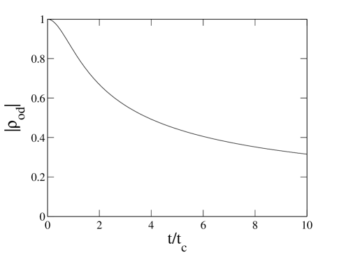
Figure 7: The decay of $|\rho_{\rm od}^{(\rm red)}|$ as a function of $t/t_{c}$.

To apply the above result to an atomic condensate, we consider the relevant temperature scale at $T\sim 100nK$ and assume that a particular observable excitation has $\delta\sim 10^{-1}$. In this case, we see that $t_{c}\sim 10^{-3}$ seconds, less than the life times of many observed ground states. We can also try to obtain an approximation to the coherence time of the condensate ground state. Taking the atom number as $N\sim 10^{6}$, if the ground state is assumed a coherent state, than the number fluctuations is of the order of $\Delta N=\sqrt{N}$. The inertia parameter $I$ is proportional to $I\sim N^{2/5}$ you96 ; alpha in the Thomas-Fermi limit, which gives $\delta=\left[(N+\Delta N)^{2/5}-N^{2/5}\right]/N^{2/5}=2\Delta N/5N$, or $\delta\sim 10^{-3}$. Substituting this in, we find $t_{c}\sim 10^{-1}$ seconds, much larger than for the excited state, as to be expected. Furthermore, the result for the ground state life time is in agreement with our previous calculation in sect. II.

IV quasi-particles in a condensate

IV.1 A thermal state

We now focus on the Hamiltonian of a dilute, weakly interacting atomic Bose gas huang

$$\mathcal{H}=\sum_{k}E_{k}a_{k}^{\dagger}a_{k}+\frac{\tilde{u}}{2}\sum_{k,p,q}a_{p+q}^{\dagger}a_{k-q}^{\dagger}a_{k}a_{p}.$$ (28)

Omitting the $3^{rd}$ and $4^{th}$ order operator terms in the non-condensed mode (${k\neq 0}$), we can partition the Hamiltonian into

$$\mathcal{H} = \mathcal{H}_{z}+\mathcal{H}_{e},$$ (29)

$$\mathcal{H}_{z} = \frac{\tilde{u}}{2}(\hat{n}_{0}^{2}-\hat{n}_{0}),$$

$$\mathcal{H}_{e} = \sum_{k\neq 0}\left[\left(E_{k}+2\tilde{u}\hat{n}_{0}\right)\hat{n}_{k}+\frac{\tilde{u}}{2}\left(a_{k}^{\dagger}a_{-k}^{\dagger}a_{0}a_{0}+h.c.\right)\right],$$

where $\hat{n}_{k}=a_{k}^{\dagger}a_{k}$ is the mode occupation. The above two parts of the Hamiltonian actually do not commute with each other, as we can easily check that

$$[\mathcal{H}_{z},\mathcal{H}_{e}]=\frac{\tilde{u}^{2}}{2}\sum_{k\neq 0}\left[a_{k}^{\dagger}a_{-k}^{\dagger}\left(-\hat{n}_{0}a_{0}^{2}-a_{0}^{2}\hat{n}_{0}+a_{0}^{2}\right)-h.c.\right].\hskip 12.0pt$$ (30)

Neglecting the quantum nature of $a_{0}$ in $\mathcal{H}_{e}$, we can replace $\hat{n_{0}}/V$ by $\rho_{0}=N_{0}/V$, and get

$$\mathcal{H}_{e}=\sum_{k\neq 0}\left[\epsilon_{k}\hat{n}_{k}+\frac{u_{0}\rho_{0}}{2}(a_{k}^{\dagger}a_{-k}^{\dagger}+h.c.)\right],$$ (31)

where we have defined $\epsilon_{k}=E_{k}+2u_{0}\rho_{0}-\mu_{0}$ with $\mu_{0}=u_{0}\rho_{0}$ for a coherent condensate state. In this approximation, $[\mathcal{H}_{z},\mathcal{H}_{e}]=0$ at the cost of sacrificing the conservation of $N_{\rm total}=\sum_{k}n_{k}$.

The quadratic Hamiltonian (31) can be diagonalized with the Bogoliubov quasi-particles into the canonical form

$$\mathcal{H}_{e}=\sum_{k\neq 0}\omega_{k}b_{k}^{\dagger}b_{k}+const.,$$ (32)

with $\omega_{k}=[\epsilon_{k}^{2}-u_{0}^{2}\rho_{0}^{2}]^{1/2}$ greiner and $b_{k}=Sa_{k}S^{-1}$. $S$ is the multi-mode squeeze operator haque06 .

In order to conserve the particle number density in the condensate, we include a chemical potential term in the zero mode Hamiltonian

$$\mathcal{H}_{z}=\frac{\tilde{u}}{2}(\hat{n}_{0}^{2}-\hat{n}_{0})-\mu_{0}\hat{n}_{0}.$$ (33)

The ground state of such a system will be a Fock number state $|N_{0}\rangle$ with $N_{0}=\mu_{0}V/u_{0}+1/2$. We assume that although $N_{0}$ and $V$ may fluctuate, their ratio $\rho_{0}$ is always a constant, as in the thermodynamic limit. In this case, $\mathcal{H}_{z}$ becomes

$$\mathcal{H}_{z}=\frac{u_{0}\rho_{0}}{2N_{0}}(\hat{n}_{0}^{2}-\hat{n}_{0})-\mu_{0}\hat{n}_{0}.$$ (34)

Substituting $\mu_{0}=u_{0}\rho_{0}-u_{0}\rho_{0}/2N_{0}$, we get

$$\mathcal{H}=\frac{u_{0}\rho_{0}}{2N_{0}}\hat{n}_{0}^{2}-\rho_{0}u_{0}\hat{n}_{0}+\mathcal{H}_{e}.$$ (35)

For a coherent condensate state with $\mu_{0}=u_{0}\rho_{0}$, we could immediately get this result by neglecting the second term in Eq. (34), consistent with the non-zero momentum part of the Hamiltonian.

The ground state, which we denote as $|\Phi\rangle$, has $N_{0}$ bosons in the zero momentum state and no quasi-particle excitations at all, i.e., for $k\neq 0$,

$$b_{k}|\Phi\rangle = 0$$ (36)

$$= Sa_{k}S^{-1}|\Phi\rangle,$$

or

$$a_{k}S^{-1}|\Phi\rangle=0,$$ (37)

and

$$|\Phi\rangle=S|{\rm vac}\rangle.$$ (38)

Therefore, the quasi-particle vacuum state $|\Phi\rangle$ is in fact a squeezed vacuum of atoms with nonzero $k$.

Now, we consider a setup with $n$ atoms in the condensate mode and $m$ quasi-particle excitations at a certain, single $k$ mode, while all other modes are empty. We will denote such a state by $|n,m\rangle$

$$\hat{n}_{0}|n,m\rangle = n|n,m\rangle,$$ (39)

$$\hat{n}_{k^{\prime}}|n,m\rangle = m\,\delta_{k,k^{\prime}}|n,m\rangle.$$ (40)

In the single-particle excitation regime $E_{k}\gg\rho_{0}u_{0}$, each quasi-particle excitation reduces the number of condensate atoms by one. In this case, the energy of this state can be written as

$$\mathcal{H}|n,m\rangle = E_{m}^{(n)}|n,m\rangle$$ (41)

$$= \left[\frac{u_{0}\rho_{0}n^{2}}{2(N_{0}-m)}-u_{0}\rho_{0}n+m\omega\right]|n,m\rangle,\hskip 12.0pt$$

where we simply denote $\omega=\omega_{k}$.

Assume the system can be initially prepared with no quasi-particle excitation at all, but is in a Boltzmann weighted distribution over the states $|n,0\rangle$, i.e.,

$$\rho(t=0)\propto\sum_{n}{\rm e}^{-\beta E_{0}^{(n)}}|n,0\rangle\langle n,0|.$$ (42)

This state will allow us to study the number fluctuations due to unknown nonzero temperature constituents that make up the occupations of the thin spectrum wezel06 . The summation index can take any positive integers and therefore the summation should be over $0\leq n<+\infty$. However, we note that the maximum of $E_{0}^{(n)}$ is at $N_{0}\gg 1$, and because it becomes extremely small for small values of $n$, we can extend the summation to be over the full range $-\infty<n<+\infty$ and replace it with an integral in the continuous limit as done in the following.

Excitation of a quasi-particle brings each $|n,0\rangle$ to $|n,1\rangle$. The off diagonal element of the resulting state will evolve according to

$$\rho_{\rm od}(t>0) \propto \int_{-\infty}^{\infty}{\rm e}^{-\beta E_{0}^{(n)}}{\rm e}^{-\frac{i}{\hbar}(E_{1}^{(n)}-E_{0}^{(n)})t}dn$$ (43)

$$\propto \int_{-\infty}^{\infty}{\rm e}^{(-\beta u_{0}\rho_{0}/2N_{0}+itu_{0}\rho_{0}/2\hbar N_{0}^{2})n^{2}+\beta\rho_{0}u_{0}n}dn$$

$$\propto \sqrt{\pi}\frac{\exp\left(\frac{\beta^{2}\rho_{0}^{2}u_{0}^{2}}{2\beta u_{0}\rho_{0}/N_{0}-2itu_{0}\rho_{0}/\hbar N_{0}^{2}}\right)}{\sqrt{\beta u_{0}\rho_{0}/2N_{0}-itu_{0}\rho_{0}/2\hbar N_{0}^{2}}},$$

which gives

$$|\rho_{\rm od}(t)|^{2}\propto\frac{\exp\left(\frac{\beta^{3}N_{0}^{3}u_{0}\rho_{0}}{\beta^{2}N_{0}^{2}+t^{2}/\hbar^{2}}\right)}{\sqrt{\beta^{2}+t^{2}/\hbar^{2}N_{0}^{2}}},$$ (44)

after omitting terms with only a phase factor. Although the denominator and the numerator have quite different forms, we find that both decay in a time proportional to $t_{c}\sim\hbar N_{0}/k_{B}T$. This is the same result that Wezel et. al. have found for a crystal wezel06 . The decay of this function is plotted in Fig. 8 for unit values of parameters.

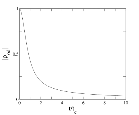
Figure 8: The relative decay of the off diagonal element in equation (44) as a function of $t/t_{c}$ for unit values of parameters.

For an atomic Bose-Einstein condensate, the relevant parameters are $N_{0}\sim 10^{6}-10^{8}$ and $T\sim 10^{-8}-10^{-7}$ K. These then lead to $t_{c}\sim 10^{2}-10^{5}$ seconds, which is a time much larger than both the theoretical and observed ground state life times. However, this is the life time for a single quasi-particle excitation, i.e., for $m=1$. It is easy to show that the collapse time is inversely proportional to $m$ for m values not too large. An easily tractable excitation should have $m\sim N_{0}$ and this gives $t_{c}\sim 10^{-4}-10^{-3}$ seconds, much smaller than both the observed and expected ground state life times.

The study of temperature dependence for the damping rates of Bogoliubov excitations of any energy has been carried out before using perturbation theory. A linear temperature dependence was found gora , surprisingly coinciding with the linear dependence found here based on the decoherence of the thin spectrum. Our result clearly would make a quantitative contribution to the total decay of the quasiparticles, although we note that our calculation is limited only to the single-particle excitation regime as we have used $\epsilon_{k}=E_{k}\gg u_{0}\rho_{0}$. In the phonon branch corresponding to the low-lying collective excitations out of a condensate, more complicated temperature dependencies may occur liu . In contrast to damping mechanisms based upon excitation collision processes in the condensate, the thin spectrum caused decay rate shows no system specific dependencies, apart from the dependencies on temperature and the number of atoms. It is independent of the interatomic interaction strength or the scattering length, and the quasiparticle spectrum. This is due to the fact that thin spectrum emerges as a result of a global symmetry breaking in a quantum system so that local properties of the system do not contribute to the associated decay rate.

IV.2 A thermal coherent state

We now generalize the above idea to a thermal coherent occupation of the zero-mode. The initial density matrix becomes in this case

$$\rho_{\rm od}(0) = Z^{-1}\sum_{n}{\rm e}^{-\beta E_{0}^{(n)}}D(\alpha)|n,0\rangle\langle n,0|D^{\dagger}(\alpha)$$ (45)

$$= Z^{-1}\sum_{nmm^{\prime}}{\rm e}^{-\beta E_{0}^{(n)}}C_{m}(n,\alpha)C_{m^{\prime}}^{*}(n,\alpha)$$

$$|m,0\rangle\langle m^{\prime},0|.$$

The system is now brought into a superposition of no quasi-particle and one quasi-particle state, i.e., $|n,0\rangle\rightarrow(|n,0\rangle+|n,1\rangle)/\sqrt{2}$. After further time evolution, the state becomes

$$\rho(t) = Z^{-1}\sum_{nmm^{\prime}}\sum_{kk^{\prime}=0,1}\frac{{\rm e}^{-\beta E_{0}^{(n)}}}{2}C_{m}(n,\alpha)C_{m^{\prime}}^{*}(n,\alpha)$$ (46)

$${\rm e}^{-\frac{i}{\hbar}(E_{1}^{(m)}-E_{0}^{(m^{\prime})})t}|m,k\rangle\langle m^{\prime},k^{\prime}|,$$

giving rise to the reduced density matrix and its off diagonal element below

$$\rho^{\rm(red)} = Z^{-1}\sum_{nl}\sum_{kk^{\prime}=0,1}\frac{{\rm e}^{-\beta E_{0}^{(n)}}}{2}|C_{l}(n,\alpha)|^{2}$$ (47)

$${\rm e}^{-\frac{i}{\hbar}(E_{k}^{(l)}-E_{k^{\prime}}^{(l)})t}|k\rangle\langle k^{\prime}|,$$

$$\rho^{\rm(red)}_{\rm od} = Z^{-1}\sum_{nl}\frac{{\rm e}^{-\beta E_{0}^{(n)}}|C_{l}(n,\alpha)|^{2}}{2}{\rm e}^{-\frac{i}{\hbar}(E_{1}^{(l)}-E_{0}^{(l)})t}.\hskip 24.0pt$$ (48)

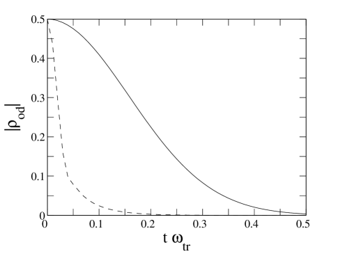
Figure 9: Decay of the off diagonal element at $T=10$ nK as a function of $t\omega_{tr}$. Dashed line shows the decay in the case of the thermal coherent occupation and the solid line shows that in the case of the thermal occupation.

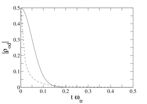
Figure 10: Decay of the off diagonal element for $T=100$ nK and thermal coherent occupation of the zero mode as a function of $t\omega_{tr}$. Dashed line shows the decay in the case of the thermal coherent occupation and the solid line shows that in the case of the thermal occupation.

Figs. 9 and 10 show the early time decay at temperatures of $10$ nK and $100$ nK respectively. It is seen that the decay time for a thermal occupation, which we have studied in the preceding subsection, exhibits stronger temperature sensitivity, whereas the decay time for the thermal coherent occupation is not changed very much by temperature. Therefore, we conclude that for a thermal coherent occupation, the main reason for the decay of the off diagonal element is the decay of the zero mode distribution. However, if there is solely thermal occupation, no decay of the zero mode occurs, and the off diagonal element decays only because of the temperature. In the previous section, we have seen that the decay rate due to the thin spectrum and the decay rate due to the excitation collision processes show the same temperature dependence qualitatively. In the case of coherent thermal occupation of the zero mode, qualitative differences appear in the temperature dependence of the decay time due to the different decay mechanisms. Any remaining coherence in the zero-mode at non-zero temperatures makes the condensate decay less sensitive to temperature.

V More than one broken symmetry

A system may have more than one spontaneously broken symmetry. For example, in addition to a broken gauge symmetry, the formation of vortices breaks the rotational symmetry of a condensate in a spherically symmetric trap vortex . Furthermore, rotational symmetry can also be broken ozgur for a multi-component or a spinor condensate mc_bec . When more than one continuous symmetry is broken, there will exist as many gapless modes as for the broken symmetries, each with its own thin spectrum. In this section, we briefly consider the effect of more than one thin spectrum.

Consider a general effective Hamiltonian with two gapless modes

$$\mathcal{H}=\alpha_{1}p_{1}^{2}+\alpha_{2}p_{2}^{2}+\alpha_{12}p_{1}p_{2}+\sum_{k}\hbar\omega_{k}b^{\dagger}_{k}b_{k},$$ (49)

which after a canonical transformation, reduces to

$$\mathcal{H}=\alpha_{1}^{\prime}{p_{1}^{\prime}}^{2}+\alpha_{2}^{\prime}{p_{2}^{\prime}}^{2}+\sum_{k}\hbar\omega_{k}b^{\dagger}_{k}b_{k}.$$ (50)

Without loss of generality, we use this form of the Hamiltonian and henceforth omit the primes. The observable state will be denoted by $n$, and an easy extension leads to $\mathcal{H}|n,p_{1},p_{2}\rangle=E^{(p_{1},p_{2})}_{n}|n,p_{1},p_{2}\rangle$ with $E^{(p_{1},p_{2})}_{n}=E^{(0,0)}_{n}+\alpha_{1}p_{1}^{2}+\alpha_{2}p_{2}^{2}$. More generally, the primary excitation may affect both inertia terms in the two thin spectra, which may themselves be coupled, i.e., $\alpha_{1}=\alpha_{1}(n,p_{2})$ and $\alpha_{2}=\alpha_{2}(n,p_{1})$. Expanding around the small $p_{1}$ and $p_{2}$ , we find around $p_{j}=0$

$$E^{(p_{1}p_{2})}_{n} = E^{(0,0)}_{n}+\left[\alpha_{1}(n,0)+\alpha^{\prime}_{1}(n,0)p_{2}+...\right]p_{1}^{2}+$$ (51)

$$\left[\alpha_{2}(n,0)+\alpha^{\prime}_{2}(n,0)p_{1}+...\right]p_{2}^{2}$$

$$\simeq E^{(0,0)}_{n}+\alpha_{1}(n,0)p_{1}^{2}+\alpha_{2}(n,0)p_{2}^{2},$$

up to the second orders in $p_{j}$. Thus, we can safely ignore the inertia terms’ dependence on other’s thin excitations to the first approximation and let $\alpha_{1}(n,p_{2})=\alpha_{1}(n)$. Instead of (23) we now find

$$\rho^{\rm(red)}_{\rm od}=Z^{-1}\left[\sum_{p_{1}p_{2}}{\rm e}^{-\beta E_{0}^{(p_{1},p_{2})}}{\rm e}^{-\frac{i}{\hbar}(E_{1}^{(p_{1},p_{2})}-E_{0}^{(p_{1},p_{2})})t}\right]C_{1}C_{0}^{*}.\hskip 12.0pt$$ (52)

Upon substituting the approximate forms for the $E_{j}$s, we find

$$\begin{split}\rho^{\rm(red)}_{\rm od}=&Z^{-1}{\rm e}^{-\beta E_{0}^{(0,0)}}{\rm e}^{-\frac{i}{\hbar}(E_{1}^{(0,0)}-E_{0}^{(0,0)})t}\\ &\sum_{p_{1},p_{2}}{\rm e}^{-\frac{i}{\hbar}\left[\alpha_{1}(1)-\alpha_{1}(0)\right]p_{1}^{2}t}{\rm e}^{-\frac{i}{\hbar}\left[\alpha_{2}(1)-\alpha_{2}(0)\right]p_{2}^{2}t}\\ &{\rm e}^{-\beta[\alpha_{1}(0)p_{1}^{2}+\alpha_{2}(0)p_{2}^{2}]}C_{1}C_{0}^{*},\end{split}$$ (53)

$$\rho^{\rm(red)}_{\rm od}=({\rm const.}){\rm e}^{-t/t^{(1)}_{c}}{\rm e}^{-t/t^{(2)}_{c}}.$$ (54)

Thus, we see that the collapse due to different thin spectra do not influence each other severely. They combine to give a resulting decay with a simple single decay time

$$t_{c}=\left(\frac{1}{t^{(1)}_{c}}+\frac{1}{t^{(2)}_{c}}\right)^{-1}.$$ (55)

VI Conclusion

Based on a toy model calculation for the decoherence dynamics of a coherent ground state condensate, we have generalized the calculations of the dephasing times to cases of a squeezed coherent ground state as well as a thermal coherent ground state. The numerical results for a squeezed ground state reveal that phase fluctuations increase its coherence lifetime mara ; ibloch , whereas temperature increases always decrease the lifetimes for ground state quantum coherence.

The dynamics of thin spectrum are shown to lead to decoherence, not just on the ground state, but on quasi-particle excitations, or superpositions of excitations. We have introduced simple approximations that allowed for the calculations of the decoherence lifetime of the condensate ground state as well as its coherence excitations. These calculations make possible the discussion of temperature effects in terms of the thermal and thermal coherent occupations of the zero mode. We find that the lifetimes for these two cases are of the same order of magnitude, although the lifetime for the latter shows a weak sensitivity on temperature, whereas that of the former displays a stronger sensitivity.

- (1) P. Kapitsa, Nature 141, 74 (1938); J. F. Allen and A. D. Misener, Nature 141, 75 (1938).
- (2) S. N. Bose, Z. Phys. 26, 178 (1924); A. Einstein, Sitzungsber. K. Preuss. Akad. Wiss. 22, 261 (1924); ibid 23, 3 (1925).
- (3) M. H. Anderson, J. R. Ensher , M. R. Matthews, C. E. Wieman, and E. A. Cornell, Science 269, 198 (1995); C. C. Bradley, C. A. Sackett, J. J. Tollett, and R. G. Hulet, Phys. Rev. Lett. 75, 1687 (1995); K. B. Davis, M. -O. Mewes, M. R. Andrews, N. J. van Druten, D. S. Durfee, D. M. Kurn, and W. Ketterle, Phys. Rev. Lett., 75, 3969 (1995).
- (4) E.M. Wright, D.F. Walls, and J.C. Garrison, Phys. Rev. Lett. 77, 2158 (1996).
- (5) M. Lewenstein and L. You, Phys. Rev. Lett. 77, 3489 (1996).
- (6) M. Greiner, O. Mandel, T. W. Hansch, and I. Bloch, Nature 419, 51 (2002).
- (7) J. van Wezel, J. Zaanen, and J. van den Brink, Phys. Rev. B 74, 094430 (2006).
- (8) J. van Wezel, J. van den Brink, and J. Zaanen, Phys. Rev. Lett. 94 230401 (2005).
- (9) J. van Wezel, J. van den Brink, arxiv:cond-mat/07043703 (2007).
- (10) P. Villain et. al, J. of Mod. Optics 44, 1775 (1997).
- (11) A. Imamoglu, M. Lewenstein, and L. You, Phys. Rev. Lett. 78, 2511 (1997).
- (12) L. Mandel and E. Wolf, Optical Coherence and Quantum Optics, Cambridge University Press (1995), page 1038.
- (13) G.-B. Jo, Y. Shin, S. Will, T. A. Pasquini, M. Saba, W. Ketterle, D. E. Pritchard, M. Vengalattore, and M. Prentiss, Phy. Rev. Lett. 98, 030407 (2007).
- (14) F. Gerbier, S. Folling, A. Widera, O. Mandel, and I. Bloch, Phys. Rev. Lett. 96, 090401 (2006).
- (15) A. Wünsche in Theory of Nonclassical States of Light, edited by V. V. Dodonov and V. I. Man’ko, (Taylor and Francis, New York, 2003).
- (16) S. M. Roy and V. Singh, Phys. Rev. D 25, 3413 (1982).
- (17) J. Goldstone, Nuovo Cim. 19, 154 (1961); Y. Nambu and G. Jona-Lasinio, Phys. Rev. 122, 345 (1961).
- (18) Z. F. Ezawa, Quantum Hall Effects, (World Scientific, New York, 2000), Chapter 4.
- (19) D. Forster, Hydrodynamic Fluctuations, Broken Symmetry, and Correlation Functions, (W.A. Benjamin Inc., New York, 1975), pg. 166.
- (20) M. Okumura and Y. Yamanaka, Prog. The. Phys. 111, 199 (2004).
- (21) K. Huang, Statistical Mechanics, (Wiley, New York, 1987).
- (22) W. Greiner, Quantum Mechanics—Special Chapters, (Springer-Verlag, New York, 1998), Chapter 6.
- (23) M. Haque and A. E. Ruckenstein, Phys. Rev. A 74, 043622 (2006); P. Navez, Mod. Phys. Lett. B 12, 705 (1998).
- (24) P. O. Fedichev and G. V. Shlyapnikov, Phys. Rev. A 58, 3146 (1998).
- (25) W. V. Liu, Phys. Rev. Lett. 79, 4056 (1997).
- (26) For a review of vortices in atomic condensates, please see: A. Fetter and A. Svidzinsky, J. Phys. Condens. Matter 13, R135 (2001).
- (27) S. Yi, O. E. Mustecaplioglu, and L. You, Phys. Rev. Lett. 90, 140404 (2003); Phys. Rev. A 68, 013613 (2003).
- (28) A. F. R. de Toledo Piza, Braz. Jour. of Phys. 34, 1102 (2004).