A New 3D Potential-Density Basis Set

Abstract

A set of bi-orthogonal potential-density basis functions is introduced to model the density and its associated gravitational field of three dimensional stellar systems. Radial components of our basis functions are weighted integral forms of spherical Bessel functions. We discuss on the properties of our basis functions and demonstrate their shapes for the latitudinal Fourier number $l=2$.

1 Introduction

Potential–density basis sets are used for expanding the solution of Poisson’s equation during N-body simulations and stability analysis of stellar systems. Spherical harmonics are the most efficient functions for expansions in the azimuthal and latitudinal directions but finding bi-orthogonal components in the radial direction, which are expressible in terms of ordinary or special functions, is not a straightforward task. A numerical method has been introduced by Weinberg (1999) for constructing the basis functions in the radial direction. His method always gives a bi-orthogonal set whose components oscillate in the radial direction. However, the amplitude of oscillations and the locations of zeros of such functions do not necessarily assure a good performance. Especially, when one of the peaks of radial components is higher than others [this happens for the Clutton-Brock (1973) and Hernquist & Ostriker (1992) functions], computations are rapidly biased. Here we use Clutton-Brock’s (1972) idea and construct a basis set using the weighted integral form of spherical Bessel functions. The functions that we find have shown a good performance in the stability analysis of spherical systems (Jalali & Hunter 2007).

2 A new potential–density pair

The Laplace operator is Hermitian, and therefore, its eigenfunctions always form a complete and bi-orthogonal set ([Arfken 1995, Arfken 1985]). A three dimensional generalization of Clutton-Brock’s (1972) method suggests to introduce

$$\Phi_{lmn}(r,\theta,\phi) = -Y_{lm}(\theta,\phi)\Phi_{ln}(r)=-Y_{lm}(\theta,\phi)\int_{0}^{\infty}j_{l}(kr/a)g_{ln}(k)dk,$$ (1)

$$\rho_{lmn}(r,\theta,\phi) = \frac{Y_{lm}(\theta,\phi)}{4\pi Ga^{2}}\rho_{ln}(r)=\frac{Y_{lm}(\theta,\phi)}{4\pi Ga^{2}}\int_{0}^{\infty}j_{l}(kr/a)g_{ln}(k)k^{2}dk,$$ (2)

as the potential and density basis functions. Here $g_{nl}(k)$ are some orthogonal functions and $a$ is a length scale. $j_{l}(r)$ and $Y_{lm}(\theta,\phi)$ are the spherical Bessel functions and spherical harmonics, respectively. Their combination $j_{l}(r)Y_{lm}(\theta,\phi)$ satisfies Poisson’s equation. It is straightforward to show that $\nabla^{2}\Phi_{lmn}=4\pi G\rho_{lmn}$. Denoting $L^{2l}_{n}$ as Laugerre functions and considering their orthogonality, the choice of $g_{ln}(k)=k^{l}L^{2l}_{n}(2k)e^{-k}$ leads to the following bi-orthogonality relation between $\Phi_{lmn}$ and $\rho_{lmn}$:

$$\int_{-\pi}^{\pi}\int_{0}^{\pi}\int_{0}^{\infty}\rho_{lmn}\Phi^{*}_{lmn}r^{2}drd\theta d\phi=-\delta_{l,l^{\prime}}\delta_{m,m^{\prime}}\delta_{n,n^{\prime}}\frac{a(2l+n)!}{2^{2l+4}Gn!}.$$ (3)

The above potential and density functions oscillate in the $r$-direction and the amplitude of oscillations decays slowly. Peaks of these basis functions accumulate near the center by increasing $n$, and therefore, they are suitable for stability analyses that utilize matrix methods. The first potential function in the radial direction is $\Phi_{00}(r)=-r^{-1}\arctan{r}$ whose profile falls off similar to $r^{-1}$ as $r\rightarrow\infty$. Our basis functions can be computed both numerically and analytically. Since the spherical Bessel functions and their combinations with Laugerre functions decay rapidly, definite integrals in (2.1) and (2.2) converge very fast by adopting standard numerical schemes. For instance, we have computed and displayed in Figure 1 the radial potential and density basis functions for $l=2$ and several values of $n$.

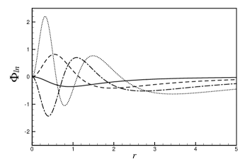
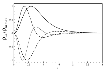
Figure 1: Potential (left) and density (right) basis functions for $l=2$. Solid, dashed, dash-dotted and dotted lines correspond to $n=$0, 1, 2, and 3, respectively. Densities have been scaled to their maximum values.

We have also examined the performance of our basis set in modeling the spherical and oblate Kuzmin-Kutuzov models. Our experiments show that taking a handful of expansion terms reconstructs the original model with a relative error less than %1.

3 Conclusions

Our basis functions constitute a bi-orthogonal set over the domain $0\leq r<\infty$. By adjusting the length scale $a$, it is possible to model stellar systems of different core radii and spatial extensions. The wave length of our radial basis functions decreases towards the center while their wave amplitudes are not changed substantially. These properties are useful for the instability analysis of three dimensional stellar systems, for instabilities occur in central regions of stellar systems and accurate calculation of perturbed physical quantities demands high-resolution functions near the center.

References

- [Arfken 1995] Arfken, G. 1985, Mathematical Methods for Physicists, 3rd ed., (Academic Press)
- [Clutton-Brock 1972] Clutton-Brock, M. 1972, Ap&SS 16, 101
- [Clutton-Brock 1973] Clutton-Brock, M. 1973, Ap&SS 23, 55
- [Jalali & Hunter 2007] Jalali, M.A., Hunter C. 2007, to be submitted
- [Hernquist & Ostriker 1992] Hernquist L., Ostriker J.P. 1992, ApJ 386, 375
- [Weinberg 1999] Weinberg M.D. 1999, AJ 117, 629