Statistics of Extreme Values in Time Series with Intermediate-Term Correlations

Abstract

It will be discussed the statistics of the extreme values in time series characterized by finite-term correlations with non-exponential decay. Precisely, it will be considered the results of numerical analyses concerning the return intervals of extreme values of the fluctuations of resistance and defect-fraction displayed by a resistor with granular structure in a nonequilibrium stationary state. The resistance and defect-fraction are calculated as a function of time by Monte Carlo simulations using a resistor network approach. It will be shown that when the auto-correlation function of the fluctuations displays a non-exponential and non-power-law decay, the distribution of the return intervals of extreme values is a stretched exponential, with exponent largely independent of the threshold. Recently, a stretched exponential distribution of the return intervals of extreme values has been identified in long-term correlated time series by Bunde et al. (2003) and Altmann and Kantz (2005). Thus, the present results show that the stretched exponential distribution of the return intervals is not an exclusive feature of long-term correlated time series.

I INTRODUCTION

The puzzling questions posed by the observations of climate changes christensen ; mudelsee ; tebaldi ; perry ; goswami ; ice_1 ; ice_3 have recently provided further motivations to the investigation of extreme events and dynamics gumbel ; storch ; kotz ; sornette ; racz ; salvadori . In particular, the statistics of the return times (RTs) of extreme values is one of the subjects that have recently attracted the attentions of many authors schmitt ; bunde_physa2003 ; bunde_prl2005 ; kantz_2005 ; upon05 ; pen_epj . Return times (or intervals) $r_{q}$, of the extreme values of a fluctuating quantity $x(t)$, associated with the overcoming of a given threshold $q$, can be defined storch ; bunde_physa2003 as the time intervals between two consecutive occurrences of the condition $x(t)>q$ . In the case of uncorrelated events it is easy to show that the RTs are exponentially distributed storch ; kotz ; bunde_physa2003 . Exponential distributions describe the statistics of return intervals of prices in financial markets, wind speed data or daily precipitations in a given place for the same time windows storch ; bunde_physa2003 ; kantz_2005 .

On the other hand, in recent years it has been realized that several other important examples of time series display long-term correlations bunde_physa2003 ; bunde_prl2005 ; kantz_2005 . This is the case of physiological data (heartbeats bunde_prl2000 ; ashkenazy and neuron spikes davidsen ), hydro-meteorological records (daily temperatures bunde_physa2003 ; kantz_2005 ; koscielny_prl98 ; salvadori ), geophysical or astrophysical data (occurrence of earthquakes bak ; corral or solar flares boffetta ), internet traffic bunde_physa2003 and stock market volatility kantz_2005 ; liu records. Long-term correlated time series are characterized by an auto-correlation function, $C_{x}(s)$, decaying as a power-law:

$$C_{x}(s)=<x_{i}x_{i+s}>={1\over N-s}\sum_{i=1}^{N-s}x_{i}x_{i+s}\sim s^{-\gamma_{x}}$$ (1)

where the correlation exponent $\gamma_{x}$ ranges between 0 and 1 (normalized series $\{x_{i}\}_{i=1,...N}$ with zero average and unit variance are considered). Therefore, in these conditions, the mean correlation time $\tau$ diverges ($\tau$ is defined as the integral over $s$ of $C_{x}$). The effect of long-terms correlations on the RT statistics has been recently studied by Bunde et al. bunde_physa2003 ; bunde_prl2005 and by Altmann and Kantz kantz_2005 . Both these studies were performed on the ground of numerical calculations on Gaussian and long-term correlated time series generated by the Fourier transform technique and by imposing a power-law decay of the power spectrum makse . The main conclusions of Bunde at al. were the following. i) The mean return interval $R_{q}$ is unchanged by the presence of long-terms correlations. ii) The distribution of the RTs becomes stretched exponential:

$$P_{q}(r)=a/R_{q}\ \exp\bigl{[}-\bigl{(}b\ \ r/R_{q}\bigr{)}^{\gamma}\bigr{]}$$ (2)

where the exponents $\gamma$ and $\gamma_{x}$ were found to be equal. iii) The RTs themselves are long-term correlated with a correlation exponent $\gamma^{\prime}\approx\gamma_{x}$. Actually, as noted by Altmann and Kantz kantz_2005 , the statement i) is true in general and can be identified with Kac’s lemma kac introduced in the context of dynamical systems while the statement iii) is true only in very special conditions kantz_2005 . Moreover, it must be noted that the results ii) and iii) only apply to linear time series (i.e. to series whose properties are completely defined by the power spectrum and by the probability density) kantz_2005 ; bunde_prl2005 . However, apart from this restriction, the stretched exponential distribution of the RTs can be considered a general feature in presence of long-term correlations in a time series kantz_2005 ; bunde_prl2005 . This feature has important consequences on the observation of extreme events: indeed it implies a strong enhancement of the probability of having return intervals well below and well above $R_{q}$, in comparison with the occurrence of extreme events in an uncorrelated time series. Furthermore, it must be noted kantz_2005 that the distribution in Eq. (2) only depends on the parameter $\gamma$, being $a$ and $b$ function of $\gamma$.

Here it will be considered the effect on the distribution of the RTs of the presence of finite-term correlations with non-exponential decay, a situation which can occur in systems which are approaching criticality, where intermediate behaviors with non-exponential and non-power-law decay of correlations can emerge sornette . Thus, in the next section it will be analyzed the RT statistics of extreme values of the resistance ad defect-fraction fluctuations displayed by a resistor with granular structure in a nonequilibrium stationary state pen_msn .

II METHOD AND RESULTS

The time series analyzed consist in the fluctuations of resistance and defect-fraction of a thin resistor with granular structure, biased by an external current $I$ and in contact with a thermal bath at temperature $T$. The resistance values are calculated by using the multi-species resistor network (MSN) model pen_msn . The MSN model describes a conducting film with granular structure as a resistor network made by different species of elementary resistors. Precisely, the resistor species are distinguished by their resistances and by their energies associated with thermally activated stochastic processes of breaking and recovery of the elementary resistors. The broken elementary resistors, named defects, correspond to resistors of resistance about $10^{9}$ higher than that of normal resistors. As a result of the competition between pairs of breaking and recovery processes for each species, the network can reach a stationary state whose properties will be dependent on the external conditions. The resistance and the defect fraction of the network are calculated by Monte Carlo simulations as a function of the time for different temperatures pen_msn . All the details about the MSN model and its results can be found in Ref. pen_msn, . It should be noted, however, that this model provides a correlation time of the resistance fluctuations dependent on the temperature: $\tau\sim(T-T^{*})^{-\theta}$ with ${\theta}=2.7$, thus diverging for $T\rightarrow T^{*}$. As a result, the power spectral density of the resistance fluctuations shows a $1/f^{\alpha}$ dependence of frequency, with ${\alpha}\approx 1$ for $T\leq T^{*}$. It should be also noted that the MSN model represents an extension to systems characterized by $1/f$ noise of a previous model existing in the literature, the stationary and biased resistor network (SBRN) model pen_pre ; pen_physa ; pen_prb . In any case, it must be underlined that, apart from the specific system described by the MSN model, the method used here for generating the time series can be also viewed as a pure numerical algorithm for generating numerical series with different and tunable correlation properties.

Figure 1: Normalized $x(t)$ signal (zero average and unit variance). Here the original records consist of resistance fluctuations calculated at $400$ K. The time is expressed in simulation steps.

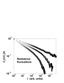
Figure 2: Auto-correlation functions of the resistance fluctuations calculated at $300$ K (up triangles), $400$ K (down triangles) and $500$ K (diamonds). The grey solid curves represent the best-fit with the function given in Eq. (3), while the grey dashed curve shows the best-fit with a power-law.

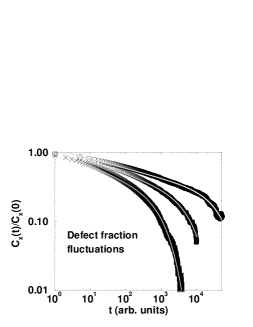
Figure 3: Auto-correlation functions of the defect-fraction fluctuations calculated at $300$ K (up circles), $400$ K (squares) and $500$ K (crosses). The grey solid curves represent the best-fit with the function given in Eq. (3).

Long $R(t)$ and $p(t)$ time series (typically made of $1\div 2\times 10^{6}$ records) have been generated and analyzed for different temperatures. Here $R$ indicates the resistance of the network expressed in Ohm and $p$ the defect-fraction, while the time $t$ is expressed in iteration steps. The analysis has been performed by considering normalized series: $x(t)\equiv(R(t)-<R>)/\sigma$, where $<R>$ is the average value of the network resistance and $\sigma$ the root-mean-square deviation from the average (a similar procedure has been adopted for the $p(t)$ series). The following quantities have been considered: the auto-correlation function, the PDF of the $x$ records, the return intervals $r_{q}$ of the extreme values for different threshold $q$ and their distribution $P_{q}(r)$ ($q$ is expressed in units of $\sigma$). All the results shown here are obtained by considering a network of size $75\times 75$, biased by a current $I=1.0$A and made by 15 species of resistors. The details concerning the network can be found in Ref. pen_msn, .

Figure 1 displays a typical trend of $x(t)$. Only a small portion of the total number of records, $N=2\times 10^{6}$, is shown. In this case $x(t)$ represents the normalized resistance fluctuations calculated at a temperature of $400$ K. The probability density of several $x(t)$ series has been also analyzed. It has been found that the PDF of the resistance fluctuations presents a significant non-Gaussianity that progressively increases at higher temperatures (going from $300$ to $500$ K) pen_msn ; pen_physa ; bramwell_nat , while the PDF of the defect-fraction fluctuations is Gaussian at all the temperatures.

Figure 2 reports the auto-correlation functions, $C_{x}(t)$, of three resistance fluctuation time series obtained for three different temperatures. Precisely, the three black curves correspond to a temperature of $300$, $400$ and $500$ K respectively going from the upper to the lower one. The grey dashed curve shows the best-fit to the $C_{x}$ data at $300$ K with a power-law of exponent $\gamma=0.22$, while the grey solid curves represent the best-fit to the data at $400$ and $500$ K with the function:

$$C_{x}(s)=C_{0}t^{-h}\exp(-t/u)$$ (3)

The fitting parameters are $C_{0}=1.23$, $h=0.30$ and $u=1.42\times 10^{4}$ for the data at $400$ K and $C_{0}^{\prime}=0.98$, $h^{\prime}=0.36$ and $u^{\prime}=1.51\times 10^{3}$ for the data at $500$ K. Many other functions have been also considered for the best-fit of the $C_{x}$ data. However, it has been found that the function in Eq. (3) optimizes the best-fit procedure with the minimum numbers of fitting parameters. By using Eq. (3), it is possible to calculate the correlation times characterizing the resistance fluctuations: $\tau=1051$ at $400$ K and $\tau=148$ at $500$ K (see Ref. pen_msn, for further details). Figure 3 shows the auto-correlation functions of the defect-fraction times series obtained at $300$, $400$ and $500$ K (black curves, again going from the upper to the lower one) and the best-fit to the $C_{x}$ data with Eq. (3) (grey solide curves). The fitting parameters are $C_{0}=1.12$, $h=0.14$ and $u=5.96\times 10^{4}$ for the data at $300$ K, $C_{0}^{\prime}=1.19$, $h^{\prime}=0.19$ and $u^{\prime}=8.17\times 10^{3}$ for the data at $400$ K and $C_{0}^{\prime\prime}=1.08$, $h^{\prime\prime}=0.23$ and $u^{\prime\prime}=1.29\times 10^{3}$ for the data at $500$ K. The correlation times are: $\tau=1.40\times 10^{4}$ at $300$ K, $\tau=1653$ at $400$ K and $\tau=306$ at $500$ K.

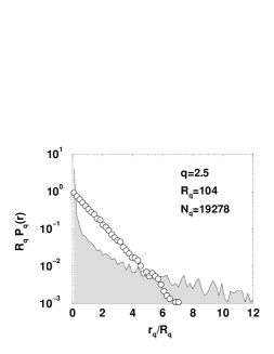
Figure 4: Distribution of the return intervals for values above the threshold $q=2.5$ (dashed black curve at the border of the grey area) obtained from the resistance fluctuations calculated at $300$ K (long-term correlated records). For comparison, the distribution of the return intervals for the same threshold value and obtained after shuffling the data is shown by circles.

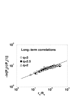
Figure 5: Double-logarithmic plot of the normalized probability density of the return intervals for different threshold values $q$. The $x(t)$ records are the same of Fig. 4, i.e. they present long-term correlations. The slope of the dashed line is 0.3.

Let us start the analysis of the return intervals by considering first the RT distribution for extreme values of the resistance fluctuations at $300$ K. As pointed out by Fig. 2, in this case $C_{x}$ scales as a power-law over more than four orders of magnitude, indicating the existence of long-term correlations. Figure 4 reports the distribution of $r_{q}$ for $q=2.5$ in semi-logarithmic plot. Precisely, a normalized representation has been adopted for convenience, by reporting the product of mean return interval $R_{q}$ for the probability density $P_{q}(r)$ as a function of the ratio $r_{q}/R_{q}$. For comparison, the distribution of $r_{q}$ for the same threshold, obtained after shuffling the $x(t)$ records is also shown. Thus Fig. 4 highlights the typical effect of long-term correlations: strong enhancement of the probability of having return intervals well below and well above $R_{q}$, in comparison with the occurrence of extreme values in uncorrelated time series, as described in Refs. bunde_physa2003, ; bunde_prl2005, ; kantz_2005, . Actually, the distribution of $r_{q}$ is found to be a stretched exponential, in agreements with the results of Refs. bunde_physa2003, ; bunde_prl2005, ; kantz_2005, . This is shown in Fig. 5, which reports a double-logarithmic plot of the normalized probability density of the $r_{q}$ as a function of the ratio $r_{q}/R_{q}$ and for different thresholds. In this representation, the slope of the dashed line directly provides the exponent $\gamma$ in Eq. (2). As expected bunde_physa2003 ; bunde_prl2005 ; kantz_2005 , $\gamma=0.3\approx\gamma_{x}$.

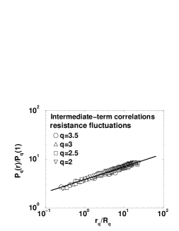
Figure 6: Double-logarithmic plot of the normalized probability density of the return intervals for different threshold values $q$. In this case the data (resistance fluctuations at $400$ K) are no more long-term correlated but exhibit intermediate-term correlations. The slope of the dashed line is 0.26.

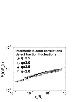
Figure 7: Double-logarithmic plot of the normalized probability density of the return intervals for different threshold values $q$. Also in this case the data (defect-fraction fluctuations at $400$ K) are characterized by intermediate-term correlations. The slope of the dashed line is 0.23.

Now, let us consider the RT distribution of extreme values for time series with finite correlation time and slow, non-exponential decay of correlations: a situation that can be called of ”intermediate-term correlations”. As shown by Figs. 2 and 3, the auto-correlation functions of the resistance fluctuations at $400$ and $500$ K (i.e. at $T>T^{*}$) and of the defect-fraction fluctuations at $300\div 500$ K are well described by Eq. (3). Thus, these series just exhibit this intermediate behavior of the time correlations. Figures 6 and 7 display double-logarithmic plots of the normalized probability density of the $r_{q}$ values calculated for the fluctuations at $400$ K respectively of the resistance and of the defect-fraction. Different thresholds $q$ ranging from $2$ to $3.5$ are considered in both cases. The slope of the solid line is 0.26 and 0.23, respectively for the case of Figs. 6 and 7. Figures 6 and 7 show that the distribution of the return intervals of extreme values of these series is well described by a stretched exponential and that the value of the exponent $\gamma$ is independent of the threshold $q$ in a large range of $q$-values. This occurs even in absence of long-term correlations and in presence of a finite correlation time.

III CONCLUSIONS

The distribution of return intervals of extreme values has been studied in several time series with different correlation properties: long-term and finite-term correlations. Precisely, it has been analyzed the return interval distribution of the fluctuations of resistance and defect-fraction displayed by a resistor with granular structure in nonequilibrium stationary states at different temperatures T. The resistance fluctuations were calculated by using the MSN model which is based on a resistor network approach pen_msn . It has been found that when the auto-correlation function displays a non-exponential and a non-power-law decay, the distribution of the return intervals is well described by a stretched exponential with exponent $\gamma$ largely independent of the threshold $q$. This result shows that the stretched exponential distribution describes the distribution of the return intervals of extreme values not only when long-term correlations are present in the time series kantz_2005 ; bunde_physa2003 ; bunde_prl2005 , but even when finite-term correlations with non-exponential decay exist among the records, a situation typical of many systems which are approaching criticality.

- (1) J. H. Christensen, O. B. Christensen, “Severe summertime flooding in Europe”, Nature, 421, pp. 805-806, 2003.
- (2) M. Mudelsee, M. Börhgen and G. Tetzlaff, “No upward trends in the occurrence of extreme floods in central Europe”, Nature, 425, pp. 166-168, 2003.
- (3) G. A. Meehl and C. Tebaldi, “More intense, more frequent and longer lasting heat weaves in the 21st century”, Science, 305, pp. 994-997, 2004.
- (4) A. L. Perry, P. J. Low, J. R. Ellis and J. D. Reynolds, “Climate change and distribution shift in marine fishes”, Science, 308, pp. 1912-1915, 2005.
- (5) B. N. Goswami, V. Venugopal, D. Sengupta, M. S. Madhusoodanan and P. K. Xavier, “Increasing trend of extreme rain events over India in a warming environment”, Science, 314, pp. 1442-1445, 2006.
- (6) J. T. Overpeck, B. L. Otto-Bliesner, G. H. Miller, D. R. Muhs, R. B. Alley and J. T. Kiehl,“Paleoclimatic evidence for future ice-sheet instability and rapid seal-level rise”, Science, 311, pp. 1747-1750, 2006.
- (7) G. Ekström, M. Nettles and V. C. Tsai, “Seasonality and increasing frequency of Greenland glacial earthquakes”, Science, 311, pp. 1756-1758, 2006.
- (8) E. J. Gumbel, Statistics of Extremes, Columbia University Press, New York, 1958.
- (9) H. von Storch and F. W. Zwiers, Statistical Analysis in Climate Research, Cambridge University Press, Cambridge, 2001.
- (10) S. Kotz and S. Nadarajah, Extreme Value Distributions, Theory and Applications, Imperial College Press, London, 2002.
- (11) D. Sornette, Critical Phenomena in Natural Sciences, Chaos, Fractals, Selforganization and Disorder: Concepts and Tools, Springer, Berlin, 2004.
- (12) T. Antal, M. Droz, G. Györgyi, Z. Rácz, “ noise and extreme value statistics”, Phys. Rev. Lett., 87, pp. 24061-1-4, 2001.
- (13) G. Salvadori and C. De Michele “Statistical characterization of temporal structure of storms”, Adv. Water Res., 29, pp. 827-842, 2006.
- (14) C. Schmitt and C. Nicolis, “Scaling of return times for a high-resolution rainfall time series”, Fractals, 10, pp. 285-290, 2002.
- (15) A. Bunde, J. F. Eichner, S. Havlin and J. W. Kantelhardt, “The effect of long-term correlations on the return periods of rare events”, Physica A, 330, pp. 1-7, 2003.
- (16) A. Bunde, J. F. Eichner, J. W. Kantelhardt and S. Havlin, “Long-term memory: a natural mechanism for the clustering of extreme events and anomalous residual times in climate records”, Phys. Rev. Lett., 94, pp. 048701-1-4, 2005.
- (17) E. G. Altmann and H. Kantz, “Recurrence time analysis, long-term correlations and extreme events”, Phys. Rev. E, 71, pp. 056106-1-9, 2005.
- (18) C. Pennetta and E. Alfinito, “Distribution of return periods of rare events in correlated time series”, in Unsolved Problems of Noise and Fluctuations, L. Reggiani, C. Pennetta, V. Akimov, E. Alfinito and M. Rosini, eds., AIP Conf. Procs. 800, pp. 546-552, 2005.
- (19) C. Pennetta, “Distribution of return intervals of extreme events”, Eur. Phys. J. B, 50, pp. 95-98, 2006.
- (20) A. Bunde, S. Havlin, J. W. Kantelhardt, T. Penzel, J. H. Peter and K. Voigt, “Correlated and uncorrelated regions in heart-rate fluctuations during sleep”, Phys. Rev. Lett., 85, pp. 3736-3739, 2000.
- (21) Y. Ashkenazy, P. C. Ivanov, S. Havlin, C. K. Peng, A. L. Goldberger and H. E. Stanley, “Magnitude and sign correlations in heartbeat fluctuations”, Phys. Rev. Lett., 86, pp. 1900-1903, 2001.
- (22) J. Davidsen and H. G. Schuster, “ Simple model for 1/fα noise”, Phys. Rev. E, 65, pp. 026120-1-4, 2002.
- (23) E. Koscielny-Bunde, A. Bunde, S. Havlin, H. E. Roman, Y. Goldreich and H. J. Schellnhuber, “Indication of a universal persistance law governing atmospheric variability”, Phys. Rev. Lett., 81, pp. 729-732, 1998.
- (24) P. Bak, K. Christensen, L. Danon and T. Scanlon, “Unified scaling law for earthquakes”, Phys. Rev. Lett., 88, pp. 178501-1-4, 2002.
- (25) A. Corral, “Long-term clustering, scaling, and universality in the temporal occurrence of earthquakes”, Phys. Rev. Lett., 92, pp. 108501-1-4, 2004.
- (26) G. Boffetta, V. Carbone, P. Giuliani, P. Veltri and A. Vulpiani, “Power-laws in solar flares: self-organized criticality or turbulence ? ”, Phys. Rev. Lett., 83, pp. 4662-4665, 1999.
- (27) Y. Liu, P. Cizeau, M. Meyer, C. K. Peng, H. E. Stanley, “Correlations in economic time series”, Physica A, 245, pp. 437-440, 1997.
- (28) H. A. Makse, S. Havlin, M. Schwartz and H. E. Stanley, “Method for generating long-range correlations for large systems”, Phys. Rev. E, 53, pp. 5445-5449, 1996.
- (29) M. Kac, Bull. of the Am. Math. Soc., 53, pp. 1002, 1947.
- (30) C. Pennetta, E. Alfinito and L. Reggiani, “Long-Term correlations and noise in the steady states of multi-species resistor networks”, cod-mat/0701712v1.
- (31) C. Pennetta, L. Reggiani, G. Trefán and E. Alfinito, “Resistance and resistance fluctuations in random resistor networks under biased percolation”, Phys. Rev. E, 65, pp. 066119-1-10, 2002, and C. Pennetta, “Resistance noise near to electrical breakdown: steady state of random networks as a function of the bias”, Fluct. and Noise Let., 2, pp. R29-49, 2002.
- (32) C. Pennetta, E. Alfinito, L. Reggiani and S. Ruffo, “Non-Gaussian resistance noise near breakdown in granular material”, Physica A, 340, pp. 380-387, 2004.
- (33) C. Pennetta, E. Alfinito, L. Reggiani, F. Fantini, I. De Munari and A. Scorzoni, “Biased resistor network model for electromigration failure and related phenomena in metallic lines”, Phys. Rev. B, 70, pp. 174305-1-15, 2004.
- (34) C. Pennetta, L. Reggiani and G. Trefán, “Scaling law of resistance fluctuations in stationary random resistor networks”, Phys. Rev. Lett., 85, pp. 5238-5241, 2000.
- (35) S.T. Bramwell, P. C. W. Holdsworth and J. F. Pinton, “Universality of rare fluctuations in turbulence and critical phenomena”, Nature, 396, pp. 552-554, 1998.