Computational Steering of Cluster Formation in Brownian Suspensions

Abstract

We simulate cluster formation of model colloidal particles interacting via DLVO (Derjaguin, Landau, Vervey, Overbeek) potentials. The interaction potentials can be related to experimental conditions, defined by the $p\mathrm{H}$-value, the salt concentration and the volume fraction of solid particles suspended in water. The system shows different structural properties for different conditions, including cluster formation, a glass-like repulsive structure, or a liquid suspension. Since many simulations are needed to explore the whole parameter space, when investigating the properties of the suspension depending on the experimental conditions, we have developed a steering approach to control a running simulation and to detect interesting transitions from one region in the configuration space to another. The advantages of the steering approach and the restrictions of its applicability due to physical constraints are illustrated by several example cases.

I Introduction

Soft matter physics is a large field which has gained more and more in importance during the last years. It comprises for example complex fluids, biological systems like membranes, solutions of large molecules like proteins, or suspensions of small soft or solid particles, which are commonly called “colloids”. Since one can find examples for these materials nearly everywhere in everyday life (in medicine, food industry, paintings, glue, blood, ceramics,…), many results in research have a high relevance for applications. In this context, especially colloid science is one of the most active research fields of the present time. A considerable effort has been invested to describe colloidal suspensions from a theoretical point of view and by simulations Ladd (1994a, b); Phung et al. (1996); L. E. Silbert et al. (1997); Harnau and Dietrich (2004) as well as to understand the particle-particle interactions Vervey and Overbeek (1948); Derjaguin and Landau (1941); Alexander et al. (1984); Grimson and Silbert (1991); van Roij and Hansen (1997); Dobnikar et al. (2003) and the phase behavior Trappe et al. (2001); Levin et al. (2003); Costa et al. (2005); Hynninen et al. (2004); de Candia et al. (2005). Typical for soft matter physics, and especially for colloids, is that the important effects which govern the material properties are on a mesoscopic length scale, i.e., on lengths much larger than the atomistic scale, and much smaller than the macroscopic length scale.

This mesoscopic level brings in the possibility to control the parameters of a certain material by manipulating the processes on the mesoscopic length scale. For colloids there are many ways to control the interactions between the individual colloidal particles. As an example, by changing the particle interactions, it is possible to initiate a clustering process in a colloidal suspension Hütter (1999); Graule et al. (1994, 1995); Mallamace et al. (2006); Graf and Löwen (1998); Hecht et al. (2007a); Linse (2000).

However, on the mesoscopic length scale, often many different effects are in a subtle interplay which makes it difficult to give quantitative predictions. Computer simulations can help to study these systems in detail, e.g., to see the response of the system on a change in the particles’ interactions. Such a change can be achieved by adding salt to a suspension or by changing the $p\mathrm{H}$-value Graule et al. (1994, 1995); Hecht et al. (2007a, 2006). However, in mesoscopic systems where many different effects contribute to the overall behavior the parameter space is quite large and one has to perform a large number of different simulations, each of them requiring a lot of computing resources, to gain an understanding of all inter-relationships.

Therefore, it is useful to be able to steer the simulation on-line. Steering in this context can mean to change the interaction potentials or other parameters like an externally applied shear rate, but it can also mean to go back in the simulation time and follow a different path starting from an earlier configuration, both induced by interaction with the user Prins et al. (1999); Chin et al. (2003).

For our study we have modeled an aqueous suspension of Al₂O₃-particles. The particles in our simulations are monodisperse spheres of $0.37\mu\mathrm{m}$ in diameter. They interact via DLVO (Derjaguin, Landau, Vervey, Overbeek) potentials Vervey and Overbeek (1948); Derjaguin and Landau (1941) as well as a repulsive force ensuring excluded volume for the particles. The properties of this model system have been investigated by simulations and experiments in previous works Hecht et al. (2005, 2006, 2007a); Hecht (2007); Oberacker et al. (2001); Richter and Huber (2003). In this paper we discuss how steering of a simulation can help to explore the parameter space and which problems may occur when using steering techniques.

In the following section we describe our simulation method and focus on the implementation of the steering. Then, we discuss some examples of simulations where steering helps to explore the parameter space, but we also give examples in which a steered simulation might lead to different results if compared to an un-steered simulation. Finally, we summarize our results and draw a conclusion.

II Simulation Method

Our simulation method is described in detail in Refs. Hecht et al. (2005, 2006); Hecht (2007) and consists of two parts: a Molecular Dynamics (MD) code, which treats the colloidal particles, and a Stochastic Rotation Dynamics (SRD) simulation for the fluid solvent. In the MD part we include effective electrostatic interactions and van der Waals attraction, known as DLVO potentials Vervey and Overbeek (1948); Derjaguin and Landau (1941). The repulsive term results from the surface charge of the suspended particles

$$V_{\mathrm{Coul}}=\pi\varepsilon_{r}\varepsilon_{0}\left[\frac{2+\kappa d}{1+\kappa d}\cdot\frac{4k_{\mathrm{B}}T}{ze}\right.$$

$$\;\left.\tanh\left(\frac{ze\zeta}{4k_{\mathrm{B}}T}\right)\right]^{2}\times\frac{d^{2}\mathrm{e}^{-\kappa[r-d]}}{r},$$ (1)

where $d$ denotes the particle diameter, $r$ the distance between the particle centers, $e$ the elementary charge, $T$ the temperature, $k_{\mathrm{B}}$ the Boltzmann constant, and $z$ is the valency of the ions of added salt. $\varepsilon_{0}$ is the permittivity of the vacuum, $\varepsilon_{r}=81$ the relative dielectric constant of the solvent, $\kappa$ the inverse Debye length defined by $\kappa^{2}=8\pi\ell_{B}I$, with ionic strength $I$ and Bjerrum length $\ell_{B}=7\,\mathrm{\AA}$. We have related the effective surface potential $\zeta$ to the $p\mathrm{H}$-value and the ionic strength of the solvent by means of a charge regulation model in our previous work Hecht et al. (2006). Thus, the particle interaction potentials can be related to distinct experimental conditions. The second therm of the DLVO potentials which does not depend on the $p\mathrm{H}$-value or the ionic strength is the attractive van der Waals interaction ($A_{\mathrm{H}}=4.76\cdot 10^{-20}\,\mathrm{J}$ is the Hamaker constant) Hütter (1999)

$$V_{\mathrm{VdW}}=-\frac{A_{\mathrm{H}}}{12}\left[\frac{d^{2}}{r^{2}-d^{2}}+\frac{d^{2}}{r^{2}}+2\ln\left(\frac{r^{2}-d^{2}}{r^{2}}\right)\right].$$ (2)

The attractive contribution $V_{\mathrm{VdW}}$ competes with the repulsive term and is responsible for the cluster formation one can observe for conditions in which the attraction dominates.

Since DLVO theory is based on the assumption of large particle separations, it does not correctly reproduce the primary minimum in the potential, which should appear at particle contact. Therefore, we cut off the DLVO potentials and model the minimum by a parabola as described in Refs. Hecht et al. (2005); Hecht (2007). To ensure excluded volume of the particles we use a repulsive (Hertzian) potential. Below the resolution of the SRD algorithm short range hydrodynamics is corrected by a lubrication force within the MD framework as explained in Refs. Hecht et al. (2005, 2006); Hecht (2007).

For the simulation of a fluid solvent, many different simulation methods have been proposed: direct Navier Stokes solvers Kalthoff et al. (1996, 1997); Wachmann et al. (1998); Schwarzer (1995), Stokesian Dynamics (SD) Brady and Bossis (1988); Brady (1993); Phung et al. (1996), Accelerated Stokesian Dynamics (ASD) Sierou and Brady (2001, 2004), pair drag simulations L. E. Silbert et al. (1997), Brownian Dynamics (BD) Hütter (1999, 2000), Lattice Boltzmann (LB) Ladd (1994a, b); Ladd and Verberg (2001); Komnik et al. (2004), and Stochastic Rotation Dynamics (SRD) Inoue et al. (2002); Padding and Louis (2004); Hecht et al. (2005). These mesoscopic fluid simulation methods have in common that they make certain approximations to reduce the computational effort. Some of them include thermal noise intrinsically, or it can be included consistently. They scale differently with the number of embedded particles and the complexity of the algorithm differs largely. In particular, there are big differences in the concepts how to couple the suspended particles to the surrounding fluid.

We apply the Stochastic Rotation Dynamics method (SRD) introduced by Malevanets and Kapral Malevanets and Kapral (1999, 2000). It intrinsically contains fluctuations, is easy to implement, and has been shown to be well suitable for simulations of colloidal and polymer suspensions Inoue et al. (2002); Padding and Louis (2004); Ripoll et al. (2004); Winkler et al. (2004); Ali et al. (2004); Hecht et al. (2005, 2006). The method is also known as “Real-coded Lattice Gas” Inoue et al. (2002) or as “Multi-Particle-Collision Dynamics” (MPCD) Ripoll et al. (2005, 2006). It is based on so-called fluid particles with continuous positions and velocities. A streaming step and an interaction step are performed alternately. In the streaming step, each particle $i$ is moved according to

$$\mathbf{r}_{i}(t+\tau)=\mathbf{r}_{i}(t)+\tau\;\mathbf{v}_{i}(t),$$ (3)

where $\mathbf{r}_{i}(t)$ denotes the position of the particle $i$ at time $t$ and $\tau$ is the time step. In the interaction step the fluid particles are sorted into cubic cells of a regular lattice and only the particles within the same cell interact with each other according to an artificial interaction. The interaction step is designed to exchange momentum among the particles, but at the same time to conserve total energy and total momentum within each cell, and to be very simple, i.e., computationally cheap. Each cell $j$ is treated independently: first, the mean velocity $\mathbf{u}_{j}(t^{\prime})=\frac{1}{N_{j}(t^{\prime})}\sum^{N_{j}(t^{\prime})}_{i=1}\mathbf{v}_{i}(t)$ in cell $j$ is calculated. $N_{j}(t^{\prime})$ is the number of fluid particles contained in cell $j$ at time $t^{\prime}=t+\tau$. Then, the velocities of each fluid particle in this cell are rotated according to

$$\mathbf{v}_{i}(t+\tau)=\mathbf{u}_{j}(t^{\prime})+\mathbf{\Omega}_{j}(t^{\prime})\cdot[\mathbf{v}_{i}(t)-\mathbf{u}_{j}(t^{\prime})].$$ (4)

$\mathbf{\Omega}_{j}(t^{\prime})$ is a rotation matrix, which is independently chosen at random for each time step and each cell. We use rotations about one of the coordinate axes by an angle $\pm\alpha$, with $\alpha$ fixed. The coordinate axis as well as the sign of the rotation are chosen at random, resulting in 6 possible rotation matrices. However, there is a great freedom to choose the rotation matrices. Any set of rotation matrices satisfying the detailed balance for the space of velocity vectors could be used here. To remove anomalies introduced by the regular grid, one can either choose the mean free path to be sufficiently large or shift the whole grid by a random vector once per SRD time step Ihle and Kroll (2003a, b).

To couple the SRD and the MD simulation, basically three different methods have been introduced in the literature. Inoue  et al.  proposed a way to implement no slip boundary conditions on the particle surface Inoue et al. (2002). To achieve full slip boundary conditions, Lennard-Jones potentials can be applied for the interaction between the fluid particles and the colloidal particles Malevanets and Kapral (2000); Padding and Louis (2006). A more coarse grained method was originally designed to couple the monomers of a polymer chain to the fluid Malevanets and Yeomans (2000); Falck et al. (2004), but in our previous work Hecht et al. (2005, 2006, 2007a) we have demonstrated that it can also be applied to colloids, as long as no detailed spacial resolution of the hydrodynamics is required. We use this coupling method in our simulations and describe it shortly in the following.

For the coupling of the colloidal particles to the fluid, they are sorted into the SRD cells and included in the SRD interaction step. The stochastic rotation is performed in the momentum space instead of the velocity space to take into account the difference of inertia between light fluid and heavy colloid particles. We have described the simulation method in more detail in Refs. Hecht et al. (2005, 2006); Hecht (2007).

In the present work we report on several studies about pressure filtration, cluster formation in a steered simulation, and sedimentation. All these studies are proofs of principle, and therefore small simulations are performed. Typical parameters for these simulations are: 60 fluid particles per box, with $0.296\,\mu$m extension in each direction. The volume of the box is set to be the same as the volume of a colloidal particle with diameter $0.37\,\mu$m. The system size is usually 30 to 60 boxes in each dimension. By matching the diffusion constant, density and viscosity to a real suspensionHecht et al. (2006), the scaling scheme we have presented in LABEL:Hecht05 yields a scaled temperature in the simulation of 14 mK and a scaled viscosity of $4.78\cdot 10^{-8}$ Pa s. To preserve the correct dynamics, characterized by the dimensionless numbers (Re, Pe, Kn,…) one has to rescale the potentials and all driving forces in the MD scheme by the same scaling factor, as well.

Let us now shortly sketch the technical realization of the steering interface in our simulation code. The program is an object oriented code written in C++. Each object contains virtual routines save() and load(), which write the whole object data to or load it from a buffer, respectively. The buffer contains a plain text description of all variables contained in the object with their values, similar to the C++ source code one would write to initialize an instance of the class. The whole work flow of a simulation, including the actual MD loop as well as data input/output tasks are described in this manner using specialized workstep-classes, each providing a specialized work()-routine which performs different actions depending on the actual class type of the respective object. One of the workstep-classes is designed to change a specified object by using its save() and load() routine. First, the current values are stored to a temporary buffer, then one or several variables may be overwritten by new values, and finally the object to be modified is loaded again from the temporary buffer. The description of the changes may be read from standard input or from a file, similar to the simulation setup, which is read during the initialization of any simulation. workstep-class objects can also be included into the work flow at later times, or may even be disconnected from the usual work flow and bound to standard UNIX system signals. By default a workstep writing particle positions to standard output and a workstep to change objects getting its buffer from standard input are bound to the SIGTTOU (“terminal output”) and SIGTTIN (“terminal input”) signal, respectively. This allows to embed the simulation program into a framework of shell scripts which generate the appropriate input, redirect the output to a visualization tool and send the signals according to the user interaction. This can be realized in a client-server fashion, even on different hosts and platforms using appropriate scripts and TCP/IP connections.

III Results

After the more technical paragraph in the previous section we now turn to a discussion of the advantages of such a steering approach for computer simulations and highlight some pitfalls resulting from the physical background in the context of steering. This section is subdivided into several subsections each of them focusing on a particular example to illustrate the steering approach in practice.

III.1 Pressure filtration

Figure 1: Local density expressed in terms of volume fraction of the solid particles constituting the filter cake depending on the $p\mathrm{H}$-value. The ionic strength is kept constant at $I=3\,$mmol/l, and the volume fraction at $\Phi=5\%$. The plots for different $p\mathrm{H}$-values are shifted against each other vertically by $0.2$ for better visibility. The shape of the profile differs, since the spacing of the particles depends on their interactions.

In this case a filtration of a suspension is simulated. The suspended particles cannot pass the filter, whereas the fluid passes through the filter without resistance in an idealized filtration process. The suspended particles agglomerate in front of the filter and form a so-called filter cake. Since the dynamics of the particles is not only governed by the hydrodynamics of the fluid, but also by their DLVO interaction, the density and the structure of the filter cake will depend on the $p\mathrm{H}$-value and the ionic strength.

In our simulation we drive the fluid by an applied force pointing downwards acting in a small region close to the upper boundary of the system. For the fluid we apply fully periodic boundary conditions, whereas the boundaries for the suspended particles are closed in $z$-direction. In this way, the fluid is forced to stream in vertical direction and to drag the particles to the bottom of the system. In test simulations we have chosen constant ionic strength $I=3\,\mathrm{mmol/l}$ and a constant overall volume fraction of $\Phi=5\%$, and simulated the filtration process for several $p\mathrm{H}$-values.

Depending on the interactions, different internal structures of the filter cake are formed when the density of the particles increases at the bottom of the system. To gain a good statistics for the structure large simulations are needed. However, in a filtration process, usually low initial densities are used, so that very large simulation volumes are needed to obtain large particle numbers for good statistics. On the other hand, large simulation volumes also imply large data files and long transient times until the filter cake is formed and a considerable part of the particles has reached the bottom of the system.

This is a typical problem, in which one would like to observe the running simulation occasionally to check if the filter cake is already formed and when the structure does not change anymore. One would like to measure pressure profiles, local streaming velocities, or simply the final density profile of the filter cake. Here, steering would mean to initiate data acquisition by user interaction. This is of advantage if an action, like starting to average certain data, should be initiated when conditions are fulfilled, which are difficult to check automatically. Since the density and structure of the filter cake is a priori unknown, an automated check is difficult to implement.

Additionally, the upper boundary of the filter cake is diffuse and depends on the conditions ($p\mathrm{H}$-value and ionic strength) as well. In Fig. 1 the dependence of the density profiles of filter cakes obtained in simulations for different $p\mathrm{H}$-values are shown. With increasing $p\mathrm{H}$-value the height of the filter cake increases and the density profile changes slightly. Some voids in the filter cake diminish the local density if compared to a dense packing. At the bottom of the filter cake, layers of particles are present, whereas in the upper regions the structure becomes more irregular. However, the structure of the sediment and its height will also depend on the pressure exerted on the fluid and probably on the initial volume fraction. Larger simulations than this proof of principle are needed to be able to quantify the $p\mathrm{H}$-value-dependence of the height of the filter cake. However, simulations without driving force on the fluid, can also help to understand this system. Therefore, we explore the parameter space in the absence of a driving force in the following subsection.

III.2 Observation of cluster formation

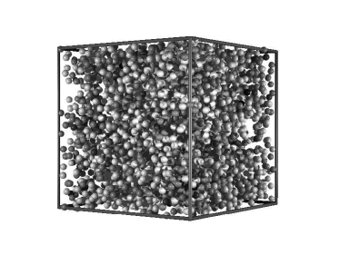
a) b)

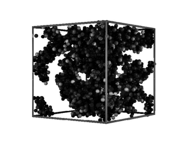
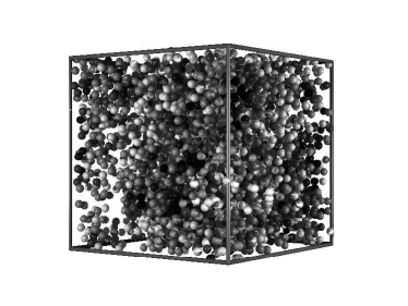
c) d)

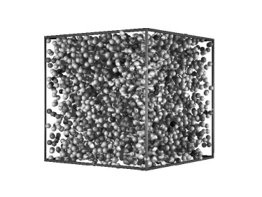
Figure 2: Memory effects in a steered simulation: the grayscale denotes the coordination number. Particles closer than 2.4 radii are considered to be neighbors. Dark particles in this sense are highly coordinated, bright ones have low coordination numbers. a) right after initialization, homogeneous distribution of the particles, b) cluster formation after tuning the potentials to be attractive, c) still inhomogeneous regions after steering the simulation out of the clustered region, d) the system is homogeneous again when diffusion has counterbalanced the density inhomogeneities. The steering path in the parameter space as well as the points a)–d) thereon are illustrated in Fig. 3.

Since several parameters, namely the volume fraction, $p\mathrm{H}$-value, ionic strength, external driving forces influence the system, a first step to understand its behavior is to examine it in the absence of external forces. Still, two parameters–the $p\mathrm{H}$-value and the ionic strength–govern the dynamics of the system. If the potentials are attractive, cluster formation can be observed Hecht et al. (2007b), provided the attraction is strong enough compared to thermal fluctuations. In our previous work Hecht et al. (2007a); Hecht (2007) we have explored this part of the parameter space for some distinct volume fractions by running numerous individual simulations. However, with the newly implemented steering approach one can detect boundaries between different regions of the stability diagram faster and more sensitively.

In Fig. 2 we illustrate the effects of changing the properties of the interaction potentials. All the snapshots belong to the same simulation and represent different points of the trajectory the system is steered through parameter space: a) The initial situation with repulsive potentials, shortly after initialization of the system, b) after crossing the boundary to the clustered region, c) shortly after steering back to the suspended regime, where still some inhomogeneities in the system can be observed, and finally d) after some time when diffusion has restored a homogeneous system. This time depends on the distances between the clusters and on the characteristic diffusion time of the particles. The steering path in the configuration space is shown in Fig. 3. The points at which the snapshots of Fig. 2 are taken, are marked by black dots. In the insets in Fig. 3 the total potential is plotted for several cases. During the simulation we change the $p\mathrm{H}$-value and the ionic strength and we drive the system along a closed trajectory in parameter space. We start at low ionic strength $I=1\,\mathrm{mmol/l}$ and $p\mathrm{H}=4$ (potential shown) and first increase the $p\mathrm{H}$-value (potential shown for $I=1\,\mathrm{mmol/l}$ and $p\mathrm{H}=7$), then increase the ionic strength, then reduce the $p\mathrm{H}$-value again while further increasing the ionic strength (potential shown for $I=15\,\mathrm{mmol/l}$ and $p\mathrm{H}=4$) and finally decrease the ionic strength to return to the starting point. We choose the trajectory such that the barrier between the primary and the more shallow, secondary minimum of the DLVO potential does not go below 5 $k_{\mathrm{B}}T$. Since the secondary minimum becomes deeper during the simulation cluster formation can be observed. However, the barrier between the primary and the secondary minimum of the DLVO potentials prevents irreversible aggregation in the primary minimum. A case in which the barrier vanishes and irreversible aggregation would appear is also shown in the upper right inset ($I=15\,\mathrm{mmol/l}$ and $p\mathrm{H}=7$). In any case, in our simulation all clusters dissolve again after steering back to a lower $p\mathrm{H}$-value and lower ionic strength (see Fig. 2 d)). This confirms that we have reversible clustering in the secondary minimum of the DLVO potentials.

One of the advantages of a steered simulation is, that one can more accurately detect the onset of the cluster formation than by starting individual simulations for different conditions. One might predict the boundary by evaluating the depth of the secondary minimum in the potential, but since also the hydrodynamic damping forces and an eventually applied driving pressure influence this process the prediction of the boundary can become more complicated. We have experienced similar difficulties in the context of shear flow simulations of the same colloidal suspension Hecht et al. (2006, 2007a).

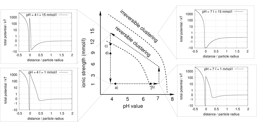
Figure 3: Steering path of the simulation: we start at the bottom left corner at low $p\mathrm{H}$-value and low ionic strength and steer the simulation along the dashed path through parameter space. The region of reversible cluster formation is reached, but the barrier between primary and secondary minimum of the DLVO potentials prevents irreversible clustering: when reaching the starting point again, all clusters have vanished. The boundary of the clustering region is sketched: Reversible clustering is observed when the depth of secondary DLVO minimum is in the order of $k_{\mathrm{B}}T$ and irreversible clustering appears when the height of the barrier between the two DLVO minima is of the order of $k_{\mathrm{B}}T$ or less. The labeled black dots mark the positions at which the snapshots of Fig. 2 are taken. The insets show the total potential at some selected extreme cases (see text).

A quantity to support the visualization of clusters is the coordination number. We consider two particles whose centers are closer than $2.4$ particle radii as neighbors and define the coordination number of each particle as the number of its neighbors in the sense just described. The particles in Fig. 2 are drawn in a grayscale corresponding to their coordination number, where dark particles are highly coordinated particles and bright ones are those with a low coordination number. At the beginning of the simulation (top left) the particles are distributed homogeneously over the whole simulation volume. After steering the simulation in the parameter space into the region of attractive potentials, cluster formation can be observed (top right). When the potentials are made less attractive again, the clusters dissolve (bottom left). However, the particles preferably stay at their positions and thus, the inhomogeneities in the system do not disappear immediately, which can be seen also in the dark color denoting high coordination numbers. After some time, diffusion restores the homogeneity of the system (bottom right). However, if the $p\mathrm{H}$-value or the ionic strength is increased too much, so that the barrier between the primary and the secondary minimum of the DLVO potentials vanishes, the clustering process becomes irreversible, which we avoided by the choice of the steering path (Fig. 3).

In this example the simulation remembers the interaction by the user. Even if the steering path is selected carefully inside the reversible range, the simulated suspension needs a characteristic time to relax after changing the interactions. The interaction by the user can be seen as a perturbation in the physical sense and the system needs time to adopt to the new situation. In these cases special care is advised when steering a simulation. We illustrate this by another example in the following subsection.

III.3 sedimentation: hydrodynamic interaction

Figure 4: Sedimentation velocity of a $\Phi=5\%$ suspension in a closed vessel. The sedimentation velocity of the particles in the upper part of the system is averaged over several time steps. The particles at the bottom of the system are not encountered. The velocity depends on the particle-particle interaction. Clusters settle down faster than individual particles. Symbols denote simulation results, the line is a guide to the eye.

Not only the particle positions and velocities, but also hydrodynamic interactions can influence the behavior of the system. Therefore, inhomogeneous particle distributions induced by steering the simulation first into a clustered region of the parameter space before simulating a different situation, might influence the result: we show in the following paragraph that a sedimentation process can happen faster, if cluster formation by attractive interactions creates density inhomogeneities in the system.

The friction force a single particle feels in a sedimentation process can be calculated analytically, but it differs if other particles are present. In LABEL:Hecht05 we have confirmed that the sedimentation velocity in our simulation depends on the volume fraction, as it is well-known from sedimentation theory Richardson and Zaki (1954). But even at constant volume fraction the sedimentation velocity can be different in different configurations. If the particles form clusters, the whole cluster settles down and the fluid streams around the whole cluster. The resistance is much less compared to the case when the particles are distributed homogeneously and the fluid streams around each of them separately (compare LABEL:Hecht07 and references therein). In Fig. 4 we have plotted the sedimentation velocity evaluated in several simulations, which only differ by the potentials. The volume fraction is the same for all of them. However, as one can see in the figure, the sedimentation velocity is smaller for low $p\mathrm{H}$-values.

This can be explained as follows: Since for increasing $p\mathrm{H}$-value the potentials become attractive, the particles form clusters and settle down faster. This effect is purely due to the hydrodynamics of the system. Since the streaming field depends on all particle positions and velocities not only at a given time, but also on their history, steering in this context may be very dangerous. When long range interactions, like hydrodynamics, which also depends on the history of the system, is important, steering should be avoided. In this case, to obtain reasonable results, one has to start again from an initial configuration when changing the interactions.

IV Conclusion

Bearing in mind the underlying physics, one can roughly estimate the limits of steered simulations. Let us summarize the points we have brought forward in this paper. First of all, steering can save computing time when aiming at a rough understanding of the influences on a system, especially when looking for the “interesting points” in parameter space, e.g., when searching for transition lines between different phases. We have shown this by the onset of cluster formation due to modifying the interaction potentials in a model suspension. Steering can be used as well to start data acquisition after a transient at the beginning of a simulation or to adjust the frequency for the data acquisition according to the current state of the simulation. This is especially interesting for large simulations with long transient times, as illustrated by the example of filter flow. We also explained why in some cases steering may be seen as a perturbation of the system, especially when the interaction potentials are changed. Special care is advised when dealing with non ergodic systems, memory effects, or long range interactions, like the role of hydrodynamics in sedimentation in our last example.

References

- Ladd (1994a) A. J. C. Ladd, J. Fluid Mech. 271, 285 (1994a).
- Ladd (1994b) A. J. C. Ladd, J. Fluid Mech. 271, 311 (1994b).
- Phung et al. (1996) T. N. Phung, J. F. Brady, and G. Bossis, J. Fluid Mech. 313, 181 (1996).
- L. E. Silbert et al. (1997) L. E. Silbert, J. R. Melrose, and R. C. Ball, Phys. Rev. E 56, 7067 (1997).
- Harnau and Dietrich (2004) L. Harnau and S. Dietrich, Phys. Rev. E 69, 051501 (2004).
- Vervey and Overbeek (1948) E. J. W. Vervey and J. T. G. Overbeek, Theory of the Stability of Lyophobic Colloids (Elsevier, Amsterdam, 1948).
- Derjaguin and Landau (1941) B. V. Derjaguin and L. D. Landau, Acta Physicochimica USSR 14, 633 (1941).
- Alexander et al. (1984) S. Alexander, P. M. Chaikin, P. Grant, G. J. Morales, P. Pincus, and D. Hone, J. Chem. Phys. 80, 5776 (1984).
- Grimson and Silbert (1991) M. J. Grimson and M. Silbert, Molecular Physics 74, 397 (1991).
- van Roij and Hansen (1997) R. van Roij and J.-P. Hansen, Phys. Rev. Lett. 79, 3082 (1997).
- Dobnikar et al. (2003) J. Dobnikar, Y. Chen, R. Rzehak, and H. H. von Grünberg, J. Phys.: Condens. Matter 15, S263 (2003).
- Trappe et al. (2001) V. Trappe, V. Prasad, L. Cipelletti, P. N. Segre, and D. A. Weitz, Nature 411, 772 (2001).
- Levin et al. (2003) Y. Levin, T. Trizac, and L. Bocquet, J. Phys.: Condens. Matter 15, S3523 (2003).
- Costa et al. (2005) D. Costa, J.-P. Hansen, and L. Harnau, Mol. Phys. 103, 1917 (2005).
- Hynninen et al. (2004) A.-P. Hynninen, M. Dijkstra, and R. van Roij, Phys. Rev. E 69, 061407 (2004).
- de Candia et al. (2005) A. de Candia, E. del Gado, A. Fierro, N. Sator, and A. Coniglio, Physica A 358, 239 (2005).
- Hütter (1999) M. Hütter, Ph.D. thesis, Swiss Federal Institute of Technology Zurich (1999), URL http://e-collection.ethbib.ethz.ch/cgi-bin/show.pl?type=diss&%nr=13107.
- Graule et al. (1994) T. J. Graule, F. H. Baader, and L. J. Gauckler, ceramic forum international 71, 314 (1994).
- Graule et al. (1995) T. J. Graule, F. H. Baader, and L. J. Gauckler, CHEMTECH 25, 31 (1995).
- Mallamace et al. (2006) F. Mallamace, S. H. Chen, A. Coniglio, L. de Arcangelis, E. Del Gado, and A. Fierro, Phys. Rev. E 73, 020402(R) (2006).
- Graf and Löwen (1998) H. Graf and H. Löwen, Phys. Rev. E 57, 5744 (1998).
- Hecht et al. (2007a) M. Hecht, J. Harting, and H. J. Herrmann, Phys. Rev. E 75, 051404 (2007a).
- Linse (2000) P. Linse, J. Chem. Phys. 113, 4359 (2000).
- Hecht et al. (2006) M. Hecht, J. Harting, M. Bier, J. Reinshagen, and H. J. Herrmann, Phys. Rev. E 74, 021403 (2006).
- Prins et al. (1999) J. Prins, J. Hermans, G. Mann, L. Nyland, and M. Simons, Future Generation Computer Systems 15, 485 (1999).
- Chin et al. (2003) J. Chin, J. Harting, S. Jha, P. Coveney, P. A.R., and S. Pickles, journal Contemporary Physics 44, 417 (2003).
- Hecht et al. (2005) M. Hecht, J. Harting, T. Ihle, and H. J. Herrmann, Phys. Rev. E 72, 011408 (2005).
- Hecht (2007) M. Hecht, Ph.D. thesis, Universität Stuttgart, Germany (2007), URL http://elib.uni-stuttgart.de/opus/volltexte/2007/2965/.
- Oberacker et al. (2001) R. Oberacker, J. Reinshagen, H. von Both, and M. J. Hoffmann, in Ceramic Processing Science VI, edited by N. C. S. Hirano, G.L. Messing (acers, 2001), vol. 112, pp. 179–184, iSBN 1574981048.
- Richter and Huber (2003) S. Richter and G. Huber, Granular Matter 5, 121 (2003).
- Kalthoff et al. (1996) W. Kalthoff, S. Schwarzer, G. Ristow, and H. J. Hermann, Int. J. Mod. Phys. C 7, 543 (1996).
- Kalthoff et al. (1997) W. Kalthoff, S. Schwarzer, and H. J. Herrmann, Phys. Rev. E 56, 2234 (1997).
- Wachmann et al. (1998) B. Wachmann, W. Kalthoff, S. Schwarzer, and H. J. Herrmann, Granular Matter 1, 75 (1998).
- Schwarzer (1995) S. Schwarzer, Phys. Rev. E 52, 6461 (1995).
- Brady and Bossis (1988) J. F. Brady and G. Bossis, Ann. Rev. Fluid Mech. 20, 111 (1988).
- Brady (1993) J. F. Brady, J. Chem. Phys. 99, 567 (1993).
- Sierou and Brady (2001) A. Sierou and J. F. Brady, J. Fluid Mech. 448, 115 (2001).
- Sierou and Brady (2004) A. Sierou and J. F. Brady, J. Fluid Mech. 506, 285 (2004).
- Hütter (2000) M. Hütter, J. Colloid Interface Sci. 231, 337 (2000).
- Ladd and Verberg (2001) A. J. C. Ladd and R. Verberg, J. Stat. Phys. 104, 1191 (2001).
- Komnik et al. (2004) A. Komnik, J. Harting, and H. J. Herrmann, Journal of Statistical Mechanics: theory and experiment P12003 (2004).
- Inoue et al. (2002) Y. Inoue, Y. Chen, and H. Ohashi, J. Stat. Phys. 107, 85 (2002).
- Padding and Louis (2004) J. T. Padding and A. A. Louis, Phys. Rev. Lett. 93, 220601 (2004).
- Malevanets and Kapral (1999) A. Malevanets and R. Kapral, J. Chem. Phys. 110, 8605 (1999).
- Malevanets and Kapral (2000) A. Malevanets and R. Kapral, J. Chem. Phys. 112, 7260 (2000).
- Ripoll et al. (2004) M. Ripoll, K. Mussawisade, R. G. Winkler, and G. Gompper, Europhys. Lett. 68, 106 (2004).
- Winkler et al. (2004) R. G. Winkler, K. Mussawisade, M. Ripoll, and G. Gompper, J. Phys.: Condens. Matter 16, S3941 (2004).
- Ali et al. (2004) I. Ali, D. Marenduzzo, and J. M. Yeomans, J. Chem. Phys. 121, 8635 (2004).
- Ripoll et al. (2005) M. Ripoll, K. Mussawisade, R. G. Winkler, and G. Gompper, Phys. Rev. E 72, 016701 (2005).
- Ripoll et al. (2006) M. Ripoll, R. G. Winkler, and G. Gompper, Phys. Rev. Lett. 96, 188302 (2006).
- Ihle and Kroll (2003a) T. Ihle and D. M. Kroll, Phys. Rev. E 67, 066705 (2003a).
- Ihle and Kroll (2003b) T. Ihle and D. M. Kroll, Phys. Rev. E 67, 066706 (2003b).
- Padding and Louis (2006) J. T. Padding and A. A. Louis, Phys. Rev. E 74, 031402 (2006).
- Malevanets and Yeomans (2000) A. Malevanets and J. M. Yeomans, Europhys. Lett. 52, 231 (2000).
- Falck et al. (2004) E. Falck, J. M. Lahtinen, I. Vattulainen, and T. Ala-Nissila, Eur. Phys. J. E 13, 267 (2004).
- Tuzel et al. (2003) E. Tuzel, M. Strauss, T. Ihle, and D. M. Kroll, Phys. Rev. E 68, 036701 (2003).
- Hecht et al. (2007b) M. Hecht, J. Harting, and H. J. Herrmann, Int. J. Mod. Phys. C 18, 501 (2007b).
- Richardson and Zaki (1954) J. F. Richardson and W. N. Zaki, Trans. Instn. Chem. Engrs. 32, 35 (1954).