Quantum to Classical Transition of the Charge Relaxation Resistance
of a Mesoscopic Capacitor

Abstract

We present an analysis of the effect of dephasing on the single channel charge relaxation resistance of a mesoscopic capacitor in the linear low frequency regime. The capacitor consists of a cavity which is via a quantum point contact connected to an electron reservoir and Coulomb coupled to a gate. The capacitor is in a perpendicular high magnetic field such that only one (spin polarized) edge state is (partially) transmitted through the contact. In the coherent limit the charge relaxation resistance for a single channel contact is independent of the transmission probability of the contact and given by half a resistance quantum. The loss of coherence in the conductor is modeled by attaching to it a fictitious probe, which draws no net current. In the incoherent limit one could expect a charge relaxation resistance that is inversely proportional to the transmission probability of the quantum point contact. However, such a two terminal result requires that scattering is between two electron reservoirs which provide full inelastic relaxation. We find that dephasing of a single edge state in the cavity is not sufficient to generate an interface resistance. As a consequence the charge relaxation resistance is given by the sum of one constant interface resistance and the (original) Landauer resistance. The same result is obtained in the high temperature regime due to energy averaging over many occupied states in the cavity. Only for a large number of open dephasing channels, describing spatially homogenous dephasing in the cavity, do we recover the two terminal resistance, which is inversely proportional to the transmission probability of the QPC. We compare different dephasing models and discuss the relation of our results to a recent experiment.

I Introduction

Interest in quantum coherent electron transport in the AC regime has been revived recently thanks to progress made in controlling and manipulating small high mobility mesoscopic structures driven by high frequency periodic voltages at ultra low temperatures. The state of the art includes the realization of high frequency single electron sources, which might be important for metrology. In Ref. Fève et al., 2007 this was achieved by applying large amplitude periodic voltage pulses of a few hundred MHz on the gate of a mesoscopic capacitor. The accuracy of this single electron emitter was analyzed theoretically in Ref. Moskalets et al., 2007. In Ref. Kataoka et al., 2007, pulses of surface acoustic waves were used to transport electrons one by one on a piezoelectric GaAs substrate. Two parameter quantized pumping with localized electrical potentials has been demonstrated in Ref. Blumenthal et al., 2007 and one parameter non-adiabatic quantized charge pumping in Ref. Kaestner et al., 2007. These experiments use frequencies in the GHz range to control the population and depopulation of one (or several) localized level(s). Thus the dynamics of charge relaxation is of central importance for these experiments.

Of particular interest to us here is the work of Gabelli et al. Gabelli et al. (2006), who succeeded in measuring both the in and out of phase parts of the linear AC conductance $G(\omega)=I(\omega)/V(\omega)$ of a mesoscopic capacitor at the driving frequency $\omega\approx 1\,{\rm GHz}$. The capacitor consists of a sub-micrometer Quantum Dot (QD) connected to an electron reservoir via a tunable Quantum Point Contact (QPC) and capacitively coupled to a metallic back or top gate (see Fig. 1).

The question “What is the RC-time of a quantum coherent capacitor?” has been theoretically addressed by Büttiker, Thomas and Prêtre Büttiker et al. (1993a). In the low frequency regime $\omega\ll 1/\tau_{RC}$, where $\tau_{RC}$ is the RC-time of the system, the response is determined by an electrochemical capacitance $C_{\mu}$ and a charge relaxation resistance $R_{q}$.

\psfrag{Vqpc}[1.2]{$V_{QPC}$}\psfrag{1l}[l][1.2]{$V(\omega)$}\psfrag{phi}[l][1.2]{$V_{\phi}(\omega)$}\psfrag{1}{$\color[rgb]{0,0,1}{N_{1}}$}\psfrag{N}[r]{$N_{\phi}$}\psfrag{Nm1}[r]{$N_{\phi}-1$}\psfrag{Vg}[1.2]{$V_{g}$}\psfrag{U}[1.2]{$U(\omega)$}\psfrag{C}{$C$}\psfrag{e}{$\color[rgb]{1,0,0}\varepsilon$}\psfrag{T}[1.4]{$\color[rgb]{0,0,1}\mathcal{T}$}\includegraphics[width=173.44534pt]{fig1.eps}

Figure 1: (Color online) Mesoscopic Capacitor. The full blue curve represents the current carrying channel connected to the reservoir via the QPC while the dashed dotted black curves represent additional localized states, disconnected from the reservoir. As an example, the innermost edge state (highest Landau Level) is here split into three localized states illustrating the possibility of having more than one localized state per Landau Level. The red dashed lines represent incoherent scattering between states in the cavity. $\mathcal{T}$ is the transmission probability of the QPC and $\varepsilon$ is the inter-channel coupling strength. $U(\omega)$ is the Fourier transform of the time-dependent electric potential $U(t)$ inside the cavity. The functions of the various voltages are discussed in the text.

Together these determine the RC-time in complete analogy to the classical case: $\tau_{RC}=R_{q}C_{\mu}$ . These two quantities however differ fundamentally from their classical counterparts. In particular the quantum RC-time obtained from their product, is sensitive to the quantum coherence of the system and consequently displays typical mesoscopic fluctuations Gopar et al. (1996); Brouwer and Büttiker (1997); Brouwer et al. (1997); Büttiker and Nigg (2007). For a system, with many conducting channels Brouwer and Büttiker (1997), these fluctuations are present separately in both the capacitance and the resistance. Surprisingly, for a coherent capacitor with a single channel, only the capacitance fluctuates and the resistance is found to be constant and given by half a resistance quantum Büttiker et al. (1993b)

$$R_{q}=\frac{h}{2e^{2}}\,.$$ (1)

This quantization has indeed been observed experimentally Gabelli et al. (2006) thus establishing a novel manifestation of quantum coherence in the AC regime.

The claim that the quantization of $R_{q}$ requires quantum coherence is perhaps not so astonishing. The interesting question is the length scale on which coherence is necessary. For the integer quantized Hall effect von Klitzing et al. (1980) coherence is necessary only over a cyclotron radius which is sufficient to establish a Landau level structure. In fact as discussed in Ref. Büttiker, 1988a inelastic scattering (the destruction of long range coherence) can even help to establish quantization of the Hall resistance. Similarly in quantum point contacts van Wees et al. (1988); Wharam et al. (1988) coherence over the width of the conduction channel is in principle sufficient to establish a step-like structure of the conductance. In contrast, as we will show, the quantization of the charge relaxation resistance requires coherence over the entire capacitance plate (the quantum dot) and not only over the contact region. Thus the quantized charge relaxation resistance in Eq. (1) is indeed very sensitive to dephasing.

There is a second important aspect in which the quantized charge relaxation resistance $R_{q}=h/(2e^{2})$ differs from quantization of a Hall resistance von Klitzing et al. (1980) or of a ballistic conductance van Wees et al. (1988); Wharam et al. (1988). In both of these latter cases quantization is associated with perfect transmission channels which permit unidirectional electron motion through the sample. In contrast, the quantization of $R_{q}$ is independent of the transmission probability of the contact! For a coherent capacitor plate connected via a single spin polarized channel to a reservoir the quantization of $R_{q}$ is truly universal and holds even in the Coulomb blockade regime Nigg et al. (2006).

Of course, no matter how pure the samples are, a spurious interaction of the system with environmental degrees of freedom, is unavoidable. This introduces dephasing into the system.

It is thus of interest to ask how dephasing affects the quantization of the single channel charge relaxation resistance and to investigate the crossover from the coherent to the incoherent regime. Furthermore, in typical measurements the temperature, though low compared with the level spacing of the sample, is still comparable to other relevant energy scales such as the driving frequency or the coupling strength between cavity and lead. From a theoretical point of view it is thus desirable to be able to distinguish between thermal averaging and effects due to pure dephasing and to understand the interplay between these two fundamental mechanisms. Intuitively, one would expect that in the presence of strong enough dephasing, the QD starts behaving like an electron reservoir and thus that a fully incoherent single channel capacitor should exhibit the two terminal resistance

$$R_{q}=\frac{h}{e^{2}}\frac{1}{\mathcal{T}},$$ (2)

where $\mathcal{T}$ is the transmission probability of the channel through the QPC connecting the system to the electron reservoir. Interestingly, neither dephasing nor energy averaging (high-temperature limit) lead directly to Eq. (2). We find that for the QD to become a true electron reservoir it is necessary that many channels participate in the inelastic relaxation process which a true reservoir must provide.

In the present work we employ a description of dephasing provided by the voltage and dephasing probe models Büttiker (1986, 1988b); Datta and Lake (1991); de Jong and Beenakker (1996); Pilgram et al. (2006), where one attaches a fictitious probe to the system which can absorb and re-emit electrons from or into the conductor. If the probe supports only one channel, we find that the charge relaxation resistance of the fully incoherent mesoscopic capacitor is given by

$$R_{q}=\frac{h}{2e^{2}}+\frac{h}{e^{2}}\frac{1-\mathcal{T}}{\mathcal{T}}\,,$$ (3)

Hence, the charge relaxation resistance is given by the sum of the resistance as found from the (original) Landauer Landauer (1970) formula $h/e^{2}(1-\mathcal{T})/\mathcal{T}$ and one interface resistance Imry (1986); Landauer (1987) $h/(2e^{2})$. Incidentally, as we show below, this is also the value of $R_{q}$ obtained in the high temperature limit for the coherent system, illustrating an interesting relation between single channel dephasing and temperature induced phase averaging. A hybrid superconducting-normal conductor provides another geometry with only one normal narrow-wide interface Sols and Sanchez-Cañizares (1999).

In the next two sections, we introduce the physical system and the dephasing models. Then in section IV, we specialize our model to a specific form of the scattering matrix appropriate for transport along edge states of the integer quantum Hall regime and discuss the main results. Finally, our conclusions are given in section V.

II The mesoscopic capacitor

The system we consider can be viewed as the mesoscopic equivalent of the ubiquitous classical series RC circuit. One of the macroscopic “plates” of the classical capacitor is replaced by a QD and the role of the resistor is played by a QPC connecting this QD to an electron reservoir. This system is represented schematically in Fig. 1. The curves with arrows represent the transport channels of the system corresponding physically to edge states of the integer (spin polarized) quantum Hall regime, in which the experiment of Ref. Gabelli et al., 2006 was performed. By varying the gate voltage $V_{QPC}$, one changes both the transparency of the QPC and the electrostatic potential in the cavity. In the present work we take the gate voltage $V_{g}$, applied to the macroscopic “plate” of the capacitor, as a fixed voltage reference and set it to zero. A sinusoidal AC voltage $V(\omega)$, applied to the electron reservoir, drives an AC current through the system.

The low frequency linear AC response of the mesoscopic capacitor can be characterized Büttiker et al. (1993a) by an electrochemical capacitance $C_{\mu}$ and a charge relaxation resistance $R_{q}$, defined via the AC conductance as

$$G(\omega)=-i\omega C_{\mu}+\omega^{2}C_{\mu}^{2}R_{q}+O(\omega^{3})\,.$$ (4)

The linear low frequency regime is given by $eV_{ac}\ll\hbar\omega\ll\Delta$, where $V_{ac}$ is the amplitude of the AC voltage and $\Delta$ is the mean level spacing in the QD.

Even in very clean samples some coupling of the current carrying edge channel to some environmental states is unavoidable. For example, we can expect that an electron entering the QD in the current carrying edge channel (full blue curve in Fig. 1) may be scattered (red dashed lines in Fig. 1) by phonons or other electrons into localized states belonging to other (higher) Landau levels not directly connected to the lead, before being scattered back into the open edge channel and returning to the electron reservoir. If on the one hand, this inter-edge state scattering is purely elastic, the presence of these closed states is known to lead to a periodic modulation of the conductance as a function of gate voltage, the period of which is proportional to the number of closed states Staring et al. (1992); Heinzel et al. (1994). Such modulations, with a period corresponding to about $10$ to $15$ closed states, have indeed been observed in the experiment of Ref. Gabelli et al., 2006 at low temperatures for a magnetic field strength of $1.3\,{\rm T}$. If on the other hand the scattering is inelastic, such processes will in general be incoherent, i.e. they will destroy the information carried by the phase of the electronic wave and hence lead to dephasing.

The idea of the present work is to mimic the latter processes using the voltage and dephasing probe models as illustrated in Fig. 2. The extension of these models to the AC regime is presented in the next section. For simplicity, we will here neglect the contribution of the elastic processes and focus solely on the inelastic ones.

III Voltage and dephasing probe models in the AC regime

\psfrag{VQPC}[1.2]{$V_{QPC}$}\psfrag{V}[l][1.2]{$V(\omega)$}\psfrag{phi}[l][1.2]{$V_{\phi}(\omega)$}\psfrag{1}{$\color[rgb]{0,0,1}{N_{1}}$}\psfrag{N}[r]{$N_{\phi}$}\psfrag{Nm1}[r]{$N_{\phi}-1$}\psfrag{Vg}[1.2]{$V_{g}$}\psfrag{U}[l][l][1]{$U(\omega)$}\psfrag{C}{$C$}\psfrag{DPVP}{DP, VP}\psfrag{e}{$\color[rgb]{1,0,0}\varepsilon$}\psfrag{T}[0.9]{$\color[rgb]{0,0,1}\mathcal{T}$}\psfrag{Ip}[1]{$I_{\phi}=0$}\psfrag{DPVP}{DP or VP, $I_{\phi}=0$}\includegraphics[width=164.77771pt]{fig2.eps}

Figure 2: (Color online) Schematic representation of the voltage and dephasing probe models. The incoherent inter-channel coupling depicted in Fig. 1, is mediated by a Voltage Probe (VP) or a Dephasing Probe (DP) represented as a shaded plane. The entire system including the fictitious probe, which draws no net current, is again described as a coherent multi-terminal scatterer.

To simulate the loss of phase coherence of electrons inside the cavity, we attach to the quantum dot a fictitious probe Büttiker (1986, 1988b); Datta and Lake (1991); de Jong and Beenakker (1996), which draws no net current. An electron entering this probe is immediately replaced by an electron re-injected incoherently into the conductor. The main advantage of this approach is that the entire system consisting of the conductor and the probe can be treated as a coherent multi-terminal conductor within the scattering matrix approach. Some recent applications of this approach include investigations on the effect of dephasing on quantum pumping Moskalets and Büttiker (2001); Chung et al. (2007), on quantum limited detection Clerk and Stone (2004) and on photon assisted shot noise Polianski et al. (2005). The effect of dephasing on shot noise and higher moments (counting statistics) has been investigated in Refs. Pilgram et al., 2006 and Förster et al., 2007. A probe which dephases spin states has been introduced in Ref. Michaelis and Beenakker, 2006.

In terms of the spectral current density $i_{\alpha}(E,\omega)$, the current at the driving frequency $\omega$ into probe $\alpha$ is expressed as

$$I_{\alpha}(\omega)=\int dE\,i_{\alpha}(E,\omega)\,.$$ (5)

The gauge invariant spectral current in turn is given by

$$i_{\alpha}(E,\omega)=\sum_{\beta}g_{\alpha\beta}(E,\omega)(V_{\beta}(\omega)-U(\omega))\,,$$ (6)

where

$$g_{\alpha\beta}(E,\omega)=\frac{e^{2}}{h}F_{\beta}(E,\omega){\rm tr}[\openone_{\alpha}\delta_{\alpha\beta}-S^{\dagger}_{\alpha\beta}(E)S_{\alpha\beta}(E+\hbar\omega)]$$ (7)

is the (unscreened) spectral AC conductance from probe $\beta$ to probe $\alpha$ and $F_{\beta}(E,\omega)=[f_{\beta}(E)-f_{\beta}(E+\hbar\omega)]/\hbar\omega$, $f_{\beta}$ being the electron distribution function in probe $\beta$. $V_{\beta}(\omega)$ is the voltage applied to reservoir $\beta$ and $U(\omega)$ is the Fourier transform of the electric potential inside the QD, which is assumed to be homogeneous. The inclusion of this potential, which accounts for the screening interaction between charges on the conductor and charges on the gate electrode, is essential to ensure gauge invariance in the dynamical regime Büttiker et al. (1993a). Finally, $S_{\alpha\beta}(E)$ is the $(N_{\alpha}+N_{\beta})\times(N_{\alpha}+N_{\beta})$ scattering matrix for electrons with energy $E$ scattered from the $N_{\beta}$ channels of probe $\beta$ to the $N_{\alpha}$ channels of probe $\alpha$.

In the following we will be interested in the situation where only one current carrying channel (full blue curve in Fig. 2) connects the QD to the electron reservoir ($N_{1}=1$), while the number of channels coupling to the fictitious probe $N_{\phi}$ is arbitrary.

For the voltage probe, we require that the current into the fictitious probe vanishes at each instant of time or equivalently at all frequencies, i.e. $I_{\phi}(\omega)=0$. For the dephasing probe, we require in addition that the current into the probe vanishes in any infinitesimal energy interval $dE$ and thus that the spectral current $i_{\phi}(E,\omega)=0$. This latter condition simulates quasi-elastic scattering where the energy exchanged is small compared to all other energy scales. Clearly, with these definitions, a dephasing probe is also a voltage probe but a voltage probe need not be a dephasing probe. In both cases however, current conservation implies that $I(\omega)\equiv I_{1}(\omega)=-i\omega CU(\omega)$, where $C$ is the geometrical capacitance of the QD. This relation, together with Eqs. (5) and (6), allows us to self-consistently eliminate the internal potential $U(\omega)$ in the usual fashion Büttiker et al. (1993a).

III.1 Voltage probe

From the condition $I_{\phi}(\omega)=0$, we find the AC conductance

$$G(\omega)=\frac{I(\omega)}{V(\omega)}=\frac{-i\omega C\chi(\omega)}{\chi(\omega)-i\omega C}\,,$$ (8)

where

$$\chi(\omega)=g_{11}(\omega)-\frac{g_{1\phi}(\omega)g_{\phi 1}(\omega)}{g_{\phi\phi}(\omega)}\,.$$ (9)

Here and for all of the following, we have introduced the notation $g_{\alpha\beta}(\omega)=\int dEg_{\alpha\beta}(E,\omega)$. Upon expanding to second order in $\omega$ and comparing coefficients with (4), we find

$$C_{\mu}=\frac{C\chi_{1}}{-iC+\chi_{1}}\quad\text{and}\quad R_{q}=-\frac{\chi_{2}}{{\chi_{1}}^{2}}\,,$$ (10)

with

$$\chi_{1}=\sum_{\alpha,\beta}g^{1}_{\alpha\beta}\,\,\,\text{and}\,\,\,\chi_{2}=\sum_{\alpha\beta}\Big{(}g^{2}_{\alpha\beta}-g^{1}_{\alpha\phi}g^{1}_{\phi\beta}/g^{0}_{\phi\phi}\Big{)}\,,$$ (11)

where $g_{\alpha\beta}(\omega)=g^{0}_{\alpha\beta}+g^{1}_{\alpha\beta}\omega+g^{2}_{\alpha\beta}\omega^{2}+O(\omega^{3})$ and $\chi(\omega)=\chi_{1}\omega+\chi_{2}\omega^{2}+O(\omega^{3})$. The conductance expansion coefficients are given in terms of the scattering matrix and its energy derivatives as

$$g_{\alpha\beta}^{i}=\int dEf_{\beta}^{\prime}(E)A_{\alpha\beta}^{i}(E)\,,\quad(i=1,2,3)$$ (12)

with

$$A_{\alpha\beta}^{0} =-\frac{e^{2}}{h}{\rm tr}[\openone_{\alpha}\delta_{\alpha\beta}-S^{\dagger}_{\alpha\beta}S_{\alpha\beta}]\,,$$

$$A_{\alpha\beta}^{1} =\frac{e^{2}}{4\pi}{\rm tr}[S_{\alpha\beta}^{\dagger}S_{\alpha\beta}^{\prime}-{(S_{\alpha\beta}^{\prime})^{\dagger}}S_{\alpha\beta}]\,,$$ (13)

$$A_{\alpha\beta}^{2} =-\frac{e^{2}h}{8\pi^{2}}{\rm tr}[{{S_{\alpha\beta}^{\prime}}^{\dagger}}S_{\alpha\beta}^{\prime}-\frac{1}{3}\left(S_{\alpha\beta}^{\dagger}S_{\alpha\beta}\right)^{\prime\prime}]\,,$$

where ^′ denotes differentiation with respect to $E$ and for compactness we have suppressed the energy arguments. In the voltage probe model the electrons in the fictitious lead are allowed to relax towards equilibrium arbitrarily fast and we thus have $f_{\phi}(E)=f_{1}(E)=1/[1+\exp(\beta(E-E_{F}))]\equiv f(E)$.

III.2 Dephasing probe

In contrast to the voltage probe, the distribution function $f_{\phi}(E)$ of the dephasing probe is a priori not known. The requirement $i_{\phi}(E,\omega)=0$, together with Eq. (6) yields

$$G(\omega)=\frac{-i\omega C\tilde{\chi}(\omega)}{\tilde{\chi}(\omega)-i\omega C}\,,$$ (14)

where

$$\tilde{\chi}(\omega)\equiv g_{11}(\omega)-\int dE\frac{g_{1\phi}(E,\omega)g_{\phi 1}(E,\omega)}{g_{\phi\phi}(E,\omega)}\,.$$ (15)

The electrochemical capacitance and the charge relaxation resistance are given in terms of the first and second order frequency expansion coefficients $\tilde{\chi}_{1}$ and $\tilde{\chi}_{2}$ as

$$C_{\mu}=\frac{C\tilde{\chi}_{1}}{-iC+\tilde{\chi}_{1}}\quad\text{and}\quad R_{q}=-\frac{\tilde{\chi}_{2}}{{\tilde{\chi}_{1}}^{\ 2}}\,.$$ (16)

Making use of the unitarity of the scattering matrix, we find explicitly

$$\tilde{\chi}_{1}=\sum_{\alpha\beta}\int dEf^{\prime}(E)A_{\alpha\beta}^{1}(E)=\chi_{1}\,,$$ (17)

and

$$\tilde{\chi}_{2}=\sum_{\alpha\beta}\left(g_{\alpha\beta}^{2}-\int dEf^{\prime}(E)\frac{A_{\alpha\phi}^{1}(E)A_{\phi\beta}^{1}(E)}{A_{\phi\phi}^{0}(E)}\right)\,.$$ (18)

Comparing with Eqs. (11), we see that at zero temperature, voltage and dephasing probes equally affect the AC conductance. At finite temperature, the electrochemical capacitance of the mesoscopic capacitor does still not distinguish between dephasing and voltage probes, while the charge relaxation resistance is in principle sensitive to whether the dephasing mechanism is quasi-elastic (dephasing probe) or inelastic (voltage probe).

IV Interfering edge state model

IV.1 Scattering matrix for independent channels

We next apply the two dephasing models described in the previous section to a model for the scattering matrix of the mesoscopic capacitor in the integer quantum Hall regime introduced in Refs. Gabelli et al., 2006 and Prêtre et al., 1996, which is here extended to include a voltage (dephasing) probe. The special form of the scattering matrix arises due to multiple reflections of the electronic wavefunction within the cavity in close analogy with a Fabry-Perot interferometer.

The additional probe, with $N_{\phi}$ channels is coupled to the single edge channel propagating through the QPC. Clearly $N_{\phi}-1$ channels of the probe are perfectly reflected at the QPC from within the cavity as depicted in Figs. 2 and 3. For simplicity, we shall assume the channels to be independent, which means that we consider the physical edge channels to coincide with the eigen-channels of the transmission matrix. Furthermore, we consider a symmetric QPC and assume that each channel couples identically to the fictitious probe with strength $\varepsilon$. Then the $(N_{\phi}+1)\times(N_{\phi}+1)$ scattering matrix $S_{1}$ of the QPC and the $2N_{\phi}\times 2N_{\phi}$ scattering matrix $S_{\varepsilon}$ of the fictitious probe have block diagonal form and may be parameterized as follows

$$S_{1}=\begin{pmatrix}r_{1}&t^{\prime}_{1}\\ t_{1}&r^{\prime}_{1}\end{pmatrix}\quad\text{and}\quad S_{\varepsilon}=\begin{pmatrix}r_{\varepsilon}&t^{\prime}_{\varepsilon}\\ t_{\varepsilon}&r^{\prime}_{\varepsilon}\end{pmatrix}$$ (19)

with $r_{1}=ir$ and $r^{\prime}_{1}={\rm diag}(ire^{i\phi_{1}(E)},e^{i\phi_{2}(E)},\dots$ $\dots,e^{i\phi_{N_{\phi}}(E)})$ where we take $r$ to be real and $\phi_{l}(E)$ is the phase accumulated by an electron during one round trip along the $l$-th edge state through the QD. $t_{1}=(\sqrt{1-r^{2}},0,\dots,0)^{T}$ and $t^{\prime}_{1}=(\sqrt{1-r^{2}}e^{i\phi_{1}(E)},0,\dots,0)$. Finally $r^{(\prime)}_{\varepsilon}={\rm diag}(i\sqrt{1-\varepsilon},\dots,i\sqrt{1-\varepsilon})$ and $t^{(\prime)}_{\varepsilon}={\rm diag}(\sqrt{\varepsilon},\dots,\sqrt{\varepsilon})$.

The total $(N_{\phi}+1)\times(N_{\phi}+1)$ scattering matrix, which is obtained from the series combination of the two scattering matrices $S_{1}$ and $S_{\varepsilon}$, takes the form

$$S=\begin{pmatrix}S_{11}&S_{1\phi}\\ S_{\phi 1}&S_{\phi\phi}\end{pmatrix}\,,$$ (20)

with

$$S_{11} =\frac{i(r+e^{i\phi_{1}}\sqrt{1-\varepsilon})}{1+re^{i\phi_{1}}\sqrt{1-\varepsilon}}\,,$$

$$S_{1\phi} =(\frac{\sqrt{\varepsilon(1-r^{2})}e^{i\phi_{1}}}{1+re^{i\phi_{1}}\sqrt{1-\varepsilon}},\overbrace{0,\dots,0}^{N_{\phi}-1})\,,$$ (21)

$$S_{\phi 1} =(\frac{\sqrt{\varepsilon(1-r^{2})}}{1+re^{i\phi_{1}}\sqrt{1-\varepsilon}},\overbrace{0,\dots,0}^{N_{\phi}-1})^{T}\,,$$

$$S_{\phi\phi} ={\rm diag}(\frac{i(\sqrt{1-\varepsilon}+re^{i\phi_{1}})}{1+re^{i\phi_{1}}\sqrt{1-\varepsilon}},\frac{i\sqrt{1-\varepsilon}+e^{i\phi_{2}}}{1-ie^{i\phi_{2}}\sqrt{1-\varepsilon}},\dots$$

$$\phantom{{\rm diag}(r^{\prime}_{\varepsilon_{1}}}\dots,\frac{i\sqrt{1-\varepsilon}+e^{i\phi_{N_{\phi}}}}{1-ie^{i\phi_{N_{\phi}}}\sqrt{1-\varepsilon}})\,.$$

\psfrag{S1}{$S_{1}$}\psfrag{S}{$S$}\psfrag{N}{$N_{\phi}$}\psfrag{1}{$1$}\psfrag{phi1}[0.7]{$\phi_{1}$}\psfrag{phi2}[0.7]{$\phi_{2}$}\psfrag{phi3}[0.7]{$\phi_{3}$}\psfrag{phi4}[0.7]{$\phi_{4}\dots$}\psfrag{S2}{$S_{\varepsilon}$}\includegraphics[width=173.44534pt]{fig3.eps}

Figure 3: (Color online) $S_{1}$ is the $(N_{\phi}+1)\times(N_{\phi}+1)$ scattering matrices of the QPC relating the incoming channel to the $N_{\phi}$ channels inside the cavity and $S_{\varepsilon}$ is the $2N_{\phi}\times 2N_{\phi}$ scattering matrix relating the $N_{\phi}$ channels in the cavity with the $N_{\phi}$ channels in the probe. From these two matrices one can derive $S$, the total scattering matrix relating the incoming channel to the $N_{\phi}$ channels in the probe. An electron in the $i$-th channel accumulates a phase $\phi_{i}$ inside the cavity.

Using these expressions together with (10) for the voltage probe, respectively (16) for the dephasing probe, we can express the electrochemical capacitance and the charge relaxation resistance as a function of the transparency $\mathcal{T}=1-r^{2}$ of the current carrying channel, the phases $\phi_{1},\dots,\phi_{N_{\phi}}$ and the coupling strength $\varepsilon$. In order to investigate the crossover from the coherent to the incoherent regime, we will later on make a specific physically motivated choice for the energy dependence of the phases. However, even without specifying the form of the energy-phase relation, we can already draw some general conclusions by looking at the incoherent limit $\varepsilon\rightarrow 1$. This we do next after briefly reviewing the coherent case $\varepsilon=0$.

IV.2 Results and discussion

IV.2.1 General results at zero temperature

We first consider the zero temperature limit. In this case voltage and dephasing probe models are equivalent as shown in section III. The capacitance and the resistance are given by

$$C_{\mu}=\frac{-C\sum_{\alpha\beta}A_{\alpha\beta}^{1}}{-iC-\sum_{\alpha\beta}A_{\alpha\beta}^{1}}\,,$$ (22)

and

$$R_{q}=\sum_{\alpha\beta}\left(A_{\alpha\beta}^{2}-\frac{A^{1}_{\alpha\phi}A^{1}_{\phi\beta}}{A^{0}_{\phi\phi}}\right)\Big{/}\left(\sum_{\alpha\beta}A_{\alpha\beta}^{1}\right)^{2}\,,$$ (23)

where $A^{i}_{\alpha\beta}\equiv A^{i}_{\alpha\beta}(E_{F})$ are given in Eq. (III.1). In the coherent regime ($\varepsilon=0$), we recover the universal result $R_{q}=h/(2e^{2})$ for the resistance while the capacitance is given by $C_{\mu}=Ce^{2}\nu/(C+e^{2}\nu)$, with the density of states of the cavity $\nu(E)=1/(2\pi i)S^{\dagger}(E)dS(E)/dE$, where $S(E)=\lim_{\varepsilon\rightarrow 0}S_{11}(E)$, for $S_{11}$ given in Eq. (IV.1). In the opposite, fully incoherent regime ($\varepsilon=1$), we find

$$C_{\mu}=\frac{C\frac{e^{2}}{2\pi}\sum_{i=1}^{N_{\phi}}\phi_{i}^{\prime}}{C+\frac{e^{2}}{2\pi}\sum_{i=1}^{N_{\phi}}\phi_{i}^{\prime}}\,,$$ (24)

which is independent of $\mathcal{T}$, and

$$R_{q}=\frac{h}{2e^{2}}\frac{\sum_{i=1}^{N_{\phi}}(\phi_{i}^{\prime})^{2}}{\left(\sum_{i=1}^{N_{\phi}}\phi_{i}^{\prime}\right)^{2}}+\frac{h}{e^{2}}\left(\frac{1}{\mathcal{T}}-\frac{\phi_{1}^{\prime}}{\sum_{i=1}^{N_{\phi}}\phi_{i}^{\prime}}\right)\,.$$ (25)

For a single open dephasing channel ($N_{\phi}=1$), Eq. (25) reduces to

$$R_{q}=\frac{h}{2e^{2}}+\frac{h}{e^{2}}\frac{1-\mathcal{T}}{\mathcal{T}}\,.$$ (26)

Thus, as mentioned in the introduction, if only the current carrying channel is dephased, the charge relaxation resistance is the sum of a constant interface resistance Imry (1986); Landauer (1987); Sols and Sanchez-Cañizares (1999) $R_{c}=h/(2e^{2})$ and the original Landauer resistance $R_{L}=h/e^{2}(1-\mathcal{T})/\mathcal{T}$ of the QPC.

IV.2.2 Smooth potential approximation

In the following, we will assume that the potential in the cavity is sufficiently smooth so that the energy dependent part of the accumulated phase is the same for all channels. Then $\phi_{1}^{\prime}\approx\phi_{2}^{\prime}\approx\dots\phi_{N_{\phi}}^{\prime}\equiv\phi^{\prime}$. Within this approximation, Eqs. (24) and (25) reduce to

$$C_{\mu}=\frac{C\frac{e^{2}}{2\pi}N_{\phi}\phi^{\prime}}{C+\frac{e^{2}}{2\pi}N_{\phi}\phi^{\prime}}\,,$$ (27)

and

$$R_{q}=\frac{h}{e^{2}}\frac{1-\mathcal{T}}{\mathcal{T}}+\frac{h}{2e^{2}}+\frac{h}{2e^{2}}\frac{N_{\phi}-1}{N_{\phi}}\,.$$ (28)

Written in this way, this expression for $R_{q}$ again lends itself to a simple interpretation. The first term on the righthand side of Eq. (28), is the original Landauer resistance of the QPC. The second term $R_{c}\equiv\frac{h}{2e^{2}}$ is the interface resistance of the real reservoir-conductor interface and the third term $R_{\phi}=\frac{h}{2e^{2}}\frac{N_{\phi}-1}{N_{\phi}}$ is the resistance contributed to by the dephasing. In the limit of a very large number of open dephasing channels ($\varepsilon=1,\ N_{\phi}\gg 1$), which corresponds physically to spatially homogeneous dephasing, $R_{\phi}\rightarrow R_{c}$ and so $R_{q}\rightarrow h/e^{2}(1/\mathcal{T})$ as well as $C_{\mu}\rightarrow C$. Thus, in this limit the fictitious probe contributes half a resistance quantum and the mesoscopic capacitor behaves like a classical RC circuit with a two terminal resistance in series with the geometrical gate capacitance.

Next we investigate the crossover from the coherent to the incoherent regime. For this purpose, we assume that the accumulated phase depends linearly on energy in the vicinity of the Fermi energy; explicitly we take $\phi_{1}(E)=\phi_{2}(E)=\dots=\phi_{N_{\phi}}(E)=2\pi E/\Delta$, where $\Delta$ is the mean level spacing in the cavity. Then, the fictitious probe is characterized by only two parameters; the number of channels $N_{\phi}$ and the coupling strength $\epsilon$. Following Ref. Büttiker, 1988b, the latter can be related to the dephasing time $\tau_{\phi}$. The scattering amplitudes have poles at the complex energies $E=E_{n}-i\Gamma_{e}/2-i\Gamma_{\phi}/2$, where $E_{n}=(2n+1)\Delta/2$ with $n=0,1,\dots$ is a resonant energy and $\Gamma_{e}=-(\Delta/\pi)\ln[r]$ and $\Gamma_{\phi}=-(\Delta/\pi)\ln[\sqrt{1-\varepsilon}]$ are respectively the elastic and inelastic widths. The dephasing time $\tau_{\phi}=\hbar/\Gamma_{\phi}$ is then related to $\varepsilon$ by $\varepsilon=1-\exp[-h/(\tau_{\phi}\Delta)]$.

In Fig. 4 we show the behavior of $R_{q}$ as a function of the dephasing strength $\varepsilon$, if the probe is weakly coupled so that only one channel ($N_{\phi}=1$) with transmission probability $\varepsilon$ connects the cavity to the fictitious reservoir.

\psfrag{1a}{\color[rgb]{1,0,0}{$1a$}}\psfrag{1b}{\color[rgb]{1,0,0}{$1b$}}\psfrag{2a}{\color[rgb]{0,0,1}{$2a$}}\psfrag{2b}{\color[rgb]{0,0,1}{$2b$}}\psfrag{3}{$3$}\includegraphics[width=195.12767pt]{fig4.eps}

Figure 4: (Color online) $R_{q}$ as a function of the dephasing strength $\varepsilon$ of a single channel probe ($N_{\phi}=1$) at zero temperature, for different values of the channel transmission probability $\mathcal{T}$. $(1)$: $\mathcal{T}=0.6$, $(2)$: $\mathcal{T}=0.8$ and $(3)$: $\mathcal{T}=1$. The dashed curves $(a)$ show the off-resonant case $\Delta E\equiv\min_{n}(E_{F}-n\Delta)=0.5\Delta$, while the full curves $(b)$ show the on-resonant case $\Delta E=0$. The horizontal dotted lines represent the value of $\frac{h}{2e^{2}}+\frac{h}{e^{2}}\frac{1-\mathcal{T}}{\mathcal{T}}$ for the different transmission probabilities.

We see that if the current carrying channel is perfectly transmitted through the QPC, i.e. for $\mathcal{T}=1$, the resistance is insensitive to dephasing and is fixed to its coherent value of half a resistance quantum (curve $3$). This is reasonable since for perfect transmission the electronic wavefunction is not split at the QPC and hence an electron cannot interfere with itself whether or not it evolves coherently along the edge channel. We emphasize however, that this simple argument holds only if the dephasing probe couples to a single channel. If the probe is coupled more strongly, such that it couples to additional (closed) channels inside the cavity ($N_{\phi}>1$), the ensuing effective incoherent coupling between channels will affect $R_{q}$ in an $\varepsilon$-dependent manner. Turning our attention back to the single channel case of Fig. 4, we see that as the transparency of the channel is reduced, the charge relaxation resistance increases with $\varepsilon$. Also evident is that dephasing affects the resistance non-monotonically in the off-resonant case (curves a), where the energy of the electron lies between two Fabry-Perot-like resonances, and monotonically in the on-resonant case (curves b). This can be related to the fact that dephasing induces both a decrease of the peak value and a broadening of the density of states (DOS) in the cavity. On resonance the net result is thus always a monotonous decrease of the amplitude of the DOS. Off-resonance however, the amplitude may first increase due to the widening of the closest resonance. Finally, as expected dephasing is seen to affect the resistance the stronger, the weaker the coupling to the reservoir is, i.e. the longer an electron dwells inside the cavity, where it can undergo dephasing.

IV.2.3 Dephasing vs Temperature induced phase averaging

It is instructive to compare the results obtained in the previous section in the incoherent limit $\varepsilon=1$ at zero temperature with finite temperature effects in the coherent regime $\varepsilon=0$. At finite temperature and for a perfectly coherent single channel system, the charge relaxation resistance is given by Büttiker et al. (1993a)

$$R_{q}=\frac{h}{2e^{2}}\frac{\int dE(-f^{\prime}(E))\nu(E)^{2}}{\left(\int dE(-f^{\prime}(E))\nu(E)\right)^{2}}\,,$$ (29)

where $\nu(E)$ is the density of states of the channel which was defined above and is here explicitly given by Gabelli et al. (2006) $\nu(E)=(1/\Delta)\left[(1-r^{2})/(1+r^{2}+2r\cos(2\pi E/\Delta))\right]$. At low temperature $k_{B}T\ll\Delta$, an expansion around the Fermi energy yields $R_{q}=\frac{h}{2e^{2}}\left(1+\frac{\pi^{2}}{3\beta^{2}}\left(\ln^{\prime}[\nu(E_{F})]\right)^{2}\right)$ with $\beta=1/(k_{B}T)$. Finite temperature effects thus arise at order $T^{2}$ and lead to the appearance of pairs of peaks in the resistance as a function of Fermi energy around each resonance, where the square of the derivative of the density of states is maximal Nigg et al. (2006) (see thin red curve in Fig. 6, top). This behavior has indeed been observed experimentally Gabelli (2006) in the weakly coupled regime, where $\Delta\gg k_{B}T\gg\mathcal{T}\Delta$. At very high temperature $k_{B}T\gg\Delta$, the integrals in (29) may be evaluated asymptotically as shown in the appendix and we obtain $R_{q}=h/(2e^{2})+h/e^{2}(1-\mathcal{T})/\mathcal{T}$. Thus phase averaging in the high temperature coherent regime ($\varepsilon=0$) is equivalent to dephasing via a fictitious probe with a single open channel ($\varepsilon=1$) at zero temperature (see Eq. (26)). This fact and the crossover from the low to the high temperature regime are illustrated in the upper panel of Fig. 5. There we show the charge relaxation resistance as a function of the inverse temperature $\beta$ for different dephasing strengths $\varepsilon$ for $N_{\phi}=1$. For complete dephasing (curve a), $R_{q}$ is temperature independent and given by Eq. (25) with $N_{\phi}=1$. Interestingly, we find that for a single channel probe, voltage and dephasing probes equally affect the resistance even at finite temperature. Technically this is due to the fact that for a linear energy-phase relation such as assumed in this work, the energy dependent parts of each factor in the integrands of Eq. (30) below are identical.

\psfrag{a}{$a$}\psfrag{bl}{$b$}\psfrag{c}{$c$}\psfrag{d}{$d$}\psfrag{VP}{Voltage Probe}\psfrag{DP}{Dephasing Probe}\psfrag{h/2e2}{$\frac{h}{2e^{2}}$}\psfrag{h/e2(1/T-1/2)}{$\frac{h}{e^{2}}\frac{1-\mathcal{T}}{\mathcal{T}}+\frac{h}{2e^{2}}$}\psfrag{h/e2(1/T-1/(2N))}[l]{$\frac{h}{e^{2}}\frac{1-\mathcal{T}}{\mathcal{T}}+\frac{h}{2e^{2}}+\frac{h}{2e^{2}}\frac{N_{\phi}-1}{N_{\phi}}$}\psfrag{N=1, R=0.5, DE=0}{$N_{\phi}=1$, $\mathcal{T}=0.5$, $\Delta E=0$}\psfrag{N=2, R=0.5, DE=0}{$N_{\phi}=2$, $\mathcal{T}=0.5$, $\Delta E=0$}\includegraphics[width=195.12767pt]{fig5.eps}

\psfrag{a}{$a$}\psfrag{bl}{$b$}\psfrag{c}{$c$}\psfrag{d}{$d$}\psfrag{VP}{Voltage Probe}\psfrag{DP}{Dephasing Probe}\psfrag{h/2e2}{$\frac{h}{2e^{2}}$}\psfrag{h/e2(1/T-1/2)}{$\frac{h}{e^{2}}\frac{1-\mathcal{T}}{\mathcal{T}}+\frac{h}{2e^{2}}$}\psfrag{h/e2(1/T-1/(2N))}[l]{$\frac{h}{e^{2}}\frac{1-\mathcal{T}}{\mathcal{T}}+\frac{h}{2e^{2}}+\frac{h}{2e^{2}}\frac{N_{\phi}-1}{N_{\phi}}$}\psfrag{N=1, R=0.5, DE=0}{$N_{\phi}=1$, $\mathcal{T}=0.5$, $\Delta E=0$}\psfrag{N=2, R=0.5, DE=0}{$N_{\phi}=2$, $\mathcal{T}=0.5$, $\Delta E=0$}\includegraphics[width=195.12767pt]{fig6.eps}

Figure 5: (Color online) Upper panel: $R_{q}$ as a function of the inverse temperature $\beta$ for $N_{\phi}=1$ and dephasing strengths: ($a$) $\varepsilon=1$, ($b$) $\varepsilon=0.9$, ($c$) $\varepsilon=0.5$ and ($d$) $\varepsilon=0$. The dashed-dotted red line gives the value $h/e^{2}(1-\mathcal{T})/\mathcal{T}+h/(2e^{2})$ and the dotted line the value $h/(2e^{2})$. As discussed in the text, dephasing and voltage probes are indistinguishable in this case. Lower panel: $R_{q}$ as a function of the inverse temperature $\beta$ for $N_{\phi}=2$ and dephasing strengths: ($a$) $\varepsilon=1$, ($b$) $\varepsilon=0.7$ and ($c$) $\varepsilon=0$. The dashed-dotted red line gives the value $h/e^{2}(1-\mathcal{T})/\mathcal{T}+\frac{h}{2e^{2}}+\frac{h}{2e^{2}}(N_{\phi}-1)/(N_{\phi})$, the dotted line the value $h/e^{2}(1-\mathcal{T})/\mathcal{T}+h/(2e^{2})]$ and the dashed line the value of $h/(2e^{2})$. As discussed in the text, dephasing and voltage probes differ for finite dephasing if $\varepsilon\not=1$, (curves $b$). $\beta$ is given in units of the inverse level spacing $\Delta^{-1}$. We show here the resonant cases $\Delta E\equiv\min_{n}(E_{F}-n\Delta)=0$; the off-resonant behavior is similar.

Dephasing vs Voltage probe. At the end of the last paragraph, we concluded that dephasing and voltage probes are indistinguishable for a single channel probe as long as the accumulated phase is linear in energy. When $N_{\phi}\geq 2$, the two dephasing models differ at finite temperature. Introducing the emittances Prêtre et al. (1996) $\mathcal{N}_{\alpha}^{{\rm em}}\equiv 1/(2\pi i)\sum_{\beta}{\rm tr}[S_{\alpha\beta}^{\dagger}S^{\prime}_{\alpha\beta}]=1/(ie^{2})\sum_{\beta}A^{1}_{\alpha\beta}$, which represent the DOS of carriers emitted into probe $\alpha$ and the injectances $\mathcal{N}_{\beta}^{{\rm in}}\equiv 1/(2\pi i)\sum_{\alpha}{\rm tr}[S_{\alpha\beta}^{\dagger}S^{\prime}_{\alpha\beta}]=1/(ie^{2})\sum_{\alpha}A^{1}_{\alpha\beta}$ representing the DOS of carriers injected from probe $\beta$, we may write the difference of resistance between the two models $\Delta R_{q}\equiv R_{q}^{{\rm DP}}-R_{q}^{{\rm VP}}$ as

$$\Delta R_{q}=\frac{h}{e^{2}}\frac{\frac{\int dEf^{\prime}\mathcal{N}_{\phi}^{{\rm em}}\int dEf^{\prime}\mathcal{N}_{\phi}^{{\rm in}}}{\int dEf^{\prime}{\rm tr}[\openone_{\phi}-S^{\dagger}_{\phi\phi}S_{\phi\phi}]}-\int dEf^{\prime}\frac{\mathcal{N}_{\phi}^{{\rm em}}\mathcal{N}_{\phi}^{{\rm in}}}{{\rm tr}[\openone_{\phi}-S^{\dagger}_{\phi\phi}S_{\phi\phi}]}}{\left(\int dEf^{\prime}\mathcal{N}\right)^{2}}\,,$$ (30)

where $\mathcal{N}=\sum_{\alpha}\mathcal{N}_{\alpha}^{{\rm in}}=\sum_{\alpha}\mathcal{N}_{\alpha}^{{\rm em}}$ is the total DOS and for compactness we have suppressed all the energy arguments. As illustrated in the lower panel of Fig. 5, we find somewhat counter-intuitively, that the resistance is larger in the presence of a dephasing probe than in the presence of a voltage probe. Indeed, one would have expected that since the voltage probe is dissipative and the dephasing probe is not, the former should lead to a larger resistance than the latter. This intuition fails when applied to $R_{q}$. Finally, for complete dephasing (curve $a)$), the two models coincide again. This is due to the fact that for $\varepsilon=1$ the coefficients given in (III.1) become energy independent as a consequence of the linear energy-phase relation.

IV.2.4 Comparison with experiment

Comparison with the experiment Gabelli et al. (2006), leads us to some important conclusions. In this experiment, the real and imaginary parts of the AC conductance (4) were measured at $mK$ temperatures $k_{B}T\ll\Delta$ while varying the transmission of the QPC, giving access to the charge relaxation resistance over a wide range of channel transparencies. In the highly transmissive regime the quantization of the charge relaxation resistance of a single channel mesoscopic capacitor could thereby be verified. As the coupling to the lead was reduced an oscillating increase in resistance was measured and excellent agreement with a theoretical model including only temperature broadening effects was obtained in the regime $\Delta\gg k_{B}T\gg\mathcal{T}\Delta$. For higher temperatures $T\sim 4K>\Delta/k_{B}$ the resistance was found to approach $\frac{h}{e^{2}}$ for a single perfectly open channel Gabelli (2006) indicating that in this regime, the cavity truly acts like an additional reservoir. Indeed, according to our discussion in section IV.2.3, pure phase averaging due to temperature broadening would instead lead to $R_{q}\xrightarrow{k_{B}T\gg\Delta}\frac{h}{2e^{2}}$ for $\mathcal{T}=1$. Thus the observed value of the resistance hints at the presence of a spatially homogenous dephasing mechanism effective at high temperatures, which is suppressed at low temperatures. One such mechanism is the thermally activated tunneling from the current carrying edge channel to nearby localized states, which together act as a many channel voltage (dephasing) probe depending on the energetics of the scattering process. In Fig. 6, we show the charge relaxation resistance as a function of the QPC voltage. The dependence of the transmission probability on $V_{QPC}$ is modeled assuming that the constriction is well described by a saddle-like potential Büttiker (1990); Gabelli et al. (2006) $\mathcal{T}=[1+\exp\{-a_{0}(V_{QPC}-E_{0})\}]^{-1}$ and a change in $V_{QPC}$ is assumed to induce a proportional shift in the electrostatic potential of the QD. In the upper panel we show the coherent case $\varepsilon=0$ for three different temperatures $k_{B}T/\Delta=0.8,\ 0.1$ and $0.01$. At low temperature and small transmission we recognize the resistance oscillations discussed in section IV.2.3. As the temperature is increased, $R_{q}$ goes towards $h/e^{2}(1-\mathcal{T})/\mathcal{T}+h/(2e^{2})$. This is to be contrasted with the situation shown in the lower panel where we display the incoherent case for a voltage probe with $\varepsilon=0.9$, $N_{\phi}=10$ and the same set of temperatures. For an open constriction ($\mathcal{T}\approx 1$), $R_{q}$ is now close to $h/e^{2}$ in the high temperature regime in agreement with the experimental observation.

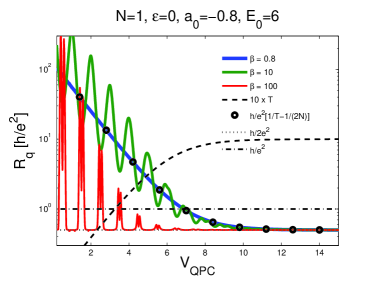
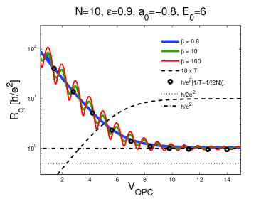
Figure 6: (Color online) $R_{q}$ as a function of $V_{QPC}$ for different temperatures for a coherent system $\varepsilon=0$ (upper panel) and for a strongly incoherent system $\varepsilon=0.9$ and $N_{\phi}=10$ (lower panel). The inverse temperature $\beta$ is given in units of the inverse level spacing $\Delta^{-1}$.

V Conclusion

In this work, we investigate the effect of decoherence on the dynamic electron transport in a mesoscopic capacitor. Extending the voltage and dephasing probe models to the AC regime, we calculate the charge relaxation resistance and the electrochemical capacitance, which together determine the RC-time of the system. Dephasing breaks the universality of the single channel, zero temperature charge relaxation resistance and introduces a dependency on the transparency of the QPC. We find that complete intra-channel relaxation alone is not sufficient to recover the two terminal resistance formula but rather yields a resistance which is the sum of the original Landauer formula and the interface resistance to the reservoir. This is also the resistance obtained in the high temperature limit of the coherent single channel system. Only in the presence of perfect inter-channel relaxation with a large number of channels, does the QD act as an additional reservoir and we recover the classically expected two terminal resistance.

Appendix A High temperature regime integrals

In this appendix we compute the integrals appearing in the high temperature limit of Eq. (29). Asymptotically we have

$$\lim_{\beta\rightarrow 0}R_{q}=\frac{h}{2e^{2}}\frac{I_{2}}{(I_{1})^{2}}\,,$$ (31)

where

$$I_{1}=\int_{0}^{\Delta}dE\nu(E),\quad\text{and}\quad I_{2}=\Delta\int_{0}^{\Delta}dE\nu(E)^{2}\,$$ (32)

with $\nu(E)=\frac{1}{\Delta}\frac{1-r^{2}}{1+2r\cos\frac{2\pi E}{\Delta}+r^{2}}$. Following a change of variables $x=\frac{2\pi E}{\Delta}$ we get

$$I_{1}=\frac{1}{2\pi}\int_{0}^{2\pi}dx\frac{1-r^{2}}{1+2r\cos x+r^{2}}\,,$$ (33)

and

$$I_{2}=\frac{1}{2\pi}\int_{0}^{2\pi}dx\frac{(1-r^{2})^{2}}{(1+2r\cos x+r^{2})^{2}}\,.$$ (34)

A simple way of computing these integrals is to use the (Poisson kernel) identity

$$\frac{1-r^{2}}{1+2r\cos x+r^{2}}=\sum_{k=-\infty}^{\infty}(-r)^{|k|}e^{ikx}\,,$$ (35)

which can easily be verified by splitting the sum as $\sum_{k=-\infty}^{\infty}x^{k}=\sum_{k=0}^{\infty}x^{k}+\sum_{k=-\infty}^{0}x^{k}-1$ and utilizing the fact that for $|r|<1$, the geometric series converge. Integrating the sum in $I_{1}$ term by term and using the identity $\int_{0}^{2\pi}e^{ikx}dx=2\pi\delta_{k0}$ for $k\in\mathbb{Z}$, we immediately find $I_{1}=1$. Similarly we have

$$I_{2} =\frac{1}{2\pi}\int_{0}^{2\pi}dx\left(\sum_{k=-\infty}^{\infty}(-r)^{|k|}e^{ikx}\right)^{2}$$

$$=\frac{1}{2\pi}\sum_{k,k^{\prime}=-\infty}^{\infty}(-r)^{|k|+|k^{\prime}|}\int_{0}^{2\pi}dxe^{i(k+k^{\prime})x}$$

$$=\sum_{k,k^{\prime}=-\infty}^{\infty}(-r)^{|k|+|k^{\prime}|}\delta_{k+k^{\prime},0}=\frac{1}{\Delta}\sum_{k=-\infty}^{\infty}(-r)^{2|k|}$$

$$=\sum_{k=0}^{\infty}(-r)^{2k}+\sum_{k=-\infty}^{0}(-r)^{-2k}-1$$

$$=\frac{2}{1-r^{2}}-1=\frac{1+r^{2}}{1-r^{2}}\,.$$ (36)

Substituting back into (31) yields the desired result.

References

- Fève et al. (2007) G. Fève, A. Mahé, J. M. Berroir, T. Kontos, B. Plaçais, D. C. Glattli, A. Cavanna, B. Etienne, and Y. Jin, Science 316, 1169 (2007).
- Moskalets et al. (2007) M. Moskalets, P. Samuelsson, and M. Büttiker, cond-mat.mes-hall/0707.1927 (unpublished) (2007).
- Kataoka et al. (2007) M. Kataoka, R. J. Schneble, A. L. Thorn, C. H. Barnes, C. J. Ford, D. Anderson, G. A. Jones, I. Farrer, D. A. Ritchie, and M. Pepper, Phys. Rev. Lett. 98, 046801 (2007).
- Blumenthal et al. (2007) M. D. Blumenthal, B. Kaestner, L. Li, S. Giblin, T. J. B. M. Janssen, M. Pepper, D. Anderson, G. Jones, and D. A. Ritchie, Nature Phys. 3, 343 (2007).
- Kaestner et al. (2007) B. Kaestner, V. Kashcheyevs, S. Amakawa, L. Li, M. D. Blumenthal, T. J. B. M. Janssen, G. Hein, K. Pierz, T. Weimann, U. Siegner, et al., cond-mat.mes-hall/0707.0993 (unpublished) (2007).
- Gabelli et al. (2006) J. Gabelli, J. M. Berroir, G. Fève, B. Plaçais, Y. Jin, B. Etienne, and D. C. Glattli, Science 313, 499 (2006).
- Büttiker et al. (1993a) M. Büttiker, H. Thomas, and A. Prêtre, Phys. Lett. A A180, 364 (1993a).
- Gopar et al. (1996) V. A. Gopar, P. A. Mello, and M. Büttiker, Phys. Rev. Lett. 77, 3005 (1996).
- Brouwer and Büttiker (1997) P. W. Brouwer and M. Büttiker, Europhys. Lett. 37, 441 (1997).
- Brouwer et al. (1997) P. W. Brouwer, K. M. Frahm, and C. W. Beenakker, Phys. Rev. Lett. 23, 4737 (1997).
- Büttiker and Nigg (2007) M. Büttiker and S. E. Nigg, Nanotechnology 18, 044029 (2007).
- Büttiker et al. (1993b) M. Büttiker, A. Prêtre, and H. Thomas, Phys. Rev. Lett. 70, 4114 (1993b).
- von Klitzing et al. (1980) K. von Klitzing, G. Dorda, and M. Pepper, Phys. Rev. Lett. 45, 494 (1980).
- Büttiker (1988a) M. Büttiker, Phys. Rev. B. 38, 9375 (1988a).
- van Wees et al. (1988) B. J. van Wees, L. P. Kouwenhoven, H. van Houten, C. W. Beenakker, J. E. Mooij, C. T. Foxon, and J. J. Harris, Phys. Rev. Lett. 60, 848 (1988).
- Wharam et al. (1988) D. A. Wharam, T. J. Thornton, R. Newbury, M. Pepper, H. Ahmed, J. E. F. Frost, D. G. Hasko, D. C. Peacock, D. A. Ritchie, and G. A. C. Jones, J. Phys. C 21, L209 (1988).
- Nigg et al. (2006) S. E. Nigg, R. López, and M. Büttiker, Phys. Rev. Lett. 97, 206804 (2006).
- Büttiker (1986) M. Büttiker, Phys. Rev. B. 33, 3020 (1986).
- Büttiker (1988b) M. Büttiker, IBM J. Res. Develop. 32, 63 (1988b).
- Datta and Lake (1991) S. Datta and R. K. Lake, Phys. Rev. B. 44, 6538 (1991).
- de Jong and Beenakker (1996) M. J. M. de Jong and C. W. J. Beenakker, Physica A 230, 219 (1996).
- Pilgram et al. (2006) S. Pilgram, P. Samuelsson, H. Förster, and M. Büttiker, Phys. Rev. Lett. 97, 066801 (2006).
- Landauer (1970) R. Landauer, Philos. Mag. 21, 863 (1970).
- Imry (1986) Y. Imry, in Directions in Condensed Matter Physics, edited by G. Grinstein and G. Mazenko (World Scientific, Singapore, 1986).
- Landauer (1987) R. Landauer, Z. Phys. 68, 217 (1987).
- Sols and Sanchez-Cañizares (1999) F. Sols and J. Sanchez-Cañizares, Superlattices and Microstructures 25, 628 (1999).
- Staring et al. (1992) A. A. M. Staring, B. W. Alphenaar, H. V. Houten, L. W. Molenkamp, O. J. A. Buyk, M. A. A. Mabesoone, and C. T. Foxon, Phys. Rev. B. 46, 12869 (1992).
- Heinzel et al. (1994) T. Heinzel, D. A. Wharam, and J. P. Kotthaus, Phys. Rev. B. 50, 15113 (1994).
- Moskalets and Büttiker (2001) M. Moskalets and M. Büttiker, Phys. Rev. B. 64, 201305 (2001).
- Chung et al. (2007) S.-W. Chung, M. Moskalets, and P. Samuelsson, Phys. Rev. B. 75, 115332 (2007).
- Clerk and Stone (2004) A. A. Clerk and A. D. Stone, Phys. Rev. B. 69, 245303 (2004).
- Polianski et al. (2005) M. L. Polianski, P. Samuelsson, and M. Büttiker, Phys. Rev. B. 72, 161302 (2005).
- Förster et al. (2007) H. Förster, P. Samuelsson, S. Pilgram, and M. Büttiker, Phys. Rev. B. 75, 035340 (2007).
- Michaelis and Beenakker (2006) B. Michaelis and C. W. J. Beenakker, Phys. Rev. B. 73, 115329 (2006).
- Prêtre et al. (1996) A. Prêtre, H. Thomas, and M. Büttiker, Phys. Rev. B. 54, 8130 (1996).
- Gabelli (2006) J. Gabelli, Ph.D. thesis, Université de Paris 6 (2006).
- Büttiker (1990) M. Büttiker, Phys. Rev. B. 41, 7906 (1990).