Are the nearby groups of galaxies gravitationally bound objects?

Abstract

We have compared numerical simulations to observations for the nearby ($<40$ Mpc) groups of galaxies (Huchra & Geller 1982 and Ramella et al. 2002). The group identification is carried out using a group-finding algorithm developed by Huchra & Geller (1982). Using cosmological N-body simulation code with the $\Lambda$CDM cosmology, we show that the dynamical properties of groups of galaxies identified from the simulation data are, in general, in a moderate, within 2$\sigma$, agreement with the observational catalogues of groups of galaxies. As simulations offer more dynamical information than observations, we used the N-body simulation data to calculate whether the nearby groups of galaxies are gravitationally bound objects by using their virial ratio. We show that in a $\Lambda$CDM cosmology about $20$ per cent of nearby groups of galaxies, identified by the same algorithm as in the case of observations, are not bound, but merely groups in a visual sense. This is quite significant, specifically because estimations of group masses in observations are often based on an assumption that groups of galaxies found by the friends-of-friends algorithm are gravitationally bound objects. Simulations with different resolutions show the same results. We also show how the fraction of gravitationally unbound groups varies when the apparent magnitude limit of the sample and the value of the cosmological constant $\Lambda$ is changed. In general, a larger value of the $\Omega_{\Lambda}$ generates slightly more unbound groups.

1 Introduction

Small groups of galaxies are the most common galaxy associations and contain $\sim 50$ per cent of all galaxies in the universe (e.g. Holmberg 1950; Humason et al. 1956; Huchra & Geller 1982; Geller & Huchra 1983; Nolthenius & White 1987). The study of galaxy groups is a very interesting area of research because these density fluctuations lie between galaxies and clusters of galaxies and may provide important clues to galaxy formation. Small groups of galaxies are also important cosmological indicators of the distribution, and properties, of dark matter in the universe.

The dynamics of the nearby groups of galaxies and the Local Group has provided a unique challenge to cosmological models in the past. The quiescence of the local peculiar velocity field (e.g. de Vaucouleurs 1958; Sandage & Tammann 1975; Sandage 1999 and Ekholm et al. 2001) was a long-standing puzzle that presented a challenge for the models of structure formation. The velocity field within 5$h^{-1}$ Mpc of the Local Group is extremely ’cold’, the dispersion is only $\sim 50-60$ km s^-1 (Teerikorpi et al. 2005 and references therein). The $\Lambda$CDM cosmology and dark energy has solved this problem and it has been shown by e.g. Klypin et al. (2003), Macció et al. (2005) and Peirani & de Freitas Pacheco (2006) with constrained simulations that the $\Lambda$CDM cosmology can produce the small values of the velocity dispersion. Today, the question of the virialization of groups of galaxies and the fraction of gravitationally bound systems provides a new challenge for the cosmological models and grouping algorithms.

Over the last two decades, cosmological simulations have proven to be an invaluable tool in testing theoretical models in the non-linear regime. The standard approach is to assume a cosmological model and to use the appropriate power spectrum of the primordial perturbations to construct a random realisation of the density field within a given simulation volume. The evolution of the initial density field is then followed by using an N-body simulation code, and the results in the simulation box (viewed from outside) are compared with observational data. A comparison of the simulations with observational data is typically done in a statistical manner. The statistical approach works well if there is a statistically representative sample of objects with well-understood selection effects for both the observed universe and the simulations.

Given a set of observed galaxies with their positions in the sky and their redshifts, the task of a group-finder is to return sets of galaxies that most likely represent true gravitationally bound structures. Some contamination is always expected due to selection effects in observations. This study uses one of the most popular group-finders: the friends-of-friends (FOF) algorithm. FOF has been used widely for identifying groups of galaxies in the redshift surveys (Huchra & Geller 1982; Geller & Huchra 1983; Nolthenius & White 1987; Ramella et al. 1989; Moore et al. 1993; Ramella et al. 1997; Ramella et al. 2002; Tucker et al. 2000 and Giuricin et al. 2000) and is now a standard approach.

The identification of the group members has, in general, been based on a subjective selection of data. In order to remove this difficulty, Huchra & Geller (1982) (hereafter HG82) developed a method of identifying groups of galaxies from the observations. It has been usually thought that the FOF based algorithms would produce groupings which are mostly gravitationally bound when the number of galaxies in a group exceeds five members (see e.g. Ramella et al. 2002). A few studies (e.g. Carlberg et al. 2001) have been made where the free parameters of the FOF algorithm have been optimised to avoid spurious groups with interlopers. Studies of the FOF algorithms have concluded that the choice of the free parameters depends on the case that is studied, and no singular best choice of the parameters can be made. Unfortunately, none of the observational methods do truly answer the question whether groups of galaxies are gravitationally bound objects. There are some estimates for the fraction of how many groups found by the FOF algorithm are spurious (see e.g. Ramella et al. 2002), but these estimates are not based on the physical properties of the groups.

Cosmological N-body simulations include all the necessary information for finding out whether a given object is gravitationally bound or not. Aceves & Velázquez (2002) studied small galaxy groups with N-body simulations and made conclusions about the virialization of the groups. Diaferio et al. (1994) studied compact groups of galaxies with N-body simulations and made remarks about the fraction of bound groups and chance alignment systems. Groups of galaxies, and their dynamical properties generated by the FOF algorithm, have been studied earlier with N-body simulations (see e.g. Nolthenius et al. 1997; Diaferio et al. 1999; Merchán & Zandivarez 2002; Casagrande & Diaferio 2006). Most of these earlier studies have taken advantage of the constrained simulations and have used models which are different from the currently popular $\Lambda$CDM cosmology. In these constrained, or mock catalogue, simulations the simulated space has been compared directly with the observations of redshift space and the groups have been categorized as spurious if the algorithm has failed to find similar groups as in real space. Instead, we have studied the virial ratio of the groups of galaxies produced by the FOF algorithm first described in HG82. We will show that $\sim 20$ per cent of the groups of galaxies found by the FOF algorithm are not real gravitationally bound groups, but spurious. Our results agree roughly with the previous results and estimates but do not confirm the claim by Ramella et al. (1989) that groups with more than four members are gravitationally bound.

For an ’observer’ placed in a specific location, selecting a similar environment between observational data and cosmological simulations might be problematic. The simplest way is to choose an ’observation’ point within a simulation box by certain criteria. It is argued (e.g. Klypin et al. 2003 and references therein) that it is not clear what ’similar environment’ actually means and that simply placing the observer at some specific point would resolve the issue. In this paper, we show that this is a useful approach, as we are not comparing simulations to observations directly but with statistics.

The main purpose of this work is to study if groups of galaxies found by the HG82 algorithm are bound, and how the fraction of bound groups depend on the chosen magnitude limit and cosmological model. We will show our findings with different apparent magnitude limits and for different cosmological models. We also show that there is no significant correlation between the crossing time of a group and its virial ratio.

This paper is organized as follows. In section 2 we review the method used in the identification of the group members in the observations. A brief discussion of the differences between observations and simulations is given in section 2. In section 3 we discuss briefly the virial ratio, used for determining whether a group of galaxies is gravitationally bound. Section 4 discusses the simulations we use for the analysis. In sections 5 and 6 we present our results and discuss the findings. Discussion of the probability functions of gravitationally unbound groups is done in section 7. Finally, we summarize our results in section 8.

2 A review of the group-finding algorithm

In observations there are generally three basic pieces of information available for the study of the galaxy distribution: the position, the magnitude and the redshift of each galaxy. Although the magnitude is important as a measure of the object’s visibility, it is usually a poor criterion for group membership. The method used for creating a group catalogue in HG82 can be summed up in two criteria: the projected separation and the velocity difference. The FOF algorithm is described in greater detail by the original authors in HG82.

The grouping method begins with a selection of an object, which has not been previously assigned to any of the existing groups. After choosing the object the next step is to search for companions with the projected separation $D_{12}$ smaller or equal to the separation $D_{L}$:

$$D_{12}=2\sin\left(\frac{\theta}{2}\right)\frac{V}{H_{0}}\lid D_{L}(V_{1},V_{2},m_{1},m_{2})~{},$$ (1)

where the mean cosmological expansion velocity is

$$V=\frac{V_{1}+V_{2}}{2}~{},$$ (2)

and the velocity difference $V_{12}$ is smaller or equal to the velocity $V_{L}$:

$$V_{12}=|V_{1}-V_{2}|\lid V_{L}(V_{1},V_{2},m_{1},m_{2})~{},$$ (3)

where $V_{1}$ and $V_{2}$ refer to the velocities (redshifts) of the galaxy and its companion, $m_{1}$ and $m_{2}$ are their magnitudes, and $\theta$ is their angular separation in the sky. If no companions are found, the galaxy is entered in a list of isolated galaxies. All companions found are added to the list of group members. The surroundings of each companion are then searched by using the same method used in the first place to find companions. This process is repeated until no further members are found.

There are a variety of prescriptions for $D_{L}$ and $V_{L}$. We adopt the method used in HG82, and assume that the luminosity function is independent of distance and position and that at larger distances only the fainter galaxies are missing. For each pair we take:

$$D_{L}=D_{0}\left(\frac{\int_{-\infty}^{M_{12}}\Phi(M)dM}{\int_{-\infty}^{M_{lim}}\Phi(M)dM}\right)^{-\frac{1}{3}}~{},$$ (4)

where the integration limits can be calculated from equations:

$$M_{lim}=m_{lim}-25-5\log(D_{F})$$ (5)

and

$$M_{12}=m_{lim}-25-5\log(V)~{},$$ (6)

and where $\Phi(M)$ is the differential galaxy luminosity function for the sample, and $D_{0}$ is the projected separation in Mpc chosen at some fiducial distance $D_{F}$. In this paper we adopt constants $D_{0}=0.63~{}\mathrm{Mpc}$ and $D_{F}=10~{}\mathrm{Mpc}$ to be same as in HG82. The effect of varying $D_{0}$ has been studied e.g. by Ramella et al. (1989) where the effects are also explained.

The limiting velocity difference is scaled in the same way as the distance $D_{L}$:

$$V_{L}=V_{0}\left(\frac{\int_{-\infty}^{M_{12}}\Phi(M)dM}{\int_{-\infty}^{M_{lim}}\Phi(M)dM}\right)^{-\frac{1}{3}}~{},$$ (7)

where the fiducial value is $V_{0}=400~{}\mathrm{km}~{}\mathrm{s}^{-1}$ and the integration limits are as above (Eq. 5 and 6). Ramella et al. (1989) varied $V_{0}$ and concluded that the results are not sensitive to the choice of $V_{0}$. This is probably related to the geometry of the large-scale structure. Frederic (1995a,b) argues that the optimal choice of $D_{0}$ and $V_{0}$ depends on the purpose for which groups are being identified. Similar claims has been made in papers where the FOF algorithm has been optimized (see e.g. Eke et al. 2004 and Berlind et al. 2006). Because of this, we also show some results when $D_{0}=0.37~{}\mathrm{Mpc}$ and $V_{0}=200~{}\mathrm{km}~{}\mathrm{s}^{-1}$ are adopted.

Note that the scaling law in Equations 4 and 7 has been questioned by many authors. Specifically, replacing the power -1/3 by -1/2 (see the argument in e.g. Nolthenius & White 1987 and Gourgoulhon et al 1992) drastically reduces the correlation between the redshift and the velocity dispersion observed in the HG82 group catalogue. However, part of this correlation is related to a selection effect rather than to the grouping algorithm, because groups with low velocity dispersion usually have few bright galaxies and so they can be seen only at low redshift. In this paper, we use the equations mentioned above for consistency with the HG82 catalogue.

For simplicity, we use the Schechter (1974) luminosity function:

$$\Phi(M)=\frac{2}{5}\Phi^{*}\ln 10\left(10^{\frac{2}{5}(M^{*}-M)}\right)^{\alpha+1}\exp^{-10^{\frac{2}{5}(M^{*}-M)}}~{},$$ (8)

where $M$ is the absolute magnitude of the object. We adopt the parameter values of $\alpha=-1.02$, $M^{*}=-19.06$, and $\Phi^{*}=0.0277$ comparable to HG82. For comparison, we use the galaxy luminosity function values of $\alpha=-1.15$, $M^{*}=-19.84$, and $\Phi^{*}=0.0172$, which were derived from the Millennium Galaxy Catalogue by Driver et al. (2007).

Our chosen values of constants and parameters needed for the FOF algorithm are exactly the same as in HG82 for consistency. We do show selected results with more recent values of constants and parameters if these results differ from the results produced with the HG82 values. Throughout this paper we adopt the parameterized Hubble constant $H_{0}=100h~{}\mathrm{km}~{}\mathrm{s}^{-1}~{}\mathrm{Mpc}^{-1}$ with $h=1.0$ for comparison with HG82 when a definite value of the Hubble constant is needed. We do not consider dust extinction in the analysis of the simulations in this paper.

3 A review of the virial theorem

In the simplest case when we have a two body system with total mass $M=m_{1}+m_{2}$ and $V$ is the relative speed of the components, the kinetic energy $T$ of the system (in the centre-of-mass coordinate system) and its gravitational potential energy $U$ (taken positive) are:

$$T=\frac{1}{2}\frac{m_{1}m_{2}}{M}V^{2}~{},$$ (9)

$$U=\frac{Gm_{1}m_{2}}{R}~{},$$ (10)

where $R$ is the size of the system and $G$ is the gravitational constant. These equations are related by a simple relation:

$$U=2T~{}.$$ (11)

However, the above relation holds only for isolated self-gravitating systems when the system is in equilibrium.

In general, groups of galaxies (and dark matter haloes) contain more than two members. Therefore a generalized method for calculating the kinetic and the potential energies is needed. We adopt a method described by Chernin & Mikkola (1991). In general, the kinetic energy may be written:

$$T=\frac{1}{2M}\sum_{i<j}m_{i}m_{j}(\mn@boldsymbol{V}_{i}-\mn@boldsymbol{V}_{j})^{2}~{},$$ (12)

and the potential energy:

$$U=G\sum_{i<j}\frac{m_{i}m_{j}}{R_{i,j}}~{},$$ (13)

where $m_{i}$ and $m_{j}$ are the masses of the two galaxies, $\mn@boldsymbol{V}_{i}$ and $\mn@boldsymbol{V}_{j}$ are their velocities, and $R_{i,j}$ is the distance between them.

We use these general equations to get the total kinetic energy of a group of haloes and compare it to its total potential energy. If the group of haloes does not fulfill the criterion:

$$T-U<0~{},$$ (14)

it is entered into a list of unbound groups. The above criterion is equal to the virial ratio:

$$\frac{T}{U}<1.0~{},$$ (15)

which we use throughout this paper as a criterion for discriminating between bound and unbound groups.

4 Description of the cosmological simulations

4.1 Background

We present results from four simulations, performed by the cosmological N-body simulation code AMIGA (Adaptive Mesh Investigations of Galaxy Assembly). The former version of AMIGA was known as MLAPM (for details see Knebe et al. 2001). For the first two runs we adopt the currently popular flat low-density cosmological model $\Lambda$CDM with $h=1.0$, $\Omega_{dm}=0.27$, $\Omega_{\Lambda}=0.73$ and $\sigma_{8}=0.83$, with two different resolutions. Both simulations were made with $256^{3}$ dark matter particles. The high resolution simulation began at the initial redshift of $z_{i}=47.96$ while the low-resolution simulation was initiated at redshift $z_{i}=38.71$. The volume employed in the high resolution simulation was $(40h^{-1}~{}\mathrm{Mpc})^{3}$ and $(80h^{-1}~{}\mathrm{Mpc})^{3}$ in the low resolution simulation corresponding to the mass resolutions of $2.86\times 10^{8}h^{-1}~{}M_{\sun}$ and $2.29\times 10^{9}h^{-1}~{}M_{\sun}$, respectively. The force resolution for the high resolution simulation is $1.8h^{-1}~{}\mathrm{kpc}$ and for the low-resolution $7.3h^{-1}~{}\mathrm{kpc}$.

For the third and the fourth simulations we adopt different cosmological models. These simulations were also performed with $256^{3}$ dark matter particles but with different values of the cosmological constant $\Lambda$. The total density of the universe was kept equal to the critical density ($\Omega=1.0$). For the third simulation we adopt $h=1.0$, $\Omega_{dm}=0.1$, $\Omega_{\Lambda}=0.9$ and $\sigma_{8}=0.83$. For the fourth simulation we adopt $h=1.0$, $\Omega_{dm}=1.0$, $\Omega_{\Lambda}=0.0$ and $\sigma_{8}=0.84$ (see Table 1).

The high resolution $\Omega_{\Lambda}=0.73$ simulation was used to understand the effects of limited resolution in N-body simulations. During this work, we found some differences between results of the high and low-resolution $\Omega_{\Lambda}=0.73$ simulations. These differences are clearly visible when the group abundances are studied (see Figures 1 $-$ 4).

Table 1: Details of the simulations analyzed in this paper.

$\Omega_{\Lambda}$	$L$	$N_{p}$	$z_{i}$	$m_{res}$	$F_{res}$	$N_{h}$
$0.73$	$40$	$256^{3}$	$47.9600$	$2.86\times 10^{8}$	$1.8$	$6700$
$0.73$	$80$	$256^{3}$	$38.7099$	$2.29\times 10^{9}$	$7.3$	$9301$
$0.90$	$80$	$256^{3}$	$31.7858$	$8.50\times 10^{8}$	$7.3$	$4937$
$0.00$	$80$	$256^{3}$	$72.8767$	$8.47\times 10^{9}$	$3.7$	$7919$

Note: $\Omega_{\Lambda}$ specifies the value of the cosmological constant, $L$ is the size of the simulation box in one dimension in $h^{-1}\mathrm{Mpc}$, $N_{p}$ is the number of dark matter particles, $z_{i}$ is the initial redshift, $m_{res}$ is the mass resolution in $h^{-1}M_{\odot}$, $F_{res}$ is the force resolution in $h^{-1}\mathrm{kpc}$, and $N_{h}$ is the total number of dark matter haloes identified from the simulation.

4.2 Halo finder and identification of the dark matter haloes

Our simulations only follow the evolution of the dark matter particles via gravitational interaction. It is expected that baryons condense and form galaxies at the centres of dark matter haloes. AMIGA N-body simulation code comes with a halo finding algorithm called MHF (MLAPM’s Halo Finder, Gill et al. 2004). For our purpose of analyzing the nearby groups of haloes we used MHF.

The general goal of a halo finder, such as MHF, is to identify gravitationally bound objects. MHF essentially uses the adaptive grids of the AMIGA to locate the haloes and the satellites of the host haloes, namely subhaloes. The advantage of reconstructing the grids to locate haloes is that they follow the density field with the exact accuracy of the simulation code and therefore no scaling length is required. For more detailed description of the MHF see Gill et al. (2004).

The minimum number of particles in a halo was set to $10$. This corresponds to a halo mass $\sim 3\times 10^{9}h^{-1}~{}M_{\odot}$ and $\sim 2\times 10^{10}h^{-1}~{}M_{\odot}$ for the high and the low-resolution simulation, respectively. A low value of the minimum number of particles in a halo ensures that even with a limited resolution, large and massive haloes are split into lighter subhaloes. For large and massive ($\sim 10^{14}h^{-1}~{}M_{\odot}$) haloes, subhaloes represent visual galaxies, masses $\sim 10^{12}h^{-1}~{}M_{\odot}$. In a typical case, the total massfraction in subhaloes is $\sim 10$ per cent, and only these are visible in our ’mock’ catalogue. In our ’mock’ catalogue, the median of individual dark matter haloes mass is $\sim 1.6\times 10^{12}h^{-1}~{}M_{\odot}$ when the $\Omega_{\Lambda}=0.73$ model and the low-resolution is adopted. The first and the third quartiles are: $\sim 7.2\times 10^{11}h^{-1}~{}M_{\odot}$ and $\sim 5.0\times 10^{12}h^{-1}~{}M_{\odot}$, respectively.

The AMIGA and its halo finder calculate automatically certain properties (e.g. position, mass, velocity etc.) of the dark matter haloes. These properties were used when the FOF algorithm was applied to generate the catalogues of groups of dark matter haloes. Subhaloes were included in our data as our purpose is to study if the groups of galaxies (dark matter haloes) are gravitationally bound objects. The results did not change substantially when the subhaloes of the more massive haloes were excluded from the analysis. This result is due to the small number of subhaloes in our low-resolution simulation. The results of the high resolution simulation show no significant difference if subhaloes were excluded because subhaloes have a relatively small mass. Due to their small masses, subhaloes are not visible at the observation point, when the apparent magnitude limit of $13.2$ is adopted.

5 Statistical properties of the nearby groups of galaxies: comparing simulations with observations

5.1 Selection of the nearby groups of haloes

A Total of ten catalogues were generated, corresponding to 10 different ’observers’, for each simulation, with different apparent magnitude limits. Ten observers are used to produce enough groups to give good statistics. Note, however, that since all ten catalogues are constructed from the same parent simulation, the scatter between statistics estimated from them might underestimate the true sampling variance.

All observation points were chosen with the following criteria:

1. observation point is $>15h^{-1}$ Mpc from the edge of the simulation box

2. a massive ($\sim 5\times 10^{14}h^{-1}~{}M_{\odot}$) Virgo -type halo is located within a distance of $\sim 20h^{-1}$ Mpc.

We did not restrict the local $<10h^{-1}$ Mpc environment of the observation points by any criteria. Although it is not clear if choosing an observation point simply by the two former criteria resolves the environment issue, we believe this to be strict enough for the statistical study of the virial ratio of groups. These criteria are justified for the statistical study, as we did not perceive a significant difference between the observation points in the low resolution simulation. Small differences between observation points were observed when the high-resolution simulation was studied, as it only includes two Virgo -type haloes. When the low-resolution simulation was studied, the location of a massive (Virgo -type) halo did not have any significant effect to our results.

The simulation data do not directly give the luminosity or the absolute magnitude of the dark matter haloes, which are needed when we are mimicking observational conditions. We use halos’ virial mass $M_{vir}$ to obtain its luminosity. To obtain the luminosity of an object in the blue band we use the relation proposed by Vale & Ostriker (2004):

$$L(M_{vir})=5.7\times 10^{9}h^{-2}L_{\odot}\frac{M_{11}^{p}}{\left[q+M_{11}^{s(p-r)}\right]^{1/s}}~{},$$ (16)

where $M_{11}$ is defined:

$$M_{11}=\frac{M_{vir}}{10^{11}h^{-1}M_{\odot}}~{}.$$ (17)

For the free parameters of the mass-luminosity function, values of $p=4.0$, $q=0.57$, $r=0.28$, and $s=0.23$ were adopted (Oguri 2006). It has been shown by Cooray & Milosavljević (2005) that the relation between the mass of a dark matter halo and its luminosity is not as straightforward as presented above. For our purposes, as the luminosity of a dark matter halo is used only to determine whether a halo is visible from the observation point, the above relation should be satisfactory. For this work we do not adopt more complex methods such as actual distributions for the mass-luminosity relation.

After the luminosity $L$ of the halo is known we obtain the apparent magnitude of the halo in the blue band from the equation:

$$m_{B}=M_{\odot_{B}}-2.5\log_{10}\left(\frac{L}{L_{\odot}}\right)+5\log_{10}\left(\frac{d}{1~{}\mathrm{Mpc}}\right)+25~{},$$ (18)

where $d$ is the distance from the observation point and the magnitude of the sun in blue band $M_{\odot_{B}}=5.47$ (Cox 2000). As seen from Equation 18, we do not include dust extinction in our study, as its effect in a statistical study like ours would be negligible.

The method described above allows us to use the apparent magnitude limit $m_{lim}=13.2$ as adopted in HG82. Group catalogues of this study are also generated with different magnitude limits in order to understand the effects of the magnitude limit in magnitude-limited samples. Unless explicitly noted, all haloes and groups referred to are from the simulations; real groups of galaxies from HG82 and UZC-SSRS2 (Ramella et al. 2002) are denoted as such.

5.2 Comparison parameters

We begin by calculating the velocity dispersion $\sigma_{v}$ of a group. In general, the velocity dispersion of a group is defined as:

$$\sigma_{v}=\sqrt{\frac{1}{N_{H}-1}\sum_{i=1}^{N_{H}}(v_{i}-<v_{R}>)^{2}}~{},$$ (19)

where $N_{H}$ is the number of haloes (or galaxies) in a group, $v_{i}$ is the radial velocity of the $i$th halo (or galaxy) and $<v_{R}>$ is the mean group radial velocity.

The second comparison parameter is the mean pairwise separation $R_{p}$ which is a measure of the size of a group. It can be defined as:

$$R_{p}=\frac{8<v_{R}>}{\pi H_{0}}\sin\left(\frac{1}{N_{H}(N_{H}-1)}\sum_{j<i}^{N_{H}}\sum_{i=1}^{N_{H}}\theta_{ij}\right)~{},$$ (20)

where $<v_{R}>$ is the mean group radial velocity, $H_{0}$ is the Hubble constant, and $\theta_{ij}$ is the angular separation of the $i$th and $j$th group members. Other two comparison parameters are the total group mass and the virial crossing time (in units of the Hubble time $H_{0}^{-1}$) which can be defined as:

$$t_{c}=\frac{3R_{H}}{5^{3/2}\sigma_{v}}~{},$$ (21)

where $\sigma_{v}$ is the velocity dispersion and $R_{H}$ is the mean harmonic radius:

$$R_{H}=\frac{\pi<v_{R}>}{H_{0}}\sin\left\{\frac{1}{2}\left[\frac{N_{H}(N_{H}-1)}{2}\left(\sum_{i=1}^{N_{H}}\sum_{j>i}^{N_{H}}\theta_{ij}\right)^{-1}\right]\right\}$$ (22)

where all the variables are defined as above.

In observations, the group masses can be estimated in various methods. In the HG82 and the UZC-SSRS2 catalogues the total mass of a group is estimated with a simple relation:

$$M_{obs}=6.96\times 10^{8}\sigma_{v}^{2}R_{H}M_{\odot}~{},$$ (23)

where $\sigma_{v}$ is the velocity dispersion, and $R_{H}$ is the mean harmonic radius of the group as defined above. We use this simple relation to determine the ’observable’ mass of a group when we are comparing the masses of the simulated groups to the real observed groups such as HG82 and UZC-SSRS2. However, when the total mass of a group is used to scale the properties of groups (in Section 6), we calculate the total mass of a group of dark matter haloes as a sum of the member halo masses, namely the ’true’ mass of the group. In case of the subhaloes, the diffuse dark matter is included in the main halo’s mass. In general, we do not include the diffuse dark matter within a given distance from the group centre, as it would be troublesome to choose an appropriate distance. We do not consider this error to be meaningful, as the diffuse dark matter does not substantially give rise to the mean density of a simulation.

5.3 Comparison with observations

Comparison between simulations and observations are done using a Kolmogorov-Smirnov (K-S) test. The null hypothesis $H_{null}$ of the K-S test is that the two distributions are alike and are drawn from the same population distribution function. Results of the K-S tests are presented as significance levels (value of the $Q$ function) for the null hypothesis. Correlation between two variables is proved or disproved with the use of the linear correlation coefficient $r$. In general, the significance level of $0.001$ is adopted when the correlation between two variables is determined. For correlations we also present a probability $P(r)$ of observing a value of the correlation coefficient greater than $r$ for a sample of $N$ observations with $N-2$ degrees of freedom.

We begin the comparison of our simulations to observations by using the parameters presented in the previous subsection. A direct comparison between HG82 and simulations is possible as the magnitude limit ($13.2$) and the depth of the catalogues ($cz<4,000$ km s^-1) are comparable. Comparisons with the more recent group catalogue UZC-SSRS2 is also done. The UZC-SSRS2 catalogue has the magnitude limit of $15.5$ and only galaxies with $cz<15,000$ km s^-1 has been considered. These differences make the direct comparison of the UZC-SSRS2 with the simulations less conclusive. We also compare our ten observation points with each other but do not find significant difference between them. This justifies our method of choosing the observational points as stated before.

In Figures 1 $-$ 5 the abundance of groups is scaled to the volume of a sample as the distributions depend strongly on selection and volume effects. However, as there is no ’total’ volume of a galaxy sample in magnitude-limited group catalogues, we weight each group according to its distance (Moore et al. 1993 and Diaferio et al. 1999). As we only consider groups with three or more members, we can identify a group only when its third-brightest galaxy has an absolute magnitude

$$M_{i}\leq m_{lim}-25-5\log(\frac{<cz>}{H_{0}})~{},$$ (24)

where $<cz>$ is the mean velocity of the group. $M_{i}$ determines the radius $cz_{i}$ of a sphere within which we could have identified this group.

We calculate the comoving volume sampled by a group with the following equation:

$$\Psi_{i}=\frac{\omega}{3}\left(\frac{cz_{i}}{H_{0}}\right)^{3}\left[1-\frac{3z_{i}}{2}\left(1+\frac{\Omega}{2}\right)\right]~{},$$ (25)

where $\omega$ is the solid angle of the catalogue, $z_{i}$ is the redshift of the group, $c$ is the speed of light, and $\Omega$ is the cosmological density parameter, taken as $1.0$. Each group of galaxies (or dark matter haloes) contributes with a weight of $\Psi_{i}^{-1}$ to the total abundance of groups. We include all galaxies with $cz>500$ km s^-1. This lower cut-off avoids including faint objects that are close to the observation point as these groups could contain galaxies fainter than real magnitude-limited surveys. Therefore we consider only groups with $<cz>$ larger than $500$ km s^-1 in mock, HG82, and UZC-SSRS2 catalogues.

Figures 1 $-$ 4 show that the $\Lambda$CDM simulations are, in general, in a moderate agreement with observations when the resolution effects of the N-body simulations are taken into account. Our $\Lambda$CDM simulations are within 2$\sigma$ from the UZC-SSRS2 catalogue and within 3$\sigma$ from the HG82 catalogue. Figures 1 $-$ 4 are all from the $\Omega_{\Lambda}=0.73$ simulations when the apparent magnitude limit has been set to $13.2$, comparable to HG82. The error bars in Figures 1 $-$ 4 are the standard deviation between ten observation points. Unless explicitly noted, the simulations referred to are $\Omega_{\Lambda}=0.73$ simulations, other models are denoted as such.

5.3.1 Velocity dispersion

Figure 1 shows that the cosmological $\Omega_{\Lambda}=0.73$ model can produce velocity dispersions similar to observations (see also Klypin et al. 2003, Macció et al. 2005 and Peirani & de Freitas Pacheco 2006). Figure 1 agrees with results by Casagrande & Diaferio (2006) (their Figure 14) even though Casagrande & Diaferio (2006) considered only groups with $>5$ members. Our low-resolution simulation produces roughly the right number density of groups when the high ($>100$ km s^-1) velocity dispersions are considered and the comparison is carried out against more recent observations (UZC-SSRS2). However, due to the limited mass resolution, the low-resolution simulation lacks a significant number of groups when the abundance of groups with velocity dispersions $<100$ km s^-1 is studied. Because of this discrepancy the applied K-S test fails: $Q\sim 10^{-6}$ (against the HG82) and $Q\sim 10^{-6}$ (against the UZC-SSRS2). Even-though the K-S test fails, the low-resolution simulation is within 3$\sigma$ from the HG82. When the high-resolution simulation is considered we get roughly the same number density of groups as in observations. However, the high resolution simulation lacks groups with velocity dispersions $>500$ km s^-1. This can be explained by the small volume of the high-resolution simulation. Even with this discrepancy, the applied K-S tests are approved with the significance levels of $0.02$. When observations (HG82 and UZC-SSRS2) are compared against each other, the applied K-S test is approved at level of $0.34$. For detailed significance levels of the K-S tests see Table 3.

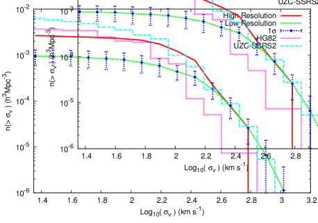
Figure 1: The cumulative number density of velocity dispersion $\sigma_{v}$ for galaxy groups. Simulation data are from the $\Omega_{\Lambda}=0.73$ simulations, and it is averaged over the ensemble of ten mock catalogues. The error bars are 1$\sigma$ errors and are only shown for the low-resolution $\Omega_{\Lambda}=0.73$ simulation for clarity. The error bars for other data have similar size.

5.3.2 Mass

Figure 2 shows that the cosmological $\Lambda$CDM model can produce ’observable’ masses (Eq. 23) similar to observations when the resolution effects of the simulations are considered. The low-resolution simulation can produce the same number density of groups as in the UZC-SSRS2 catalogue when massive ($\log$(Group Mass M${}_{\odot}^{-1})>13.5$) groups are considered. Both the UZC-SSRS2 catalogue and the low-resolution mock catalogue has an excess of massive groups if comparison is carried out against the HG82 catalogue. When less massive groups ($\log$(Group Mass M${}_{\odot}^{-1})<13.0$) are studied, the low-resolution simulation has a number density of groups which is over 3$\sigma$ lower than in the UZC-SSRS2 catalogue. The resolution effect is clearly visible in Figure 2 when the high resolution simulation is studied, as it can produce about the right number density of groups when less massive ($\log$(Group Mass M${}_{\odot}^{-1})<13.0$) groups are considered. The high-resolution simulation is less than 1$\sigma$ away from the HG82 and within 2$\sigma$ from the UZC-SSRS2 even when groups with $\log$(Group Mass M${}_{\odot}^{-1})<11.0$ are considered. The applied K-S test is approved ($Q\sim 0.58$) only when the high-resolution simulation is compared to the HG82 catalogue. In all other cases the K-S test fails. For numerical details of the K-S test, see Table 3.

As the ’observable’ mass of a group depends strongly on the groups’ velocity dispersion (see Equation 23) we made another comparison between group abundances by mass. If we use the ’true’ mass of a group instead of an ’observable’ mass, other differences arise. There is no substantial difference between the plots of ’observable’ and ’true’ mass when comparing the abundances of lighter ($\log$(Group Mass M${}_{\odot}^{-1})<14.0$) groups. However, our simulations do not produce a single group with a ’true’ mass $>5\times 10^{14}h^{-1}$M_⊙. The low and high-resolution $\Omega_{\Lambda}=0.73$ simulations show the same cut-off, thus the lack of massive groups is not a resolution effect. However, the small volume of our simulation boxes explains the lack of massive groups in simulations and the existence of groups with large ’observed’ mass is due to projection effects, which are not realiably taken into account in Eq. 23.

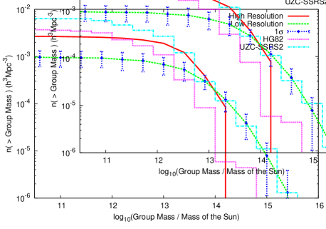
Figure 2: Group abundance by ’observable’ mass of the groups. Simulation data are from the $\Omega_{\Lambda}=0.73$ simulations, and it is averaged over the ensemble of ten mock catalogues. The error bars are 1$\sigma$ errors and are only shown for the low-resolution $\Omega_{\Lambda}=0.73$ simulation for clarity. The error bars for other data have similar size.

5.3.3 Size

The cosmological $\Omega_{\Lambda}=0.73$ model can produce groups of haloes which are similar in size to observed groups. Note, however, that we do not compare our simulations to the UZC-SSRS2 catalogue, as it doesn’t contain the information about the pairwise separtion of groups. Our high-resolution simulation produces about the right number density of groups when small ($\log$(R_p) $<-0.4$) groups are considered and the error is well within 1$\sigma$. The high-resolution simulation seems to produce an excess of groups when intermediate size ($\log$(R_p) $\in[-0.3,0.4]$) groups are considered. However, as the only comparison observation is the HG82 catalogue this excess might not be as large as in Figure 3, as other comparisons (Figures 1 and 2) show that the HG82 and the UZC-SSRS2 catalogues differ quite significantly from each other.

When the low-resolution simulation is studied, we observe this same excess when larger ($\log$(R_p) $>0.1$) groups are considered. Because of these discrepancies the applied K-S test fails in both cases, with $Q\sim 10^{-3}$ and $Q\sim 10^{-5}$ for the high and the low-resolution simulations, respectively. Even though the K-S test fails, the simulated mock catalogues of group abundances by mean pairwise separation are mostly within 2$\sigma$.

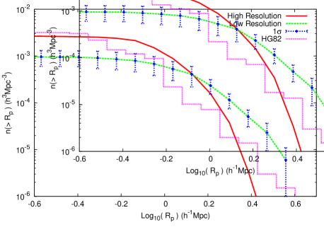
Figure 3: The cumulative distribution of mean pairwise separation $R_{p}$ for galaxy groups. Simulation data are from the $\Omega_{\Lambda}=0.73$ simulations, and it is averaged over the ensemble of ten mock catalogues. The error bars are 1$\sigma$ errors and are only shown for the low-resolution $\Omega_{\Lambda}=0.73$ simulation for clarity. The error bars for other data have similar size.

5.3.4 Crossing time

Figure 4 shows that the cosmological $\Omega_{\Lambda}=0.73$ model can produce groups with crossing times similar to the HG82 observations. The low-resolution simulation produces the number density of groups with small crossing times, which is a lot lower than observed. However, this discrepancy is due to limited resolution, as the high-resolution simulation produces a lot more groups with small crossing times. The high-resolution simulation produces roughly the right number density of groups when the crossing time of the group is studied. Some differences are observed when larger ($\log$(t_c) $>-0.6$) crossing times are studied. Both simulations produce a higher number density than observed. For low-resolution simulation this excess is not large as the number density is within 2$\sigma$. Because of the discrepancies visible in Figure 4, the applied K-S test fails in both cases. For numerical details, see Table 3. When more recent values of the Schechter luminosity function are adopted, somewhat lower crossing times are observed in general. However, more recent values of the Schechter luminosity function do not give a better agreement, and the K-S test fails. The significance levels of the K-S tests are $\sim 10^{-4}$ and $\sim 10^{-5}$, respectively.

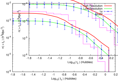
Figure 4: The cumulative distribution of crossing time $t_{c}$ (in unit of the Hubble time) for galaxy groups. Simulation data are from the $\Omega_{\Lambda}=0.73$ simulations, and it is averaged over the ensemble of ten mock catalogues. The error bars are 1$\sigma$ errors and are only shown for the low-resolution $\Omega_{\Lambda}=0.73$ simulation for clarity. The error bars for other data have similar size.

Our simulations with the FOF algorithm do not (with a few exceptions) contain groups with crossing time larger than one Hubble time. For the high-resolution simulation, the median value of the crossing time is $0.14H_{0}^{-1}$. The median value of the crossing time for the HG82 catalogue and for the low-resolution simulation is $0.19H_{0}^{-1}$. Small crossing times suggests that groups of galaxies have had time to virialize and these groups should be gravitationally bound (see e.g. Gott & Turner 1977; Tucker et al. 2000; Aceves & Velázquez 2002 and Plionis et al. 2006). We studied the correlation between crossing time and virial ratio and did not find any significant relation between these two variables. The linear correlation coefficient of $-0.01$ suggests that there is no correlation between crossing time and virial ratio, in the low-resolution simulation when the apparent magnitude limit of $13.2$ is adopted. This correlation is not significant at level of $0.05$ and $P(r)\sim 0.29$. There is no significant correlation between these two variables when different values of $\Omega_{\Lambda}$, resolutions or the apparent magnitude limits are adopted (see Table 2). The lack of correlation between virial ratio and crossing time (see similar results in Diaferio et al. 1993) calls into question the crossing time as an estimator of gravitationally bound systems which is widely accepted in observations.

Table 2: The correlation between crossing time and virial ratio when different values of $\Omega_{\Lambda}$ and the apparent magnitude limits are adopted.

$\Omega_{\Lambda}$	$m_{lim}$	$r$	$\alpha$	$P(r)$
$0.00$	$13.2$	$-0.009$	$>0.05$	$0.33$
$0.00$	$20.0$	$0.005$	$>0.05$	$0.36$
$0.73^{H}$	$13.2$	$-0.016$	$>0.05$	$0.26$
$0.73^{L}$	$13.2$	$-0.016$	$>0.05$	$0.29$
$0.73^{L}$	$20.0$	$-0.016$	$>0.05$	$0.09$
$0.90$	$13.2$	$-0.012$	$>0.05$	$0.42$
$0.90$	$20.0$	$-0.022$	$>0.05$	$0.09$

Note: $\Omega_{\Lambda}$ specifies the value of the cosmological constant (^H = high-resolution and ^L = low-resolution simulation), $m_{lim}$ is the apparent magnitude limit of the search, $r$ is the value of the linear correlation coefficient, $\alpha$ is the significance level, and $P(r)$ is the probability of observing a value of the correlation coefficient greater than $r$.

5.3.5 Richness

The $\Omega_{\Lambda}=0.73$ model can produce groups comparable to observations when the number of members in a group is studied. The abundance of ’rich’ groups is roughly the same in the low-resolution simulation as in the observations. However, the low-resolution simulation cannot produce as many ’poor’ groups as is observed. The lack of ’poor’ ($<4$) and the excess of ’intermediate’ ($\in[6,40]$) groups is the reason why the K-S test fails ($Q\sim 10^{-5}$). The agreement is even worse ($Q\sim 10^{-7}$) when more recent values of Schechter luminosity function are adopted. These values ($\alpha=-1.15$, $M^{*}=-19.84$, and $\Phi^{*}=0.0172$) produce a large number of ’poor’ groups and a lack of ’rich’ groups. The difference between the low-resolution simulation and observations is due to the limited resolution in the simulations. When the high-resolution simulation is used, the agreement to observations, especially to UZC-SSRS2, is better ($Q\sim 10^{-3}$).

5.3.6 Influence of dark energy

There are big differences between different cosmological models when dynamical properties of groups of dark matter haloes are studied. Figure 5 shows the impact of dark energy on the formation of galaxy groups. It is clear that the $\Omega_{\Lambda}=0.0$ simulation over produces groups with high velocity dispersions. The excess is over 3$\sigma$ if the comparison is carried out to the HG82 catalogue. A smaller discrepancy is observed when the comparison is carried out to the UZC-SSRS2 catalogue. The small number density of small velocity dispersion groups can be explained by the resolution effect which is also visible in Figure 1. Because of these discrepancies the K-S tests fails. When the $\Omega_{\Lambda}=0.90$ simulation is studied, a qualitatively better agreement is observed, especially when the comparison is carried out to the HG82 catalogue. The great difference in the number density of small velocity dispersion groups can be explained by the resolution effect and the fact that the $\Omega_{\Lambda}=0.90$ simulation has relatively small number of groups. Because of the great discrepancy in the number density of small velocity dispersion groups, the applied K-S test fails in both cases.

The $\Omega_{\Lambda}=0.0$ cosmology produces more massive groups with greater velocity dispersion than the $\Lambda$CDM cosmology. Larger number of massive groups can partially be explained by the somewhat lower mass resolution in the $\Omega_{\Lambda}=0.0$ simulation. However, the excess of massive groups is most likely due to Equation 23, which we use to obtain the ’observable’ mass of a group, which depends strongly on the velocity dispersion of the group. For numerical details of K-S tests, see Table 3.

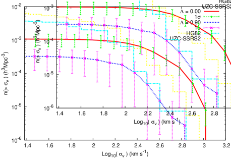
Figure 5: The cumulative distribution of velocity dispersion $\sigma_{v}$ for galaxy groups from two different simulations with two different values of the cosmological constant $\Omega_{\Lambda}$ when the apparent magnitude limit of $13.2$ has been adopted. The simulation data are averaged over the ensemble of ten mock catalogues. For comparison also the observational data from the HG82 and the UZC-SSRS2 catalogue have been plotted. The standard $\Omega_{\Lambda}=0.73$ simulations are shown in Figure 1.

Table 3: Comparison of HG82, UZC-SSRS2, and simulations when the apparent magnitude limit of $13.2$ is adopted.

$\Omega_{\Lambda}$		HG82	UZC-SSRS2	HG82 vs. UZC-SSRS2
$0.00$	$\sigma_{v}$	$10^{-5}$	$10^{-6}$	$0.34$
$0.73^{H}$	$\sigma_{v}$	$0.02$	$0.02$	$0.34$
$0.73^{L}$	$\sigma_{v}$	$10^{-6}$	$10^{-6}$	$0.34$
$0.90$	$\sigma_{v}$	$10^{-6}$	$10^{-7}$	$0.01$
$0.00$	$M_{G}$	$10^{-5}$	$10^{-6}$	$10^{-3}$
$0.73^{H}$	$M_{G}$	$0.58$	$10^{-5}$	$10^{-3}$
$0.73^{L}$	$M_{G}$	$10^{-6}$	$10^{-6}$	$10^{-3}$
$0.90$	$M_{G}$	$10^{-6}$	$10^{-7}$	$10^{-3}$
$0.73^{H}$	$R_{p}$	$10^{-3}$	$-$	$-$
$0.73^{L}$	$R_{p}$	$10^{-5}$	$-$	$-$
$0.73^{H}$	$t_{c}$	$10^{-4}$	$-$	$-$
$0.73^{L}$	$t_{c}$	$10^{-5}$	$-$	$-$

Note: Significance levels of the K-S test for the null hypothesis that observations and the simulations (^H = high-resolution and ^L = low resolution) are alike and are drawn from the same parent population (HG82 and UZC-SSRS2 columns). Significance levels of the K-S test for the null hypothesis that the HG82 and the UZC-SSRS2 group catalogue are alike and are drawn from the same parent population (HG82 vs. UZC-SSRS2 column).

5.3.7 Median values and other properties

The median values of the group properties are presented in Table 4. In general, our simulations seem to produce groups which median value of the velocity dispersion and the group mass is greater than in observations. In simulations, groups have also a greater median value for the mean pairwise separation than in the HG82 sample. The $\Omega_{\Lambda}=0.73$ simulations have the median value of velocity dispersions which are close to observations, even though they are somewhat higher. In general, median values of the group properties are in a moderate agreement with the results of similar studies (e.g. Casagrande & Diaferio 2006 and Diaferio et al. 1999). Casagrande & Diaferio (2006) found larger values for the median velocity dispersions and group masses, but they considered only groups with $>5$ members, which most likely makes the median values of groups somewhat higher.

Table 4: Weighted quartiles of the group properties.

	$\Omega_{\Lambda}=0.00$	$\Omega_{\Lambda}=0.73^{H}$	$\Omega_{\Lambda}=0.73^{L}$	$\Omega_{\Lambda}=0.90$	HG82	UZC-SSRS2
$\sigma_{v}$	$178/307/403$	$135/180/295$	$103/160/298$	$124/209/271$	$60/135/155$	$60/130/178$
$\log M_{G}$	$13.6/14.0/14.4$	$12.7/13.2/13.5$	$12.8/13.6/14.0$	$12.7/13.1/13.5$	$12.0/12.4/13.2$	$12.1/12.8/13.3$
$R_{p}$	$0.85/1.38/1.57$	$0.81/1.21/1.47$	$0.80/0.99/1.24$	$0.72/1.01/1.20$	$0.44/0.54/1.00$	$-$
$t_{c}$	$0.09/0.14/0.25$	$0.07/0.14/0.19$	$0.10/0.19/0.27$	$0.09/0.17/0.23$	$0.10/0.19/0.27$	$-$

Note: Quantities $\sigma_{v}$, $\log M_{G}$, $R_{p}$, and $t_{c}$ are in units of km s^-1, h^-1M_⊙, h^-1 Mpc, and Hubbles, respectively.

The fractions of isolated galaxies, binary galaxies and groups of galaxies were also studied. If we compare our results with HG82, a significant difference in the fraction of isolated galaxies is noticed. Comparison to the LEDA (Giudice 1999) catalogue shows a better fit. For more details, see Table 5. Tucker et al. (2000) listed a large fraction of galaxies in groups from different group catalogues. These results and comparisons are not shown in this paper due to the different magnitude limits and grouping algorithms adopted in those observations. We may state that, in general, simulations show similar results to observations (excluding HG82), with regard to the fractions of groups, binaries and isolated galaxies.

Table 5: Fractions of isolated galaxies, binary galaxies, and groups.

Source	$m_{lim}$	Groups ($\%$)	Binaries ($\%$)	Isolated ($\%$)
Simu	$13.2$	$38.1\pm 0.5$	$19.7\pm 0.1$	$42.2\pm 0.5$
Simu	$20.0$	$41.2\pm 0.2$	$17.6\pm 0.1$	$41.2\pm 0.2$
HG82	$13.2$	$60.0$	$14.0$	$26.0$
LEDA	$14.0$	$33.3\pm 0.5$	$17.1\pm 0.3$	$49.6\pm 0.4$

Note: Source refers to the sample (Simu $=$ the low-resolution $\Omega_{\Lambda}=0.73$ simulation), $m_{lim}$ is the apparent magnitude limit (in $m_{B(0)}$ except for LEDA in $B_{T}^{0}$), Groups ($\%$) is the fraction of galaxies in the groups, Binaries ($\%$) is the fraction of galaxies forming double systems, and Isolated ($\%$) is the fraction of galaxies which are not classified into any group or double system. Poisson error limits have been calculated for the samples.

We also made an attempt to study discordant redshifts in compact groups observed e.g. by Sulentic (1984) and Girardi et al. (1992). This effect has been studied by several authors (see e.g. Byrd & Valtonen 1985, Valtonen & Byrd 1986 and Iovino & Hickson 1997) who have come up with different explanations. According to these authors, apparent discordant redshifts arise when groups are not virialized and their central galaxies are incorrectly identified. Our findings are not conclusive as we did not have any exact method to identify which dark matter haloes might represent observable spiral galaxies. We did not observe any significant asymmetry in the radial velocities of the groups and neither this asymmetry was seen in the groups, which were misidentified (so that the brightest member is not the dominant member). No significant difference for the radial velocity asymmetry was discovered between bound and unbound groups.

6 Gravitationally bound groups

Gravitationally bound groups are determined by using the criterion (virial ratio, Eq. 15) presented in Section 3. This method of computing the gravitational potential well of a group does assume that the group is isolated. This is not strictly true as each group is embedded in the large-scale matter distribution, which might have an effect to the threshold $1.0$ of the virial ration $T/U$. However, we believe this effect to be negligible in a statistical study like ours.

Our study shows that $\sim 20$ per cent of groups generated by the FOF algorithm are not gravitationally bound when the $\Omega_{\Lambda}=0.73$ model is adopted. This result is in agreement with Diaferio et al. (1994), who derived a similar result for the compact groups of galaxies. If we vary the apparent magnitude limit of the search from the original $13.2$ to $20.0$, even more groups ($\sim 37$ per cent) are unbound. This is not a negligible fraction considering that one widely accepted and applied method of calculating a group mass, from observations, is based on the assumption that groups found by the FOF algorithm are, in general, gravitationally bound systems.

If we vary the value of the cosmological constant from the original $0.73$ to $0.90$, a slightly larger fraction of groups seems to be unbound when the apparent magnitude limit of $13.2$ is adopted. This result is intuitively reasonable. If the negative vacuum pressure of space is larger, gravitational force becomes ’weaker’ and a smaller number of dark matter haloes are formed and fewer groups are gravitationally bound objects. How does the fraction of gravitationally unbound groups change when the negative vacuum pressure of space is lowered? If the value of the cosmological constant is put to $0.0$, about the same fraction of groups (with $m_{lim}=13.2$) are spurious as in the $\Omega_{\Lambda}=0.90$ cosmology. When the apparent magnitude limit is changed to $20.0$, $\sim 37$ per cent of the groups are spurious (for details, see Table 6).

Table 6: Fractions of gravitationally bound groups of dark matter haloes when different cosmological models and apparent magnitude limits have been adopted.

$\Omega_{\Lambda}$	$m_{lim}$	$N_{groups}$	$f_{bound}$ ($\%$)	$N_{isolated}$ ($\%$)
$0.00$	$13.2$	$2675$	$79.2$	$20.9$
$0.00$	$20.0$	$6213$	$64.5$	$41.8$
$0.73^{H}$	$13.2$	$1570$	$70.1$	$32.8$
$0.73^{L}$	$13.2$	$1168$	$81.1$	$42.2$
$0.73^{L}$	$20.0$	$6807$	$62.7$	$41.2$
$0.90$	$13.2$	$238$	$77.3$	$53.1$
$0.90$	$20.0$	$3678$	$62.0$	$36.5$

Note: $\Omega$_Λ specifies the value of the cosmological constant (^H = high-resolution and ^L = low-resolution simulation), $m_{lim}$ is the apparent magnitude limit of the search, $N_{groups}$ is the number of groups found from ten observation points, $f_{bound}$ is the fraction of gravitationally bound groups, and $N_{isolated}$ is the percentage of the isolated haloes which do not belong to any group or binary system.

In the low-resolution $\Omega_{\Lambda}=0.73$ simulation the fraction of gravitationally bound groups rises from $81.1$ to $81.7$ per cent, when more recent values of the Schechter luminosity function are adopted. Meanwhile the total number of groups decreases $\sim 10.0$ per cent. The fraction of gravitationally bound groups rises from $81.1$ to $82.8$ per cent, when the values of the free parameters of $D_{0}=0.37~{}\mathrm{Mpc}$ and $V_{0}=200~{}\mathrm{km}~{}\mathrm{s}^{-1}$ are adopted. This result agrees with Frederic (1995a,b) who obtained similar result while studying group accuracy as a function of $D_{0}$ and $V_{0}$. Frederic (1995a,b) showed that smaller values of $D_{0}$ and $V_{0}$ produces groups with greater accuracy and these groups should be gravitationally bound.

Adopting the values of $D_{0}=0.37~{}\mathrm{Mpc}$ and $V_{0}=200~{}\mathrm{km}~{}\mathrm{s}^{-1}$ have a significant effect to the total number of groups found from the simulations. The low-resolution $\Omega_{\Lambda}=0.73$ simulation produces, in all, $1168$ groups of dark matter haloes when the original values ($D_{0}=0.63~{}\mathrm{Mpc}$ and $V_{0}=400~{}\mathrm{km}~{}\mathrm{s}^{-1}$) of the free parameters are adopted. When $D_{0}=0.37~{}\mathrm{Mpc}$ and $V_{0}=200~{}\mathrm{km}~{}\mathrm{s}^{-1}$ are adopted, the total number of groups found from the low-resolution simulation drops to $661$ while the fraction of isolated haloes rises from $\sim 42.2$ to $\sim 64.9$ per cent. Also, the group abundances changes significantly as the richest group found from the low-resolution simulation with $D_{0}=0.37~{}\mathrm{Mpc}$ and $V_{0}=200~{}\mathrm{km}~{}\mathrm{s}^{-1}$ has only $15$ members. These results are due to the fact that the limiting density enhancement of the search is inversely proportional to $D_{0}^{3}$.

Our study shows that the $\Omega_{\Lambda}=0.0$ model produces about the same fraction of bound groups as the $\Omega_{\Lambda}=0.90$ model when the apparent magnitude limit is $13.2$. However, the $\Omega_{\Lambda}=0.73$ model produces more gravitationally bound systems than the two other models we study when the original apparent magnitude limit is adopted. If the apparent magnitude limit is changed to $20.0$, the $\Omega_{\Lambda}=0.0$ model produces a slightly larger fraction of gravitationally bound groups than the $\Omega_{\Lambda}=0.73$ or the $\Omega_{\Lambda}=0.90$ simulations (for details see Table 6). The use of the apparent magnitude limit of $20.0$ means simply that every single dark matter halo in a simulation box is visible at the observation point. This result is not without bias as the simulation box is of finite size and the edge effects might become significant, even using the periodic boundary conditions in the simulations.

The calculation that determines whether a group is bound is based on three parameters: the total mass of the group, the relative velocity of the group members and the physical size of the group. In the following we will study how sensitive the result is on the values of these parameters. But first we will study the virial ratio as a function of the number of members in the group. Figure 6 shows the virial ratio $T/U$ as a function of the number of haloes in the group, namely richness. The data come from the low-resolution $\Omega_{\Lambda}=0.73$ simulation with $m_{lim}=13.2$. There are, in all, $1168$ groups of haloes seen from ten different observation points. The fractions of bound ’poor’ and ’rich’ groups are shown in Table 7.

From Figure 6 we see that groups with more than 10 members are most likely gravitationally bound and groups with three to five members are quite often unbound. Ramella et al. (1997) argues that among groups with three members, $50$ to $75$ per cent of groups are spurious. They also conclude that for groups with more than three members the fraction of spurious groups is less than $30$ per cent and may be as small as $10$ per cent. Our findings are similar, and the fraction of bound groups with four or more members is about as high as Ramella et al. (1997) suggested. Ramella et al. (2002) find that for groups with five or more members at least $80$ per cent of the groups are probably physical systems, but that $40$ to $80$ per cent of the groups with five or more members are bound groups. Our findings confirm the latter result. However, these results cannot be directly compared with ours, as slightly different values of the free parameters are adopted for the FOF algorithm. Even-though the free parameters of the FOF seem to have only a small effect to the fraction of spurious groups in our study.

Our findings for the $\Omega_{\Lambda}=0.73$ cosmology are similar to Ramella et al. (1997) for ’poor’ (three or four members) groups, as can be seen in Figure 6 and Table 7. However, our findings do not confirm the claim by Ramella et al. (1997) that among groups with three members, $50$ to $75$ per cent of groups are spurious as we find only $\sim 23$ per cent of groups with three members to be gravitationally unbound with $m_{lim}=13.2$. For the apparent magnitude-limited sample ($m_{lim}=13.2$ comparable to HG82), we found $\sim 21$ per cent of the groups with three or four haloes to be spurious. ’Rich’ groups with five or more members are more often gravitationally bound than ’poor’ groups, but the difference is relatively small at the apparent magnitude limit of $13.2$ as for ’rich’ groups, we found $\sim 15$ per cent of the groups to be spurious. This is close to the upper limit proposed by Ramella et al. (1997, 2002). More details of our findings with different abundances and apparent magnitude limits are listed in Table 7.

Table 7: Fractions of gravitationally bound ’poor’ and ’rich’ groups of dark matter haloes generated from the low-resolution $\Omega_{\Lambda}=0.73$ simulation.

$m_{lim}$	$N_{haloes}$	$N_{groups}$	$f_{bound}$ ($\%$)
$13.2$	$3$	$448$	$77.0$
$13.2$	$\in[3,4]$	$697$	$78.5$
$13.2$	$>4$	$471$	$84.9$
$20.0$	$3$	$2786$	$55.6$
$20.0$	$\in[3,4]$	$4147$	$56.3$
$20.0$	$>4$	$2660$	$72.6$

Note: $m$_lim is the apparent magnitude limit of a sample, $N_{haloes}$ is the number of haloes in a group, $N_{groups}$ is the number of groups found from ten observation points with appropriate number of haloes, and $f_{bound}$ is the fraction of gravitationally bound groups.

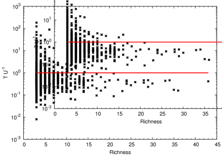
Figure 6: Virial ratio ($TU^{-1}$) versus the number of members in a group (Richness). Groups with more than 10 members are more often bound than ’poor’ groups with three to five members. The data are from the low-resolution $\Omega_{\Lambda}=0.73$ simulation when the apparent magnitude limit of $13.2$ has been adopted.

In Figure 7, the virial ratio is plotted as a function of the velocity dispersion $\sigma_{v}$ of the group. The plot shows a weak correlation in the sense that groups with large velocity dispersion are more often gravitationally unbound than groups with small velocity dispersion. The linear correlation coefficient of $0.17$ suggests that the correlation in Figure 7 is weak. However, the correlation is significant at level of $0.001$ and $P(r)\sim 10^{-8}$. The rms line plotted in Figures 7 $-$ 11 is of the form $\frac{T}{U}\propto\sigma_{v}^{b}$ or $\frac{T}{U}\propto N(haloes)^{b}$. The value of the parameter $b$ of the rms line in Figure 7 is $b=0.10\pm 0.04$.

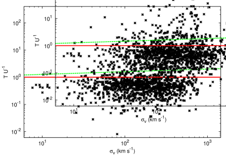
Figure 7: Virial ratio ($TU^{-1}$) versus the velocity dispersion ($\sigma_{v}$) of a group (in km s^-1). The rms straight line has been fitted to the data. The data are from the low-resolution $\Omega_{\Lambda}=0.73$ simulation when the apparent magnitude limit of $13.2$ has been adopted.

The weak trends are clearer if we scale the abscissa in both Figures 6 and 7 with the total mass of the group. Note that we use here the ’true’ mass of a group rather than the ’observable’ mass. Results are shown in Figures 8 and 9. More significant trends are now seen in both Figures, even-though the data are still scattered. The linear correlation coefficient of $0.32$ suggests that a significant correlation exists between the number of haloes and the virial ratio when the first is scaled with the total mass of the group. The correlation in Figure 8 is significant at level of $0.001$ and $P(r)<10^{-25}$. The slope of the rms line in Figure 8 is $b=0.82\pm 0.03$.

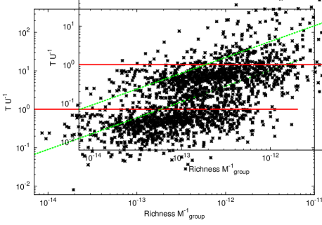
Figure 8: Virial ratio ($TU^{-1}$) versus the number of members (Richness) in a group when the latter has been scaled with the total mass of the group (M${}^{-1}_{group}$ in $h^{-1}~{}M_{\odot}$). The rms straight line has been fitted to the data. The data are from the low-resolution $\Omega_{\Lambda}=0.73$ simulation when the apparent magnitude limit of $13.2$ has been adopted.

Figure 9 shows a strong trend even-though the data are still quite scattered. The linear correlation coefficient of $0.40$ suggests that the correlation between the velocity dispersion of a group and the virial ratio of a group is quite strong. The correlation in Figure 9 is significant at level of $0.001$ and $P(r)<10^{-25}$. The slope with standard errors of the rms line is now $b=0.90\pm 0.03$.

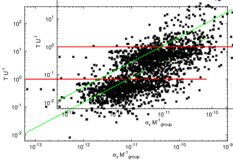
Figure 9: Virial ratio ($TU^{-1}$) versus the velocity dispersion ($\sigma_{v}$) of a group (in km s^-1) when the latter has been scaled with the total mass of the group (M${}^{-1}_{group}$ in $h^{-1}~{}M_{\odot}$).The rms straight line has been fitted to the data. The data are from the low-resolution $\Omega_{\Lambda}=0.73$ simulation, when the apparent magnitude limit of $13.2$ has been adopted.

When the apparent magnitude limit is changed to $20.0$, the trends of Figures 8 and 9 become stronger and the asymptotic standard errors for the rms lines become much smaller. The linear correlation coefficient of $0.62$ shows that the correlation between the velocity dispersion of a group, and the virial ratio, is strong when the apparent magnitude limit of $20.0$ is adopted. This correlation is significant at level of $0.001$ and $P(r)<10^{-25}$. What might be surprising is that changing the cosmological model, i.e. the value of the cosmological constant $\Omega_{\Lambda}$, does not have a substantial influence on Figures 9 and 10. The number of groups found from different simulations varies a lot as a function of $\Omega_{\Lambda}$ but the fraction of gravitationally bound groups do not (see Table 6). For comparison with Figures 8 and 9, we show results from the $\Omega_{\Lambda}=0.0$ simulation in Figures 10 and 11. In these figures the apparent magnitude limit of $20.0$ has been adopted. Otherwise, Figures 10 and 11 are comparable to Figures 8 and 9. The linear correlation coefficient in Figures 10 and 11 is: $0.32$ and $0.65$, respectively. Both of the correlations are significant at a level of $0.001$ and $P(r)<10^{-25}$ for both samples. The asymptotic standard errors for the rms lines in Figures 10 and 11 are small: $b=0.83\pm 0.02$ and $b=0.91\pm 0.01$, respectively.

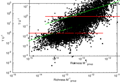
Figure 10: Virial ratio ($TU^{-1}$) versus the number of members in a group (Richness) when the latter has been scaled with the total mass of a group (M${}^{-1}_{group}$ in $h^{-1}~{}M_{\odot}$), and $\Omega_{\Lambda}=0.0$ and $m_{lim}=20.0$ has been adopted. The rms straight line has been fitted to the data.

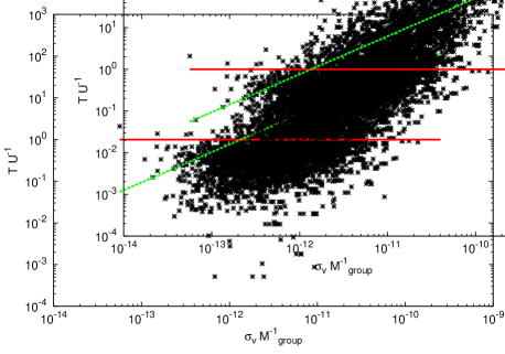
Figure 11: Virial ratio ($TU^{-1}$) versus the velocity dispersion ($\sigma_{v}$) of a group (in km s^-1) when the latter has been scaled with the total mass of a group (M${}^{-1}_{group}$ in $h^{-1}~{}M_{\odot}$), and $\Omega_{\Lambda}=0.0$ and $m_{lim}=20.0$ has been adopted. Straight line is a rms fit to the data.

7 Discussion

7.1 Probability functions of unbound groups

In this subsection we briefly discuss a method, which gives a theoretical probability of a group being gravitationally unbound. The mass of the groups is assumed to be known. In observations, estimations of group masses are less than precise at best, therefore the applicability of this method to observational data is merely hypothetical. The observable quantities we study are the velocity dispersion divided by the group mass $\sigma_{v}M_{group}^{-1}$ and the mean pairwise separation divided by the group mass $R_{P}M_{group}^{-1}$.

To calculate the probability functions for the groups, the first step is to choose an appropriate bin length (generally between $0.15$ and $0.30$) in the logarithm of the observable quantity. Then one calculates the number of groups and the number of gravitationally bound groups in each bin and divides the number of unbound groups with the total number of groups in the bin. The logarithmic scale is chosen in order to lower the dispersion of the data and to assure a large enough number of groups in every bin.

The probability functions for the velocity dispersion $\sigma_{v}$ and the mean pairwise separation $R_{p}$, normalised to the group mass, are shown in Figures 12 and 13. Figure 12 shows that at values larger than $1.8$ (the horizontal dotted line in Figure 12) it is more probable that the groups are gravitationally unbound when the $\Omega_{\Lambda}=0.73$ model is adopted. The same result can also be inferred from Figure 9, but with lower confidence.

The $\Omega_{\Lambda}=0.0$ simulation gives a probability function which is comparable to the probability function of the $\Omega_{\Lambda}=0.73$ model. It shows a similar linear growth as the probability function of the $\Omega_{\Lambda}=0.73$ model. However, the function is shifted along the horizontal axis. This shifting originates from the variation of the group masses and velocity dispersions (see Figure 5). The change of the apparent magnitude limit does not have any significant effect on Figure 12. When the apparent magnitude limit of $13.2$ is adopted, a smaller number of haloes and groups are observed, which enlarges the variations between bins and gives a worse fit to a straight line.

The quantity $\sigma_{v}$M${}^{-1}_{group}$, studied in Figure 12, has a loose connection to the kinetic energy $T$. This connection explains the fact that the lower normalized values of the quantity $\sigma_{v}$M${}^{-1}_{group}$ gives gravitationally bound groups with a higher probability, and larger normalized values, loosely meaning the larger kinetic energies, gives unbound groups with a higher probability.

Figure 12: Unbound probability ($P(TU^{-1}>1.0)$) versus velocity dispersion ($\sigma_{v}$) of a group when the $\Omega_{\Lambda}=0.73$ model, the apparent magnitude limit of $20.0$, and a bin length of $0.2$ are adopted. $\sigma_{v}$M${}^{-1}_{group}$ is in units of km s^-1 $(10^{12}h^{-1}~{}M_{\odot})^{-1}$.

The probability function of the mean pairwise separation (Figure 13) shows a similar linear growth as the probability function of the velocity dispersion in Figure 12. The variation from bin to bin is somewhat larger in the probability function of the mean pairwise separation due to the fact that the mean pairwise separation is not strictly the size of the group but it includes projection effects. The quantity $R_{p}$M${}^{-1}_{group}$, studied in Figure 13, is inversely proportional to the potential energy $U$ if the mean pairwise separation is identified as the real size of a group. The difference between Figures 12 and 13 is understandable, as the velocity dispersion and the mean pairwise separation are not strictly connected to each other, although some loose relation exists as the equation of the mean pairwise separation includes the mean group radial velocity.

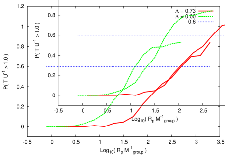
Figure 13: Unbound probability ($P(TU^{-1}>1.0)$) versus mean pairwise separation ($R_{p}$) when the $\Omega_{\Lambda}=0.73$ model, the apparent magnitude limit of $20.0$, and a bin length of $0.25$ are adopted. $R_{p}$M${}^{-1}_{group}$ is in units of Mpc $(10^{15}h^{-1}~{}M_{\odot})^{-1}$.

The $\Omega_{\Lambda}=0.90$ simulation show similar probability functions as the $\Omega_{\Lambda}=0.0$ and the $\Omega_{\Lambda}=0.73$ simulations. Figures 12 and 13 show that the $\Omega_{\Lambda}$ does not have any significant effect for the fraction of gravitationally unbound groups. This result can also be inferred from Table 6. The small effect is hardly surprising as the theoretical studies (see e.g. Lahav et al. 1991) have predicted that the $\Omega_{\Lambda}$ has little effect on the dynamics at the present epoch.

8 Conclusions

We have shown that the $\Lambda$CDM cosmology can produce groups of dark matter haloes comparable to observations of groups of galaxies when the FOF algorithm based on that of Huchra & Geller (1982) is adopted and the dynamical properties of groups are studied. Our groups from cosmological simulations are, in general, in a moderate agreement with observations, although a straight K-S test fails in most cases. Our $\Omega_{\Lambda}=0.73$ simulations are in satisfactory agreement with observations as the number densities of group properties are usually within 2$\sigma$ errors, or less, from the HG82 and the UZC-SSRS2 group abundances. The agreement between simulations and observations is good when the velocity dispersion and the ’observable’ mass of groups is considered. In these cases the applied K-S test is approved when the high resolution $\Omega_{\Lambda}=0.73$ simulation is considered. The moderate agreement between simulations and observational data suggests that gravitational force alone is sufficient in order to explain the dynamical properties of groups of galaxies.

We have also shown that in general about $20$ per cent of the groups of haloes generated with the algorithm presented in the HG82 are not gravitationally bound objects. The fraction of gravitationally bound groups of dark matter haloes varies with different values of the apparent magnitude limits. When the apparent magnitude limit is raised from the original $13.2$ to $20.0$, a larger number of spurious groups are found. The larger fraction of unbound groups with $m_{lim}=20.0$ could be explained by the fact that more interlopers are included into groups, when the apparent magnitude limit is increased. However, this analysis is beyond the scope of this study.

In general, a larger number of ’rich’ groups are found when the apparent magnitude limit is lowered. This originates from the fact that more light haloes at close proximity to more massive haloes become visible and those light haloes are included into the groups. When the magnitude limit is raised from the original value of $13.2$ to $12.0$, a slightly larger fraction of the groups are found to be gravitationally bound. In general, fewer groups (in absolutely number) are found and these groups are ’poorer’.

Small differences are found when the fractions of gravitationally bound ’poor’ and ’rich’ groups are studied. ’Rich’ groups with more than four members are more often gravitationally bound than ’poorer’ groups. This result agrees with previous ones (e.g. Ramella et al. 2002). Our results do not confirm the claim by Ramella et al. (1997) who argued that 50 to 75 per cent of groups with three members are spurious. Our results show that $\sim 77$ per cent of groups containing only three members are gravitationally bound when the apparent magnitude limit of $13.2$ is adopted.

When the value of the cosmological constant $\Omega_{\Lambda}$ is varied, the fractions of unbound groups change only slightly. This is somewhat surprising as it would be intuitively expected that a larger value of the dark energy would lead to a greater number of groups that are not gravitationally bound. Some variation is observed when the fraction of gravitationally bound groups is studied as a function of the cosmological constant, but, in general, a significant number of groups remains unbound in all cases of $\Omega_{\Lambda}$.

When the values of the free parameters of the FOF algorithm are varied, the fraction of gravitationally bound groups can be raised from $\sim 81$ to $\sim 83$ per cent. A greater difference is observed when the fraction of isolated haloes is studied. Varying the values of $D_{0}$ and $V_{0}$ makes a great difference, raising the fraction of isolated haloes from $\sim 42$ to $\sim 65$ per cent. In general, we do not find any significant difference in the fractions of gravitationally bound groups when different values of $D_{0}$ and $V_{0}$ or parameters of the Schechter luminosity function are adopted.

In observations, the crossing time of a group is often taken as an indicator of the virialization. We do not find any correlation between the virial ratio and the crossing time of a group. This result does not depend on the chosen value of the apparent magnitude limit of the search, or the cosmological model adopted. The lack of the correlation between these two variables calls into question the crossing time as an estimator of the virialization.

References

- Aceves & Velázquez (2002) Aceves H., Velázquez H., 2002, Revista Mexicana de Astronomia y Astrofisica, 38, 199
- Berlind et al. (2006) Berlind A.A., Frieman J., Weinberg D.H., Blanton M.R., Warren M.S., Abazajian K., Scranton R., Hogg D.W., Scoccimarro R., Bahcall N.A., Brinkmann J., Gott J.R.I., Kleinman S.J., Krzesinski J., Lee B.C., Miller C.J., Nitta A., Schneider D.P., Tucker D.L., Zehavi I., 2006, ApJS, 167, 1
- Byrd & Valtonen (1985) Byrd G.G., Valtonen M.J., 1985, ApJ, 289, 535
- Carlberg et al. (2001) Carlberg R.G., Yee H.K.C., Morris S.L., Lin H., Hall P.B., Patton D.R., Sawicki M., Shepherd C.W., 2001, ApJ, 552, 427
- Casagrande & Diaferio (2006) Casagrande L., Diaferio A., 2006, MNRAS, 373, 179
- Chernin & Mikkola (1991) Chernin A.D., Mikkola S., 1991, MNRAS, 253, 153
- Cooray & Milosavljević (2005) Cooray A., Milosavljević M., 2005, ApJ, 627, L89
- Cox (2000) Cox A.N., 2000, Allen’s astrophysical quantities, 4th ed. Publisher: New York: AIP Press; Springer.
- de Vaucouleurs (1958) de Vaucouleurs G., 1958, AJ, 63, 253
- Diaferio et al. (1993) Diaferio A., Ramella M., Geller M.J., Ferrari A., 1993, AJ, 105, 6
- Diaferio et al. (1994) Diaferio A., Geller M.J., Ramella M., 1994, AJ, 107, 3
- Diaferio et al. (1999) Diaferio A., Kauffmann G., Colberg J.M., White S.D.M., 1999, MNRAS, 307, 537
- Driver et al. (2007) Driver S.P., Allen P.D., Liske J., Graham A.W., 2007, ApJ, 657, L85
- Eke et al. (2004) Eke V.R., Baugh C.M., Cole S., Frenk C.S., Norberg P., Peacock J.A., Baldry I.K., Bland-Hawthorn J., Bridges T., Cannon R., Colless M., Collins C., Couch W., Dalton G., de Propris R., Driver S.P., Efstathiou G., Ellis R.S., Glazebrook K., Jackson C., Lahav O., Lewis I., Lumsden S., Maddox S., Madgwick D., Peterson B.A., Sutherland W., Taylor K. 2004, MNRAS, 348, 866
- Ekholm et al. (2001) Ekholm T., Baryshev Y., Teerikorpi P., Hanski M. & Paturel G., 2001, A&A, 368, L17
- Frederic (1995a) Frederic J.J., 1995a, ApJS, 97, 259
- Frederic (1995b) Frederic J.J., 1995b, ApJS, 97, 275
- Geller & Huchra (1983) Geller M.J., Huchra J.P., 1983, ApJS, 52, 61
- Gill et al. (2004) Gill S.P.D., Knebe A., Gibson B.K., 2004, MNRAS, 351, 399
- Girardi et al. (1992) Girardi M., Mezzetti M., Giuricin G., Mardirossian F., 1992, ApJ, 394, 442
- Giudice (1999) Giudice G., 1999, ASPC, 176, 136
- Giuricin et al. (2000) Giuricin G., Marinon C., Ceriani L., Pisani A., 2000, ApJ, 543, 178
- Gott & Turner (1977) Gott III J.R., Turner E.L., 1977, ApJ, 213, 309
- Gourgoulhon et al (1992) Gourgoulhon E., Chamaraux P., Fouqué P., 1992, A&A, 255, 69
- Holmberg (1950) Holmberg E. 1950, Medd. Lunds Obs. Ser.2, 128
- Huchra & Geller (1982) Huchra J.P., Geller M.J., 1982, ApJ, 257, 423 (HG82)
- Humason et al. (1956) Humason M.L., Mayall N.U., Sandage A.R., 1956, ApJ, 61, 97
- Iovino & Hickson (1997) Iovino A., Hickson P., 1997, MNRAS, 287, 21
- Klypin et al. (2003) Klypin A., Hoffman Y., Kravtsov A.V., Gottlöber S., 2003, ApJ, 596, 19
- Knebe et al. (2001) Knebe A., Green A., Binney J., 2001, MNRAS, 325, 845
- Lahav et al. (1991) Lahav O., Lilje P.B., Primack J.R., Rees M.J., 1991, MNRAS, 251, 128
- Macció et al. (2005) Macció A.V., Governato F., Horellou C., 2005, MNRAS, 359, 941
- Merchán & Zandivarez (2002) Merchán M., Zandivarez A., 2002, MNRAS, 335, 216
- Moore et al. (1993) Moore B., Frenk C.S., White S.D.M., 1993, MNRAS, 261, 827
- Nolthenius & White (1987) Nolthenius R.A., White S.D.M., 1987, MNRAS, 235, 505
- Nolthenius et al. (1997) Nolthenius R., Klypin A.A., Primack J.R., 1997, ApJ, 480, 43
- Oguri (2006) Oguri M., 2006, MNRAS, 367, 1241
- Peirani & de Freitas Pacheco (2006) Peirani S., de Freitas Pacheco J.A., 2006, NewA, 11, 325
- Plionis et al. (2006) Plionis M., Basilakos S., Ragone-Figueroa C., 2006, ApJ, 650, 770
- Ramella et al. (1989) Ramella M., Geller M.J., Huchra J.P., 1989, ApJ, 344, 57
- Ramella et al. (1997) Ramella M., Pisani A., Geller M.J., 1997, AJ, 113, 483
- Ramella et al. (2002) Ramella M., Geller M.J., Pisani A., da Costa L.N., 2002, AJ, 123, 2976
- Sandage (1999) Sandage A., 1999, ApJ, 527, 479
- Sandage & Tammann (1975) Sandage A., Tammann G.A., 1975, ApJ, 196, 313
- Schechter (1974) Schechter P., 1974, ApJ, 203, 557
- Sulentic (1984) Sulentic J., 1984, ApJ, 286, 542
- Teerikorpi et al. (2005) Teerikorpi P., Chernin A.D., Baryshev Yu.V., 2005, A&A, 440, 791
- Tucker et al. (2000) Tucker D.L., Oemler A.J., Hashimoto Y., Shectman S.A., Kirshner R.P., Lin H., Landy S.D., Schechter P.L., Allam S.S., 2000, ApJS, 130, 237
- Vale & Ostriker (2004) Vale A., Ostriker J.P., 2004, MNRAS, 353, 189
- Valtonen & Byrd (1986) Valtonen M.J., Byrd G.G., 1986, ApJ, 303, 523