A deeply embedded young protoplanetary disk around L1489 IRS observed by the Submillimeter Array

Abstract

Context. Circumstellar disks are expected to form early in the process that leads to the formation of a young star, during the collapse of the dense molecular cloud core. It is currently not well understood at what stage of the collapse the disk is formed or how it subsequently evolves.

Aims. We aim to identify whether an embedded Keplerian protoplanetary disk resides in the L1489 IRS system. Given the amount of envelope material still present, such a disk would respresent a very young example of a protoplanetary disk.

Methods. Using the Submillimeter Array (SMA) we have observed the HCO⁺ $J=$ 3–2 line with a resolution of about 1^′′. At this resolution a protoplanetary disk with a radius of a few hundred AUs should be detectable, if present. Radiative transfer tools are used to model the emission from both continuum and line data.

Results. We find that these data are consistent with theoretical models of a collapsing envelope and Keplerian circumstellar disk. Models reproducing both the SED and the interferometric continuum observations reveal that the disk is inclined by 40^∘ which is significantly different to the surrounding envelope (74^∘).

Conclusions. This misalignment of the angular momentum axes may be caused by a gradient within the angular momentum in the parental cloud or if L1489 IRS is a binary system rather than just a single star. In the latter case, future observations looking for variability at sub-arcsecond scales may be able to constrain these dynamical variations directly. However, if stars form from turbulent cores, the accreting material will not have a constant angular momentum axis (although the average is well defined and conserved) in which case it is more likely to have a misalignment of the angular momentum axes of the disk and the envelope.

1 Introduction

Circumstellar disks constitute an integral part in the formation of low-mass protostars, being a direct result of the collapse of rotating molecular cloud cores and the likely birthplace of future planetary systems. When a molecular cloud core collapses to form a low-mass star, its initial angular momentum causes material to pile up on scales of $\sim 100$ AU in a circumstellar disk (Cassen & Moosman 1981; Terebey et al. 1984; Adams et al. 1987, 1988). Due to accretion processes as the young stellar object (YSO) evolves, the disk grows in size while the envelope dissipates (e.g., Basu 1998; Yorke & Bodenheimer 1999). In the more evolved stages of young stellar objects such disks can be imaged directly at optical and near-infrared wavelengths (e.g., Burrows et al. 1996; Padgett et al. 1999) and their chemical and dynamical properties can be derived from comparison to submillimeter spectroscopic observations (e.g., Thi et al. 2001). Still, this latter method is often not unique, but requires a priori assumptions about the underlying disk structure. In the earlier embedded stages this method is even more complex, because the disk is still deeply embedded in cloud material so that any signature of rotation in the disk itself, for example, is smeared out by emission that originates in the still collapsing envelope. By going to higher resolution using interferometric observations, as well as observing high density gas tracers, more reliable detections of protoplanetary disks can be made as direct imaging is approached (Rodríguez et al. 1998; Qi et al. 2004; Jørgensen et al. 2005b). In this paper we present such high-angular resolution submillimeter wavelength observations from the Submillimeter Array (SMA) of the embedded YSO L1489 IRS. We show how these observations place strong constraints on its dynamical structure and evolutionary status through detailed modeling.

L1489 IRS (IRAS 04016+2610) is an intriguing protostar in the Taurus star forming region ($d=140$ pc) classified as a Class I YSO according to the classification scheme of Lada & Wilking (1984). It is still embedded in a large amount of envelope material in which a significant amount of both infall and rotation has been observed on scales ranging from a few tenths of an AU out to several thousands of AUs (Hogerheijde 2001; Boogert et al. 2002). This large degree of rotation makes this source an interesting case study for the evolution of angular momentum during the formation of low-mass stars, potentially linking the embedded (Class 0 and I) and revealed (Class II and III) stages.

In a recent study by Brinch et al. (2007) (referred to as Paper I), a model of L1489 IRS was presented based on data from a large single-dish molecular line survey (Jørgensen et al. 2004). This study was motivated by the intriguing peculiarities seen in L1489 IRS, such as the unusual large size and shape of the circumstellar material. The aim was to constrain the structure of its larger-scale infalling envelope and to place it in the right context of the canonical picture of low-mass star formation (see for example several reviews in Reipurth et al. 2007).

The model presented in Paper I describes a flattened envelope with an inspiraling velocity field, parameterized by the stellar mass and the (constant) angle of the field lines with respect to the azimuthal direction. A spherical temperature profile was adopted and the model did not explicitly contain a disk. The mass of the envelope is 0.09 M_⊙, adopted from Jørgensen et al. (2002). The use of such a “global” model is sufficient when working with single-dish data, where the emission is dominated by the emission from the large-scale envelope. With this description it was possible to accurately reproduce all the observed single-dish lines.

What the study of Paper I could not address, is whether a rotationally dominated disk is present on scales of the order of hundreds of AUs, although the amount of rotation which is inferred by the single-dish observations certainly suggests that a disk should have formed. In addition, two specific puzzles remain about the structure of L1489 IRS inferred on basis of the model when compared to other studies in the literature. First, the best fit was obtained with a central mass of 1.35 M_⊙, which is a very high value given that the luminosity of the star has been determined to be only 3.7 L_⊙ (Kenyon et al. 1993). Second, it was found that the best fit inclination of the system was 74^∘. This is in agreement with the result from Hogerheijde (2001) where they showed that in order to reproduce the observed aspect ratio the inclination cannot be less than 60^∘. However, in a recent study, Eisner et al. (2005), modeled the spectral energy distribution (SED) of L1489 IRS and demonstrated that this required a significantly different systemic inclination of only 36^∘.

In this paper, we try to address these issues through arc second scale interferometric observations of the dense gas tracer HCO⁺ $J=3-2$ from the Submillimeter Array. These observations provide information on the gas dynamics on scales $\sim$100 AU and reveal an embedded protoplanetary disk. We show how careful modeling of the full SED from near-infrared through millimeter wavelengths can place strong constraints on the geometry of such a disk.

The outline of this paper is as follows: Sect. 2 describes the details of the observations and data reduction while Sect. 3 presents the data. Sect. 4 introduces our model in which we have now included a disk and we also show how this model can fit all available observations including our new SMA data. Finally, in Sect. 5 and 6 we discuss the implications of our model and summarize our results.

2 Observations and data reduction

Observations were carried out at the Submillimeter Array (SMA) located on Mauna Kea, Hawaii. Our data set consists of two separate tracks of measurements in different array configurations. The first track was obtained on December 11, 2005. This track was done in the compact configuration resulting in a spatial resolution of $\sim$ 2.5^′′ with projected baselines ranging between 10 and 62 k$\lambda$. A second track was obtained on November 28, 2006, in the extended configuration with the resolution of about 1^′′ and baselines between 18 and 200 k$\lambda$. The resolution of the two configurations corresponds to linear sizes of 350 AU and 140 AU respectively. The synthesized beam size of the combined track using uniform visibility weighting is 0.9${}^{\prime\prime}\times$ 0.7^′′ with a position angle of 78^∘.

In both tracks the receiver was tuned to HCO⁺ $J=$ 3–2 at 267.56 GHz. We used a correlator configuration with high spectral resolution across the line, providing a channel width of 0.2 kms^-1 over 0.104 GHz. The remainder of the 2 GHz bandwidth of the SMA correlator was used to measure the continuum. No other lines in this band are expected to contaminate the continuum. We did not encounter any technical problems during observations and the weather conditions were excellent during both tracks. For the compact configuration track, $\tau_{225}$ was 0.06 and for the extended track $\tau_{225}$ was at 0.08.

Mars was used as flux calibrator in the first track, and Uranus for the second track. The quasars 3c454.3, 3c273, and 3c279 were used for passband calibration for both tracks, while the complex gains were calibrated using the two quasars 3c111 and 3c84 located within 18 degrees from L1489 IRS. The calibrators were measured every 20 minutes throughout both tracks. Their fluxes have been determined to be 3.1 and 2.6 Jy for 3c111 and 3c84 in the compact track, and 2.3 and 2.2 Jy respectively in the extended track. For the gain calibration, a time smoothing scale of 0.7 hours was used which ensures that the large scale variations in the phase during the track are corrected for. The data do not show any significant small scale variations (i.e., rapid fluctuations in the phases or amplitudes). The quasars appear as point sources even at the longest baselines, which means that phase decorrelation due to atmospheric turbulence is negligible. The signal-to-noise of the calibrators is $>$50 per integration.

The data were reduced using the MIR software package (Qi 2005). Due to the excellent weather conditions, the data quality is very high and the data reduction procedure went smooth and unproblematic. All post-processing of the data, including combining the two visibility sets was done using the MIRIAD package (Sault et al. 1995). Relevant numbers are presented in Table 1.

In this paper we also make use of continuum measurements of L1489 IRS found in the literature ranging from the near-infrared (Kenyon et al. 1993; Eisner et al. 2005; Padgett et al. 1999; Park & Kenyon 2002; Whitney et al. 1997; Myers et al. 1987; Kessler-Silacci et al. 2005) to (sub)millimeter wavelengths (Hogerheijde & Sandell 2000; Moriarty-Schieven et al. 1994; Motte & André 2001; Hogerheijde et al. 1997; Ohashi et al. 1996; Saito et al. 2001; Lucas et al. 2000).

Table 1: Summary of the SMA observations.

Source	L1489 IRS
$\alpha,\delta$(2000)a	04:04:42.85, +26:18:56.3
Frequency	267.55762 GHz (1.12 mm)
Integrated line intensity	41.85 Jy beam-1 km s-1
Peak line intensity	2.04 K
Noise level (rms)	0.35 Jy beam-1
Continuum flux	36.0$\pm$2.3 mJy
Noise level (rms)	3.7 mJy beam-1
Synthesized beam size	$0.9^{\prime\prime}\times 0.7^{\prime\prime}$
(Uniform weighting)

^a Coordinates are given at the position where the continuum emission peaks.

3 Results

The two tracks of observations provide us with two sets of $(u,v)$–points which, when combined and Fourier transformed, samples the image $(x,y)$ plane well from scales of 1 to 30^′′ (140 to 4200 AU). Emission on spatial scales greater than this is filtered out by the interferometer due to its finite shortest spacing. This filtering is accounted for when comparing models to the observations.

The measured continuum emission is shown as an image in Fig. 1. Previous attempts to measure the continuum at 1.1 mm with the BIMA interferometer were not successful (Hogerheijde 2001). The SMA however, reveals a complex and detailed, slightly elongated, structure.

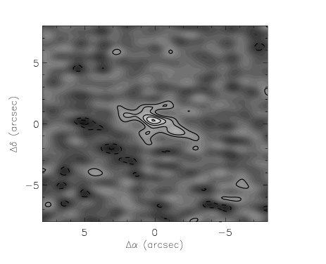
Figure 1: Reconstructed image of the continuum emission at the highest resolution (0.9${}^{\prime\prime}\times$ 0.7^′′). The contours are linearly spaced with 1$\sigma$ starting at 2$\sigma$ and dashed lines are negative contour levels.

Two reconstructed images of the HCO⁺ emission are shown in Fig. 2 using the natural and uniform weighting schemes, optimizing the signal-to-noise and angular resolution, respectively. In this figure, the zero moment map is plotted as solid contour lines and the first moment is shown as shaded contours. It is clear that both images reveal an elongated, flat structure. In the uniformly weighted image there is a large amount of asymmetry in the structure, which is less prominent in the naturally weighted image.

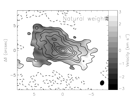
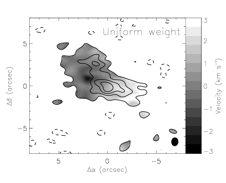
Figure 2: Zero and first moment plots of the HCO⁺ $J=$ 3–2 emission toward L1489 IRS. Contours are linearly spaced by 2$\sigma$ with a clip level of 2$\sigma$. $\sigma$ equals 1.1 and 2.0 Jy bm^-1 km s^-1 for the natural and uniform weighting schemes respectively. Negative contours appear as dashed lines.

The velocity contours in the lower panel of Fig. 2 are seen to be closed around a point which is offset with some 3^′′ from the peak of the emission. There is also clearly a gradient in the velocity field along the major axis of the object. This feature was previously reported by Hogerheijde (2001) using interferometric observations of HCO⁺ $J=$ 1–0, and low S/N HCO⁺ $J=$ 3–2 observations, from the BIMA and OVRO arrays. The gradient in the velocity field coincides almost perfectly with the long axis of the structure. When compared to the BIMA HCO⁺ $J=$ 3–2 observations, the SMA data give 5–10 times better resolution. Furthermore, the BIMA data had to be self-calibrated using the HCO⁺ $J=$ 1–0 image as a model and thus the resulting image was somewhat dependent of the structure of the lower excitation emission. The image we obtain from the SMA data is of considerably better quality.

In Fig. 3, the zero moment emission contours have been superposed on the near-infrared scattered light image taken by the Hubble Space Telescope (Padgett et al. 1999). The figure shows that many of the details in the SMA image coincide with features seen in the scattered light image.

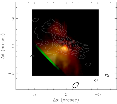
Figure 3: HCO⁺ emission (1$\sigma$) contours superposed on the near-infrared scattered light image (Padgett et al. 1999).

The spectral map in Fig. 4 shows single spectra at positions offset by 2^′′ from each other. Each position shown here is the spectrum contained within one synthesized beam. The center most spectrum coincides with the peak of the emission in Fig. 2. Here is seen a very broad, double peaked line. Moving outward from the center, the lines become single peaked and offset in velocity space with respect to the systemic velocity. Perpendicular to the long axis of the structure, the line intensity falls off quickly. The lines shown in Fig. 4 are reconstructed using the natural weighting scheme. For the remainder of this paper we will use the uniformly weighted maps where the resolution is optimal.

Figure 4: Spectral map of L1489 IRS. The spectra are evenly spaced with 2^′′. The bandwidth in each panel is 20 kms^-1. The scale on the $y$-axis goes from 0 to 2 Jybm^-1.

Fig. 5 shows the emission in a position-velocity diagram, where the image cube has been sliced along the major axis to produce the intensity distribution along the velocity axis. The PV–diagram shows almost no emission in the second and fourth quadrant which is a strong indicator of rotation. The small amount of low velocity emission seen close to the center in the fourth quadrant may be accounted for by infalling gas.

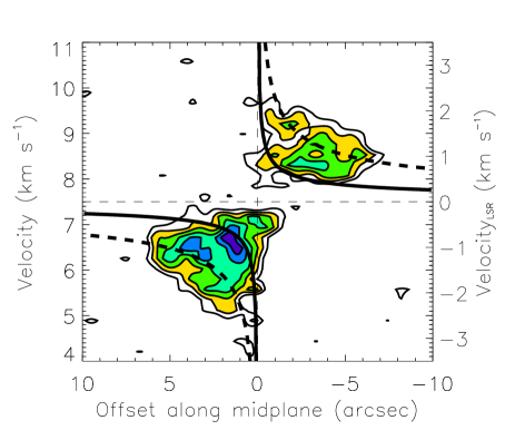
Figure 5: Position-Velocity (PV) diagram. This plot shows that the emission on the scales measured by the SMA is entirely dominated by rotation. The black curves show the Keplerian velocity, calculated from the dynamic mass (1.35 M_⊙) obtained in Paper I. The curves have been inclination corrected with 74^∘ for the full lines and 40^∘ for the dashed lines. Contours start at 2$\sigma$ and increase with 1$\sigma$ = 0.12 Jy beam^-1.

4 Analysis

With the resolution provided by the SMA it is possible to probe the central parts of L1489 IRS on scales of $\sim$100 AU, where the protoplanetary disk is expected to be present (see Section 1). Furthermore, the HCO⁺ $J=$ 3–2 transition traces H₂ densities of $10^{6}$ cm^-3 or more (Schöier et al. 2005), which are expected in the inner envelope and disk. The model of Paper I was not explicitly made to mimic a disk, but rather to describe the morphology of the images on large scales. Using this model, which works well on a global scale, we can explore how well it fits the SMA spectra when extrapolated to scales unconstrained by the single-dish observations.

Fig. 6 compares the SMA observations to the predictions of this model (dashed line). For doing this comparison, the model is imaged using the $(u,v)$-spacings from the observations, so that directly comparable spectra are obtained. While the spectra away from the center are fairly well reproduced in terms of line width, the center position is too wide, i.e., the model produces velocities that are too extreme compared to the measured velocities.

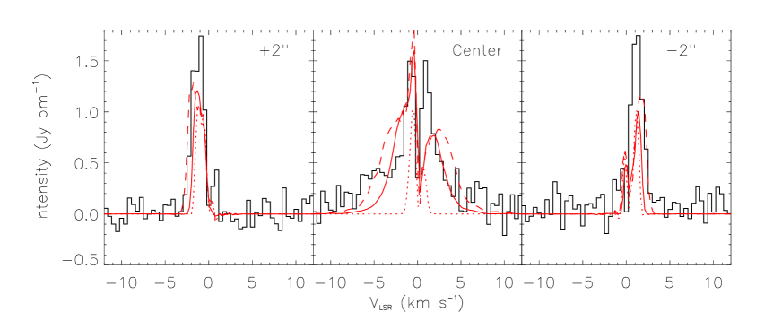
Figure 6: This figure shows three spectra from the SMA observations with model spectra superposed. The two off-positions are chosen in the direction along the long axis of the object. The offsets are chosen to be a resolution element. Three models are also shown: The dashed line shows the unmodified model from Paper I, the full line is the model from Paper I, but inclined at 40^∘, and the dotted line shows a model where HCO⁺ is absent on scales smaller than 200 AU.

To check that this emission does in fact originate from scales less than 200 AU, a model where HCO⁺ is completely absent within a radius of 200 AU is also shown in Fig. 6 with the dotted line. In this model the wide wings disappear and only a very narrow line is left. The two off-positions, which lie outside of the radius of 200 AU, are not affected minimally introducing this cavity.

Fig. 6 also shows a spectrum which is made from the Paper I model, but inclined at 40^∘ (full line). This is a considerably better fit than the other two models (again the two off-positions are little affected). While the observations of the larger scale structure (Paper I, Hogerheijde (2001)) demonstrates that the inclination of the flattened, collapsing envelope is $\sim$74^∘, the SMA observations suggest that a change in the inclination occurs on scales of 100–200 AU, reflecting a dynamically different component there. On the other hand, since the model of Paper I was tuned to match the single-dish observation on scales of $\sim$1000 AU or more and did not explicitly take the disk into account it is not unexpected that it does not fully reproduce the SMA observations.

4.1 Introducing a disk model

To reproduce also the interferometric observations we have modified the model from Paper I on scales corresponding to the innermost envelope and disk: The improvements consists largely of two things, namely a different parameterization of the density distribution and the explicit inclusion of a disk.

The description used in Paper I has a discontinuity for small values of $r$ and $\theta$: again, this is not a problem when working with the large scale emission, but becomes a problem when interfaced with a disk where a continuous transition from envelope to disk is preferred. The new parameterization we use for the envelope is adopted from Ulrich (1976). In this representation the envelope density is given by,

$$\rho_{env}(r,\theta) = \rho_{0}\left(\frac{r}{R_{rot}}\right)^{-1.5}\left(1+\frac{\cos\theta}{\cos\theta_{0}}\right)^{-1/2}$$ (1)

$$\times\left(\frac{\cos\theta}{2\cos\theta_{0}}+\frac{R_{rot}}{r}\cos 2\theta_{0}\right)^{-1},$$

where $\theta_{0}$ is the solution of the parabolic motion of an infalling particle given by $r/R_{rot}(\cos\theta_{0}-\cos\theta)/(\cos\theta_{0}\sin 2\theta_{0})=1$, $R_{rot}=150$ AU is the centrifugal radius of the envelope, and $\rho_{0}$ is the density on the equatorial plane and at the centrifugal radius. Since the outer radius, total mass, aspect ratio, and peak density are held fixed, the new parameterization is qualitatively similar to the Plummer-like profile used in Paper I. The numerical value of $R_{rot}$ is chosen so that the maximum deviation in density in the ($r,\theta$)-plane only reaches 20% in the most dense parts (outside of the disk cavity) and has an average deviation of less than 5%.

In addition to this envelope, a generic disk is also introduced in the model. The density of the disk is given by,

$$\rho_{disk}(r,\theta)=\frac{\Sigma_{0}\,(r/R_{0})^{-1}}{\sqrt{2\pi}\,H_{0}}\exp\left\{-\frac{1}{2}\left[\frac{r\,\cos\theta}{H_{0}}\right]^{2}\right\},$$ (2)

where $\theta$ is the angle from the axis of symmetry, $R_{0}$ is the disk outer radius and $H_{0}$ is the scale height of the disk. The model thus has four free parameters: disk radius, pressure scale height, mass (taken as a fraction of the total mass of the circumstellar material), and inclination. In order to maximize the mid-infrared flux, we use a flat disk, i.e., with no increase in scale height with radius and fix the scale height to 0.25. The outer radius is fixed to 200 AU, the distance from the center of the emission in Fig. 2 to the position of the closed velocity contour, thereby effectively reducing the number of free parameters to two. This outer disk radius is not a strongly constrained parameter since neither the SED nor the model spectra are influenced much by changes in this value. It is only possible to rule out the extreme cases, where the disk either gets so small that it is no longer influencing the SED or where it gets so big that it holds a significant fraction of the total mass. We find that the best fit is provided by a disk mass of $M_{disk}=4\times 10^{-3}$ M_⊙. A cross section of the model is shown in Fig. 7.

The velocity field in the envelope is similar to the one used in Paper I, where the velocity field was parameterized in terms of a central mass and an angle between the velocity vector and the azimuthal direction, so the the ratio of infall to rotation could be controlled by adjusting this angle. The best fit parameter values obtained in Paper I of 1.35M_⊙ for the central mass and flow lines inclined with 15^∘ with respect to the azimuthal direction, are used. No radial motions are allowed in the disk: only full Keplerian motion is present in the region of the model occupied by the disk.

In order to produce synthetic observations which can be directly compared to the data, we use numerical radiative transfer tools. The 3D continuum radiative transfer code RADMC (Dullemond & Dominik 2004) is used to calculate the scattering function and the temperature structure in the analytical axisymmetric density distribution. In these calculations, the luminosity measurement by Kenyon et al. (1993) of 3.7 L_⊙ is used for the central source. The solution is then “ray–traced” using RADICAL (Dullemond & Turolla 2000) to produce the spectral energy distribution and the continuum maps at the observed frequencies. In both RADMC and RADICAL we assume certain properties of the dust. We use the dust opacities that give the best fit to extinction measurements in dense cores (Pontoppidan et al., in prep).

The same density and temperature structure are afterward given as input to the excitation and line radiative transfer code RATRAN (Hogerheijde & van der Tak 2000) which is used to calculate the spatial and frequency dependent HCO⁺ $J=$ 3–2 emission. The HCO⁺ models are post-processed with the MIRIAD tasks uvmodel, invert, clean, and restore to simulate the actual SMA observations.

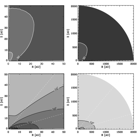
Figure 7: A slice through the model of L1489 IRS: The top panels show the temperature on different scales and the bottom panels show the corresponding density profiles.

4.2 Modeling the continuum emission

In Fig. 8, we compare our model to the continuum observations. We calculate $(u,v)$–amplitudes at 1.1 mm which we plot on top of the observed amplitudes. The result is in good agreement with the data, suggesting that the dust emission is well-described by our parameterization down to scales of $\sim$ 100 AU. This comparison is not very dependent on the inclination, since the continuum emission is quite compact. For this particular figure, an inclination of 40^∘ is assumed.

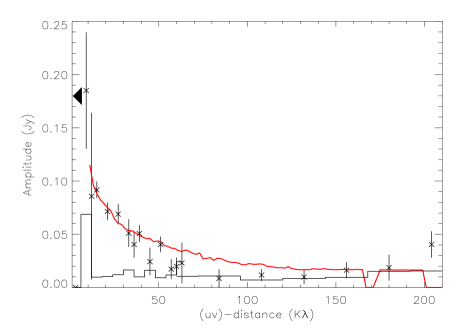
Figure 8: The averaged $(u,v)$–amplitudes of the continuum at 1 mm in both compact and extended configurations. The full line show our model. The compact configuration visibilities cover the $(u,v)$–distance up to 60 k$\lambda$. The black triangle marks the total flux at 1 mm (Moriarty-Schieven et al. 1994). The histogram indicates the zero-signal expectation values.

Recently, Eisner et al. (2005) modeled the SEDs of a number of Class I objects in Taurus including L1489 IRS. The model used in their work is parameterized differently from ours, but it essentially describes a similar structure. As pointed out above, Eisner et al. find a best fit inclination of 36^∘ in contrast to the inclination of 74^∘ found in Paper I.

To test the result of Eisner et al. (2005) we calculated the SED using the described model with only the system inclination as a free parameter (Fig. 9). The best fit is found for an inclination of about 40^∘, in good agreement with the result of Eisner et al. (2005). The models with inclinations of 50^∘ and 74^∘, are also plotted in Fig. 9 in order to show how the SED depends on inclination.

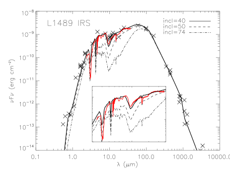
Figure 9: The model spectral energy distribution assuming inclinations of 40^∘ (full line) and 50^∘ and 74^∘ (broken lines) plotted on top of flux measurements from the literature (marked by crosses) and the Spitzer/IRS spectrum from 2 – 40 microns (red line).

Note that the quality of our best fit to the SED is comparable to the fit presented by Eisner et al. (2005), whereas the fit becomes rapidly worse with increasing inclination larger than 40^∘, thus bringing about disagreement with the results from (Hogerheijde 2001) and Paper I. The three different models plotted in Fig. 9 cannot be distinguished for wavelength above $\sim$60 $\mu$m, which corresponds to a temperature of about 40 K using Wiens displacement law. This temperature occurs on radial distances of approximately 100 AU from the central object which means that outside of this radius, the SED is no longer sensitive to the inclination. We interpret this behavior as a change in the angular momentum axis on disk scales, causing the disk to be inclined with respect to the envelope.

4.3 Modeling the HCO⁺ emission

In Paper I it was found that the characteristic double peak feature of the HCO⁺ $J=$ 4–3 line could not be reproduced with an inclination below 70^∘. On the other hand including a disk inclined by 40^∘ into the model of Paper I does not alter the fit to the single dish lines (Fig 10): the geometry and the velocity field of the material at scales smaller than $\sim$300 AU does not influence the shape of these lines. This fit is not perfect though as it still overestimates the red-shifted wing in the $J=$ 3–2 line and the width of the $J=$ 1–0 line slightly, but the quality of the fit is similar to that presented in Paper I.

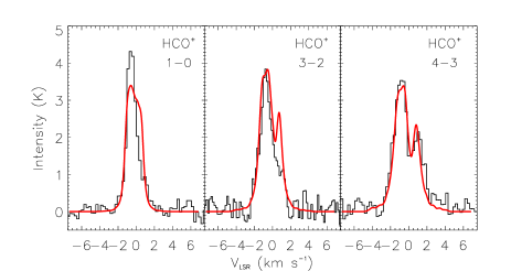
Figure 10: Three transitions of HCO⁺ observed by single-dish telescope (see Paper I for details) with our model superposed. The quality of the fit is comparable to the fit in Paper I although a disk model has now been included.

We need to test how well this tilted disk model works with the line observations from the SMA. It was shown in Sect. 4 that the off-position spectra are weakly dependent on changes in the inclination and that the same is true when using the model where the disk is tilted with respect to the envelope. The central position however, is seen in Fig. 11 to be very well reproduced in terms of line width and wing shape by this model. The model spectrum is slightly more asymmetric than the data, which means that the infall to rotation ratio is not quite correct on disk scales. The magnitude of the velocity field projected onto our line of sight is correct though, since the width of the line is well fit.

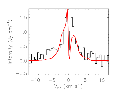
Figure 11: The SMA spectrum towards the center of L1489 IRS with our model, consisting of a disk which is inclined with respect to the envelope, superposed. As in Fig. 6, the model has been imaged with the $(u,v)$-spacings from the observations.

We also compared the averaged $(u,v)$–amplitudes to evaluate the quality of our model similar to the procedure for the continuum. Fitting the $(u,v)$–amplitudes in this way tests whether the model produces the right amount of emission at every scale. The best fit is shown in Fig. 12. The zero-spacing flux has been shown in this plot as well, marked by the black triangle. This method has previously been used to study the abundance variations of given molecules in protostellar envelopes, in particular imaging directly where significant freeze-out occurs in protostellar envelopes (Jørgensen 2004; Jørgensen et al. 2005a). The model does a good job reproducing the observed HCO⁺ brightness distribution on almost all scales with a constant abundance, except around 20–40 k$\lambda$ where it overestimates the amount of observed flux. This correspond to a radius of about 1000 AU, that is well outside of the disk. On the other hand single-dish observations of low-mass protostellar envelopes suggest that these are scales where significant freeze-out in particular of CO may occur at temperatures $\lesssim 20-30$ K, which because of the gas-phase chemical relation between CO and HCO⁺ also reflects directly in the observed distribution of HCO⁺ (e.g., Jørgensen et al. 2004, 2005b). Despite this, the difference between the model prediction and observations is small with this constant abundance, suggesting that the amount of freeze-out is small in L1489 IRS. This is in agreement with the single-dish studies of Jørgensen et al. (2002, 2004, 2005b), who generally found little depletion in the envelopes of L1489 IRS and other Class I sources in contrast to the more deeply embedded, Class 0, protostars.

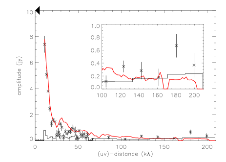
Figure 12: Similar to Fig. 8 but for the HCO⁺ $J=$ 3–2 measurements. The triangle marks the total flux obtained from the single dish observations. The amplitudes have been averaged over $\pm 5$ kms^-1 relative to the systemic velocity. The histogram indicates the zero-signal expectation values. The insert is an enlargement of the longest baselines.

The model parameter values obtained in this section including values from Paper I are summarized in Table 2. The best fit values that are derived in this paper are tuned by hand rather than systematically optimized by a $\chi^{2}$ minimization method. Therefore we can only give an estimate on the uncertainties. However, Fig. 9 shows that the SED fit gets rapidly worse when changing the inclination, and given the strong dependence of the envelope inclination on the single-dish lines, we estimate that both angles are accurate to within 10^∘. For the disk mass and radius, the uncertainties on the parameter values are less well defined for reasons given in Section 4.1, but we estimate an accuracy within a factor of 2 in each of these parameters.

Table 2: Model parameter values

Envelope	Value
Outer radiusa	2000 AU
Envelope massa	0.093 M⊙
Inclinationa,b	74∘
HCO+ abundancea	3.0$\times$10-9
Disk	Value
Radiusb	200 AU
Disk massb	4$\times$10-3 M⊙
Inclinationb	40∘
Scale heightc	z=0.25R
Central massa	1.35 M⊙
Central luminosityc	3.7 L⊙
Distancec	140 pc

^a Values from Paper I
^b Fitted values
^c Values adopted from the literature

5 Discussion

It seems that depending on the physical size scales that we probe, the solution favors a different inclination. When taking all available observations into account we need to introduce a model where the angular momentum vector of the disk is misaligned with the angular momentum vector of the (rotationally flattened) envelope. We adopt a two component model (illustrated in Fig. 13), disk and envelope, but in reality, the angular momentum axis may indeed be a continuous function of radius on the scales of the disk ($\lesssim$ a few hundred AU). The origin of such a misalignment can actually be explained in a simple way by considering the initial conditions of the collapse.

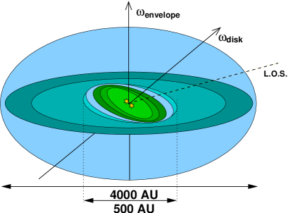
Figure 13: An (exaggerated) illustration of the proposed model where the angular momentum axis is changing with radius. The line of sight is illustrated by the dashed line.

The state of a pre-stellar core before the gravitational collapse begins is typically described by a static sphere with a solid body rotation perturbation (Terebey et al. 1984). Due to strict angular momentum conservation, such a model would be perfectly aligned throughout the collapse and consequently disk formation models are often described numerically by axisymmetric representations (e.g., Yorke & Bodenheimer 1999).

However, there is no a priori reason why a pre-stellar core should rotate as a solid body. Of course the cloud has an average angular momentum which on a global scale determines the axis of rotation. The cloud does not collapse instantly to form a disk though, but rather from the inside and out as described by Shu (1977), and therefore a shell of material from deep within the cloud, which may very well have an average angular momentum that is different from the global average, will collapse and form a disk before material from further out has had a change to accrete yet. Actually, if the parental cloud is turbulent, it is to be expected that the accreting material has randomly oriented angular momentum and a misalignment of the angular momentum on different scales is more likely than a perfect alignment. In this way, a system similar to the model proposed to describe L1489 IRS in this paper can be formed.

To obtain a gradient in the angular momentum as initial condition for the collapse, one may consider a cloud which is not spherically symmetric or one which does not collapse around its geometrical center but rather around an over dense clump offset from the center. The former scenario may indeed be true for the case of L1489 IRS which is seen to be dynamically connected to a neighboring cloud (which was also modeled in Paper I to explain the excess of cold emission seen in some of the low-$J$ lines). Actually, the uniformly weighted moment map (Fig. 2) shows significant asymmetry with a secondary emission peak to the north-east.

It is interesting to note that the HCO⁺ emission from the SMA observations agree very well with the near-infrared image (Fig. 3): the secondary peak, a few arc seconds northeast of the main continuum and HCO⁺ peaks, nicely coincides with a bright spot in the scattered light image and also the shape of the cavity towards the south follows the contours of the HCO⁺ emission. The same details are not revealed in the naturally weighted SMA image, in which shorter baselines are given more weight. We thus conclude that by going to the extended SMA configuration, it is possible to probe structure in YSOs on the same scales as can be resolved by large near-infrared telescopes such as the Hubble Space Telescope. The structure seen in both images, however, also emphasizes that for a fully self-consistent description of L1489 IRS, a global non-axisymmetric model has to be considered.

Another (non-exclusive) explanation of a misaligned disk would be that L1489 IRS formed as a triple stellar system and, that due to gravitational interaction, one of the stars was ejected. L1489 IRS would thus be a binary system as suggested by Hogerheijde & Sandell (2000). The loss of angular momentum due to the ejection would result in a rearrangement of the remaining binary, which could “drag” the inner viscous disk along. Such a scenario has been investigated numerically by Larwood et al. (1996). In the case of L1489 IRS, it would have to be a very close binary with a separation of no more than a few AUs since the near-infrared scattered light image (Padgett et al. 1999) with a resolution of $\sim$0.2^′′ (30 AU), does not reveal multiple sources. The ratio of binary separation to disk radius is therefore significantly lower than the cases investigated by Larwood et al. (1996) and it is therefore not clear whether similar effects could be present in L1489 IRS.

If indeed the system is binary, it would resolve the issue that we find a central mass of 1.35 M_⊙ while the luminosity is estimated to be 3.7 L_⊙ (Kenyon et al. 1993). A single young star that massive would require a much higher luminosity, but two stars of 0.6–0.7 M_⊙ would fit nicely with the estimated luminosity since luminosity is not a linear function of mass for YSOs.

To test whether L1489 IRS indeed is a binary and to constrain the innermost disk geometry on AU scales, measurements of temporal variability in super high resolution are needed. The timescale for variations of a possible binary is of the order of years depending on the exact separation of the stars (assuming scales of 1 AU). Such observations would, for example, be feasible with ALMA.

6 Conclusion

In this paper, we have presented high angular resolution interferometric observations of the low-mass Class I YSO L1489 IRS. The observations reveal a rotationally dominated, very structured central region with a radius of about 200–300 AU. We interpret this as a young Keplerian disk which is still deeply embedded in envelope material. This conclusion is supported by a convincing fit with a disk model to the SED.

We conclude further that the inclination of the disk is not aligned with the inclination of the flattened envelope structure, due to the possibility that L1489 IRS is a binary system and/or that the average angular momentum axis of the cloud is not aligned with the angular momentum axis of the dense core that originally collapsed to form the star(s) plus the disk.

We find that a disk with a mass of $4\times 10^{-3}$ M_⊙, a radius of 200 AU, and a pressure scale height of z=0.25R is consistent with both the SED and the HCO⁺ observations. Only a small amount of chemical depletion of HCO⁺ is allowed for, due to a slight over-estimate of the $(u,v)$–amplitudes at 20–40 k$\lambda$ by our model, in agreement with the results from previous single-dish studies and the nature of L1489 IRS as a Class I YSO.

The combination of a detailed modeling of the SED with spatially resolved line observations, which contains information on the gas kinematics, appears to be a very efficient way of determining the properties of disks, especially embedded disks which are not directly observable.

Acknowledgments The authors would like to thank Kees Dullemond for making his code available to us. CB is supported by the European Commission through the FP6 - Marie Curie Early Stage Researcher Training programme. JKJ acknowledges support from an SMA fellowship. AC was supported by a fellowship from the European Research Training Network “The Origin of Planetary Systems” (PLANETS, contract number HPRN-CT-2002-00308). The research of MRH and AC is supported through a VIDI grant from the Netherlands Organiztion for Scientific Research.

References

- Adams et al. (1987) Adams, F. C., Lada, C. J., & Shu, F. H. 1987, ApJ, 312, 788
- Adams et al. (1988) Adams, F. C., Shu, F. H., & Lada, C. J. 1988, ApJ, 326, 865
- Basu (1998) Basu, S. 1998, ApJ, 509, 229
- Boogert et al. (2002) Boogert, A. C. A., Hogerheijde, M. R., & Blake, G. A. 2002, ApJ, 568, 761
- Brinch et al. (2007) Brinch, C., Crapsi, A., Hogerheijde, M. R., & Jørgensen, J. K. 2007, A&A, 461, 1037
- Burrows et al. (1996) Burrows, C. J., Stapelfeldt, K. R., Watson, A. M., et al. 1996, ApJ, 473, 437
- Cassen & Moosman (1981) Cassen, P. & Moosman, A. 1981, Icarus, 48, 353
- Dullemond & Dominik (2004) Dullemond, C. P. & Dominik, C. 2004, A&A, 417, 159
- Dullemond & Turolla (2000) Dullemond, C. P. & Turolla, R. 2000, A&A, 360, 1187
- Eisner et al. (2005) Eisner, J. A., Hillenbrand, L. A., Carpenter, J. M., & Wolf, S. 2005, ApJ, 635, 396
- Hogerheijde (2001) Hogerheijde, M. R. 2001, ApJ, 553, 618
- Hogerheijde & Sandell (2000) Hogerheijde, M. R. & Sandell, G. 2000, ApJ, 534, 880
- Hogerheijde & van der Tak (2000) Hogerheijde, M. R. & van der Tak, F. F. S. 2000, A&A, 362, 697
- Hogerheijde et al. (1997) Hogerheijde, M. R., van Dishoeck, E. F., Blake, G. A., & van Langevelde, H. J. 1997, ApJ, 489, 293
- Jørgensen (2004) Jørgensen, J. K. 2004, A&A, 424, 589
- Jørgensen et al. (2005a) Jørgensen, J. K., Bourke, T. L., Myers, P. C., et al. 2005a, ApJ, 632, 973
- Jørgensen et al. (2002) Jørgensen, J. K., Schöier, F. L., & van Dishoeck, E. F. 2002, A&A, 389, 908
- Jørgensen et al. (2004) Jørgensen, J. K., Schöier, F. L., & van Dishoeck, E. F. 2004, A&A, 416, 603
- Jørgensen et al. (2005b) Jørgensen, J. K., Schöier, F. L., & van Dishoeck, E. F. 2005b, A&A, 435, 177
- Kenyon et al. (1993) Kenyon, S. J., Calvet, N., & Hartmann, L. 1993, ApJ, 414, 676
- Kessler-Silacci et al. (2005) Kessler-Silacci, J. E., Hillenbrand, L. A., Blake, G. A., & Meyer, M. R. 2005, ApJ, 622, 404
- Lada & Wilking (1984) Lada, C. J. & Wilking, B. A. 1984, ApJ, 287, 610
- Larwood et al. (1996) Larwood, J. D., Nelson, R. P., Papaloizou, J. C. B., & Terquem, C. 1996, MNRAS, 282, 597
- Lucas et al. (2000) Lucas, P. W., Blundell, K. M., & Roche, P. F. 2000, MNRAS, 318, 526
- Moriarty-Schieven et al. (1994) Moriarty-Schieven, G. H., Wannier, P. G., Keene, J., & Tamura, M. 1994, ApJ, 436, 800
- Motte & André (2001) Motte, F. & André, P. 2001, A&A, 365, 440
- Myers et al. (1987) Myers, P. C., Fuller, G. A., Mathieu, R. D., et al. 1987, ApJ, 319, 340
- Ohashi et al. (1996) Ohashi, N., Hayashi, M., Kawabe, R., & Ishiguro, M. 1996, ApJ, 466, 317
- Padgett et al. (1999) Padgett, D. L., Brandner, W., Stapelfeldt, K. R., et al. 1999, AJ, 117, 1490
- Park & Kenyon (2002) Park, S. & Kenyon, S. J. 2002, AJ, 123, 3370
- Qi (2005) Qi, C. 2005, The MIR Cookbook, The Submillimeter Array/Harvard-Smithsonian Center for Astrophysics
- Qi et al. (2004) Qi, C., Ho, P. T. P., Wilner, D. J., et al. 2004, ApJ, 616, L11
- Reipurth et al. (2007) Reipurth, B., Jewitt, D., & Keil, K., eds. 2007, Protostars and Planets V (University of Arizona Press)
- Rodríguez et al. (1998) Rodríguez, L. F., D’Alessio, P., Wilner, D. J., et al. 1998, Nature, 395, 355
- Saito et al. (2001) Saito, M., Kawabe, R., Kitamura, Y., & Sunada, K. 2001, ApJ, 547, 840
- Sault et al. (1995) Sault, R. J., Teuben, P. J., & Wright, M. C. H. 1995, Astronomical Data Analysis Software and Systems IV, 77, 433
- Schöier et al. (2005) Schöier, F. L., van der Tak, F. F. S., van Dishoeck, E. F., & Black, J. H. 2005, A&A, 432, 369
- Shu (1977) Shu, F. H. 1977, ApJ, 214, 488
- Terebey et al. (1984) Terebey, S., Shu, F. H., & Cassen, P. 1984, ApJ, 286, 529
- Thi et al. (2001) Thi, W. F., van Dishoeck, E. F., Blake, G. A., et al. 2001, ApJ, 561, 1074
- Ulrich (1976) Ulrich, R. K. 1976, ApJ, 210, 377
- Whitney et al. (1997) Whitney, B. A., Kenyon, S. J., & Gomez, M. 1997, ApJ, 485, 703
- Yorke & Bodenheimer (1999) Yorke, H. W. & Bodenheimer, P. 1999, ApJ, 525, 330