On conversion of high-frequency soliton solutions to a (1+1)-dimensional nonlinear evolution equation

Abstract

We derive a (1+1)-dimensional nonlinear evolution equation (NLE) which may model the propagation of high-frequency perturbations in a relaxing medium. As a result, this equation may possess three typical solutions depending on a dissipative parameter.

Nonlinear dynamics may be a topic of interest in various fields of science and engineering. A lot of problems arising in science and engineering may be modelled as a dynamical system. As an illustration, there is the Van der Pol equation [1] given by

$$\frac{d^{2}u}{dt^{2}}-\mu(1-u^{2})\frac{du}{dt}+\omega_{0}^{2}u=0,$$ (1)

found in nonlinear circuit theory [2]. The quantity $u$ is a physical observable depending on the time $t$; $\mu$ and $\omega_{0}$ are constants. There is also the Van der Pol-Duffing equation [3] given by

$$\frac{d^{2}u}{dt^{2}}-\mu(1-u^{2})\frac{du}{dt}+\omega_{0}^{2}u+\nu u^{3}=0,$$ (2)

which may model the optical bistability in a dispersive medium [4]. The additional quantity $\nu$ is a cubic parameter.

Besides, nonlinear phenomena may be also described by nonlinear partial differential (NLPD) equations such as the well-known Vakhnenko equation [5] given by

$$u_{xt}+\frac{1}{2}(u^{2})_{xx}+u=0,$$ (3)

arising in relaxing media as a model equation of propagation of high-frequency perturbations. Subscripts denote partial differentiation with respect to time $t$ and space $x$. Equation (3) has been subject to many investigations ([6, 7, 8, 9] and references therein) in recent years. One typical class of solutions to NLPD equations are the so-called solitons arising as the result of balance between nonlinear and dispersion effects. Higher order solitons may be also found in higher order NLPD equations. One important question that may be pointed out is whether higher order solitons may survive in higher order Vakhnenko equation [5].

In the present letter, we consider a barotropic medium $p=p(\rho,\lambda)$ under relaxation. The quantities $p$ and $\rho$ denote pressure and mass density, respectively, and $\lambda$ is an additional parameter. Then, we derive a novel (1+1)-dimensional NLE model equation. We discuss the different soliton solutions to this (1+1)-dimensional NLE equation.

Recently, Vakhnenko [5] has derived a dynamic state equation using an expansion of the specific volume $V$ as power series of the small perturbations $p^{\prime}\ll p_{0}$ with accuracy $o(p^{\prime 2})$. The quantity $p_{0}$ is the pressure related to the unperturbed state. Performing this expansion to accuracy $o(p^{\prime 3})$, the following dynamic state equation may be found

$$\tau\left(p^{\prime}_{xx}-p^{\prime}_{tt}/v_{f}^{2}+\alpha_{f}\left(p^{\prime 2}\right)_{tt}+a_{f}\left(p^{\prime 3}\right)_{tt}\right)_{t}+p^{\prime}_{xx}-p^{\prime}_{tt}/v_{e}^{2}+\alpha_{e}\left(p^{\prime 2}\right)_{tt}+a_{e}\left(p^{\prime 3}\right)_{tt}=0,$$ (4)

where $\tau$ is the relaxation time, $\alpha_{i}=\frac{1}{2V_{0}^{2}}\frac{d^{2}V_{i}}{dp^{2}}|_{p=p_{0}}$, $a_{i}=\frac{1}{6V_{0}^{2}}\frac{d^{3}V_{i}}{dp^{3}}|_{p=p_{0}}$ and $v_{i}$ may stand for velocities of the relaxation processes defined as $v_{i}^{2}=\frac{dp_{i}}{d\rho}$. For high-frequency perturbations, that is $i=f$ and $p^{\prime}=p^{\prime}_{f}=p^{\prime}(\rho,1)$ and for low-frequency perturbations, that is $i=e$ and $p^{\prime}=p^{\prime}_{e}=p^{\prime}(\rho,0)$. Following the ref. [5], equation (4) may be analyzed by means of the multiscale method [10, 11] by introducing a small parameter $\epsilon=\tau\omega$ where $\omega$ is the frequency of the wave perturbation.

Using a dispersion relation of the form $\omega=v_{e}k+j\beta_{e}k^{2}-\gamma_{e}k^{3}$ where $j^{2}=-1$ for the linearized equation (4), in the case of low-frequency perturbations, that is $\tau\omega\ll 1$, a (1+1)-dimensional NLE equation may be derived as follows

$$p^{\prime}_{t}+v_{e}p^{\prime}_{x}+\alpha_{e}v_{e}^{3}\left(p^{\prime 2}\right)_{xx}+a_{e}v_{e}^{3}\left(p^{\prime 3}\right)_{x}-\beta_{e}p^{\prime}_{xx}+\gamma_{e}p^{\prime}_{xxx}=0,$$ (5)

with

$$\beta_{e}=\frac{v_{e}^{2}\tau}{2v^{2}_{f}}\left(v^{2}_{f}-v^{2}_{e}\right),\quad\gamma_{e}=\frac{v_{e}^{3}\tau^{2}}{8v^{4}_{f}}\left(v^{2}_{f}-v^{2}_{e}\right)\left(v^{2}_{f}-5v^{2}_{e}\right).$$ (6)

The nonlinear terms have been reconstructed in agreement with the initial equation. This equation (5) may be viewed as a modified Korteweg-de Vries-Burgers (mKdVB) equation. Recently, Fu et al. [12] have studied the specific case $\alpha_{e}=0$ and $\beta_{e}=0$ (mKdV equation) by constructing breather lattice solutions. Similar procedure may be discussed for equation (5) in order to find out other kind of breather lattice solutions. We may actually think that equation (5) may deserve further interests from the viewpoint of investigation of propagation of localized and periodic waves.

In the case of high-frequency perturbations, that is $\tau\omega\gg 1$, performing the dispersion relation to $v_{f}^{-2}\omega=k^{2}+j\beta_{f}k-\gamma_{f}$, in agreement with the initial equation, one may get the following (1+1)-dimensional NLE equation

$$p^{\prime}_{xx}-v_{f}^{-2}p^{\prime}_{tt}+\alpha_{f}v_{f}^{2}\left(p^{\prime 2}\right)_{xx}+a_{f}v_{f}^{2}\left(p^{\prime 3}\right)_{xx}+\beta_{f}p^{\prime}_{x}+\gamma_{f}p^{\prime}=0,$$ (7)

where

$$\beta_{f}=\frac{v_{f}^{2}-v_{e}^{2}}{\tau v_{e}^{2}v_{f}},\quad\gamma_{f}=\frac{v_{f}^{4}-v_{e}^{4}}{2\tau^{2}v_{e}^{4}v^{2}_{f}},$$ (8)

standing for dissipative and dispersive parameters. In order to investigate the equation (7), it seems useful to consider the following accuracy

$$\partial_{x}^{2}-v_{f}^{-2}\partial_{t}^{2}\approx 2\partial_{x}\left(\partial_{x}+v_{f}^{-1}\partial_{t}\right).$$ (9)

We consider two interesting cases: $\alpha_{f}=0$ and $\alpha_{f}\neq 0$.

1. First case: $\alpha_{f}=0$.

   Equation (7) may be reduced to

   $$u_{y\eta}-\frac{1}{6}(u^{3})_{yy}+\alpha u_{y}-u=0,$$ (10)

   up to the following transformations

   $$y=\sqrt{\frac{\gamma_{f}}{6}}\left(v_{f}t-x\right),\quad\eta=\sqrt{\frac{3\gamma_{f}}{2}}v_{f}t,\quad\alpha=\beta_{f}\sqrt{\frac{1}{6\gamma_{f}}},\quad p^{\prime}=\frac{u}{v_{f}\sqrt{a_{f}}}.$$ (11)

   Without dissipative $\alpha$-term, equation (10) may be observed as the Sch$\ddot{a}$fer-Wayne short pulse (SWSP) equation [13] which has been subject to many recent investigations [14, 15, 16, 17, 18, 19, 20]. This SWSP equation may have a variant form given by

   $$u_{xt}+\frac{1}{6}(u^{3})_{xx}+u=0,$$ (12)

   up to the transformations $x$$\rightarrow$$jx$, $y$$\rightarrow$$jy$, $t$$\rightarrow$$jt$ and $u$$\rightarrow$$ju$, $j^{2}=-1$. Further interests ought to be paid to equation (10) which may have many applications in soliton theory and nonlinear optics. In particular, its extension to a complex-valued SWSP equation [19] with dissipative $\alpha$-terms may be worth investigating alongside the effect of the dissipative parameter $\alpha$ on the different solutions. Indeed, extending $u$ to a complex-valued quantity $Q$ [19] in order to get the following equation

   $$Q_{y\eta}-\frac{1}{2}\left(|Q|^{2}Q_{y}\right)_{y}+\alpha Q_{y}-Q=0,$$ (13)

   equation (13) may be transformed into the following system

   $$\eqalign{Q^{r}_{\sigma\sigma}-Q^{r}_{\tau\tau}=(Z_{\sigma}+Z_{\tau})Q^{r}-\alpha(Q^{r}_{\sigma}+Q^{r}_{\tau}),\cr Q^{im}_{\sigma\sigma}-Q^{im}_{\tau\tau}=(Z_{\sigma}+Z_{\tau})Q^{im}-\alpha(Q^{im}_{\sigma}+Q^{im}_{\tau}),\cr Z_{\sigma\sigma}-Z_{\tau\tau}=-Q^{r}(Q^{r}_{\sigma}+Q^{r}_{\tau})-Q^{im}(Q^{im}_{\sigma}+Q^{im}_{\tau}),}$$ (14)

   up to the following transformations

   $$y=-\left(X+\frac{1}{2}\int_{-\infty}^{T}QQ^{\star}dT^{\prime}\right)+\mu,\quad\eta=T,$$ (15)

   where $\mu$ is an arbitrary constant, $T=\frac{1}{2}(\sigma-\tau)$ and $X=-\frac{1}{2}(\sigma+\tau)$. Looking for soliton solutions with the boundary conditions $|Q|\rightarrow 0$, $Z\rightarrow\sigma/2$ as $|\sigma|\rightarrow\infty$, equation (14) may be bilinearized as in ref [19] according to the Hirota’s method [21, 22], and soliton solutions to equation (14) may be easily derived. Thus, deriving the dispersion relation which may obviously be expressed in terms of the dissipative parameter $\alpha$, it is then possible to discuss the soliton solutions of equation (13) with respect to $\alpha$. As a result, a soliton solution $Q$ may be given by

   $$Q=Asech(\vartheta^{r})\exp(\imath\vartheta^{im}),$$ (16)

   where $\vartheta=k\sigma-\omega\tau+\vartheta_{0}$, $\vartheta_{0}$ being a contant parameter, and

   $$A=4(k^{r}+\omega^{r}).$$ (17)

   The physical complex-valued quantities $k$ and $\omega$ standing for wave number and angular frequency, respectively, may satisfy the following dispersion equation

   $$k^{2}-\omega^{2}+\alpha(k-\omega)-1=0,$$ (18)

   from which $k$ and $\omega$ may be expressed in terms of the dissipative parameter $\alpha$. Thus, discussing the soliton solutions expressed in terms of $Q^{r}$ and $Q^{im}$ vs $y$, one may expect to find loop-, cusp- and hump- shaped solitons. For some convenience, we do not go further with these developments. We shall focus our attention to a further novel equation below that may be also of great interests.

2. Second case: $\alpha_{f}\neq 0$.

   Equation (7) may be reduced to

   $$\partial_{y}\left(\partial_{\eta}+u\partial_{y}+\frac{u^{2}}{2}\partial_{y}\right)u+\alpha u_{y}+u=0,$$ (19)

   up to the following transformations

   $$y=\frac{1}{\alpha_{f}}\sqrt{\frac{3a_{f}\gamma_{f}}{2}}\left(v_{f}^{-1}x-t\right),\quad\eta=\sqrt{\frac{\gamma_{f}}{6a_{f}}}\alpha_{f}v_{f}^{2}t,\quad\alpha=\frac{\beta_{f}}{\alpha_{f}v_{f}}\sqrt{\frac{3a_{f}}{2\gamma_{f}}},\quad p^{\prime}=\frac{\alpha_{f}u}{3a_{f}}.$$ (20)

   Without the dissipative term and $\partial_{y}\left(\frac{u^{2}}{2}\partial_{y}u\right)$-term, equation (19) may be reduced to the well-known Vakhnenko equation [5]. Without the dissipative term and $\partial_{y}\left(u\partial_{y}u\right)$-term, equation (19) may be reduced to (12). Performing variable transformations, we introduce new independent variables $\xi$ and $\zeta$ as follows

   $$y=\zeta+\int_{-\infty}^{\xi}\left(u+\frac{1}{2}u^{2}\right)d\xi^{\prime}+y_{0},\quad\eta=\xi,$$ (21)

   where $y_{0}$ is an arbitrary constant. Then, equation (19) is reduced to

   $$u_{\xi\zeta}+\alpha u_{\zeta}+\varphi u=0,$$ (22)

   where

   $$\varphi=1+\int_{-\infty}^{\xi}u_{\zeta}\left(1+u\right)d\xi^{\prime}.$$ (23)

   Defining another independent variables $\sigma$ and $\tau$ as follows

   $$\xi=\frac{1}{2}(\sigma-\tau),\quad\zeta=-\frac{1}{2}(\sigma+\tau),$$ (24)

   equation (22) is transformed to

   $$u_{\sigma\sigma}-u_{\tau\tau}=\varphi u-\alpha(u_{\sigma}+u_{\tau}).$$ (25)

   Moreover, using the ansatz

   $$\varphi=-Z_{\zeta}=(Z_{\sigma}+Z_{\tau}),$$ (26)

   we get the following coupled equations

   $$\eqalign{u_{\sigma\sigma}-u_{\tau\tau}=(Z_{\sigma}+Z_{\tau})u-\alpha(u_{\sigma}+u_{\tau}),\cr Z_{\sigma\sigma}-Z_{\tau\tau}=-u(u_{\sigma}+u_{\tau})-(u_{\sigma}+u_{\tau}).}$$ (27)

   This system may be closely related to that described by Kakuhata and Konno [23] while investigating the loop soliton solutions of string interacting with external field. Thus, the other physical meaning of equation (19) is pointed out. This may be useful in constructing the soliton solutions to equation (19). Thus, in order to find a soliton solution, we consider the following boundary conditions

   $$u\rightarrow 0,\quad Z\rightarrow\sigma/2,\quad\verb"as"\quad\sigma\rightarrow-\infty.$$ (28)

   We may consider the following settings [23]

   $$u=\frac{G}{F},\quad Z=\frac{1}{2}(\sigma+\tau)+2(\partial_{\tau}-\partial_{\sigma})\ln F.$$ (29)

   Equation (27) is then bilinearized as follows

   $$\eqalign{\left(D_{\sigma}^{2}-D_{\tau}^{2}+\alpha\left(D_{\sigma}+D_{\tau}\right)^{2}-1\right)(F\cdot G)=0,\cr\left(D_{\sigma}-D_{\tau}\right)^{2}(F\cdot F)-\frac{1}{2}\left(G^{2}+2GF\right)=0,}$$ (30)

   where $D_{\sigma}$ and $D_{\tau}$ denote Hirota operators [21, 22]. Expanding $F$ and $G$ in a suitable formal power series, a soliton solution to equation (27) is given by

   $$u=4(\omega+k)^{2}\left[\tanh(\theta)+1\right],\quad Z=\frac{1}{2}(\sigma+\tau)-2(\omega+k)\left[\tanh(\theta)+1\right].$$ (31)

   where $\theta=k\sigma-\omega\tau+\theta_{0}$, $\theta_{0}$ being an arbitrary constant. The dispersion relation is given by

   

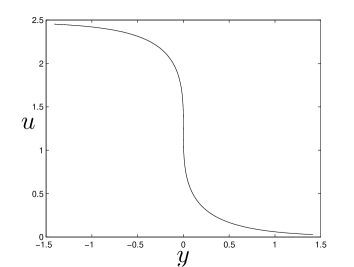
   (a) $\alpha=0.351648275547$

   

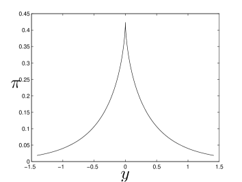
   (b) $\alpha=0.351648275547$

   

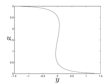
   (c) $\alpha=0.1$

   

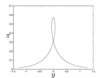
   (d) $\alpha=0.1$

   

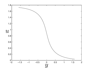
   (e) $\alpha=0.8$

   

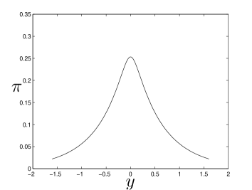
   (f) $\alpha=0.8$

   Figure 1: Shape $u$ and corresponding momentum $\pi$ of the soliton.

   $$4(k^{2}-\omega^{2})+2\alpha(k-\omega)-1=0,$$ (32)

   which may lead to the following solution ($k>0$)

   $$k=\frac{1}{\alpha(1-v)+\sqrt{\alpha^{2}(1-v)^{2}+4(1-v^{2})}},\quad\omega=kv,$$ (33)

   where $v$ is the velocity of the wave satisfying the condition $-1<v<1$. It seems worth noting here that from equations (21), (23) and (26), one may find that $y=-Z+C$, $C$ being an arbitrary constant. In order to discuss the soliton solutions to equation (19), it is important to consider the following relation

   $$\partial_{\sigma}=\frac{1}{2}\left[1-4(\omega+k)k\verb"sech"^{2}(\theta)\right]\partial_{Z}.$$ (34)

   We may pay interest to the shape of the soliton $u$ and its momentum $\pi=u_{\sigma}+u_{\tau}$. As a result, it comes that

   • for $\alpha=v\frac{\sqrt{1+v}}{1-v}$, $u_{Z}$ may never change sign but may be infinite at some ’singular’ point, whereas $\pi_{Z}$ may change sign once and may be infinite at the same singular point. Thus, $u$ may be monotone but may have an infinite derivative at this particular point, and $\pi$ may have a cusp-like shape (see panels 1(a) and 1(b));

   • for $\alpha\in\left[0,v\frac{\sqrt{1+v}}{1-v}\right[$, $u_{Z}$ may change sign twice and may be infinite at two singular points, whereas $\pi_{Z}$ may change sign three times. Thus, $u$ may follow a multi-valued shape with two singular points at their derivatives and $\pi$ may have a multi-valued profile especially a loop-like shape (see panels 1(c) and 1(d));

   • finally, for $\alpha\in\left]v\frac{\sqrt{1+v}}{1-v},\infty\right[$, $u_{Z}$ may never change sign and may never take infinite values. $\pi_{Z}$ may change sign once and may always be finite. Thus, $u$ may have a kink-like shape, whilst $\pi$ may have a single-valued profile especially a hump-like shape (see panels 1(e) and 1(f)).

   We give some illustrations of the previous discussions. Thus, we may take a velocity $v=0.24$ to plot the different profiles. The aforementioned shapes are clearly depicted in figure 1, at initial time $\tau=0$. Particularly, for the cusp-shape, the dissipative parameter is given by $\alpha=0.351648275547$.

In conclusion, the studies of the novel (1+1)-dimensional NLE equation (19) including the Vakhnenko and the variant SWSP equations (3) and (12), respectively, may have some scientific interests both from the viewpoint of the investigation of the propagation of high-frequency perturbations and from the viewpoint of the existence of stable wave formations. Thus, applications may be found in soliton theory, geodynamics, hydrodynamics and nonlinear optics, just to name a few.

References

References

- [1] Van D P B 1927 Phil. Mag. 3 65
- [2] Gukenheimer J and Holmes P J 1983 Nonlinear Oscillations, Dynamical Systems and Bifurcation of Vector Fields (Berlin: Springer-Verlag)
- [3] Ueda Y and Akamatsu 1981 IEEE Trans. 28 217
- [4] Kao Y H and Wang C S 1993 Phys. Rev.E 48 2514
- [5] Vakhnenko V O 1999 J. Math. Phys. 40 2011
- [6] Vakhnenko V O and Parkes E J 1998 Nonlinearity 11 1457
- [7] Vakhnenko V O, Parkes E J and Morrison A J 2003 Chaos Solitons Fractals 17 683
- [8] Morrison A J and Parkes E J 2001 Glasgow Math. J. 43 65
- [9] Morrison A J and Parkes E J 2003 Chaos Solitons Fractals 16 13
- [10] Nayfey A H 1973 Perturbation Methods (New-York: Wiley)
- [11] Nitropolsky Y A, Samoilenko A M and Martinyuk D I 1993 Systems of Evolution Equations With Periodic and Quasiperiodic Cfficients (Dordrecht: Kluwer Academic)
- [12] Fu Z, Liu S and Liu S 2007 J. Phys. A: Math. Gen. 40 4739
- [13] Schfer T and Wayne C E 2004 Physica D 196 90
- [14] Chung Y, Jones C K R T, Schfer T and Wayne C E 2006 Nonlinearity 18 1351
- [15] Sakovich A and Sakovich S 2005 J. Phys. Soc. Japan 74 239
- [16] Sakovich A and Sakovich S 2006 J. Phys. A: Math. Gen. 39 L361
- [17] Kuetche K V, Bouetou B T and Kofane T C 2007 J. Phys. Soc. Japan 76 024004
- [18] Kuetche K V, Bouetou B T and Kofane T C 2007 J. Phys. A: Math. Theor. 40 5585
- [19] Kuetche K V, Bouetou B T and Kofane T C 2007 J. Phys. Soc. Japan 76 073001
- [20] Parkes E J 2006 Chaos Solitons Fractals in press
- [21] Hirota R 1980 Solitons (New York: Springer)
- [22] Hirota R 1988 Direct Methods in Soliton Theory (Berlin: Springer-Verlag)
- [23] Kakuhata H and Konno K 1999 J. Phys. Soc. Japan 48 757