Drift Wave Model of Rotating Radio Transients

Abstract

During the last few years there were discovered and deeply examined several transient neutron stars ( Rotating Radio Transients ). It is already well accepted that these objects are rotating neutron stars. But their extraordinary features (burst-like behavior) made necessary revision of well accepted models of pulsar interior structure. Nowadays most popular model for RRATs is precessing pulsar model, which is the subject of big discussion. We assume that these objects are pulsars with specific spin parameters. An important feature of our model, naturally explaining most of the properties of these neutron stars, is presence of very low frequency, nearly transverse drift waves propagating across the magnetic field and encircling the open field lines region of the pulsar magnetosphere.

1 Introduction

Recently, McLaughlin et al. (2005) reported the discovery of a new class of radio transients from the Parkes Multibeam Pulsar Survey. The current sample includes 11 objects characterized by single, dispersed bursts of radio emission with the durations ranging from 2 to 30 milliseconds. Long-term monitoring of these objects led to identification of their spin periods (P), ranging from 0.4 to 7 seconds. As McLaughlin et al. (2005) concluded, these objects represent a previously unknown population of rotation-powered neutron stars, which were named as Rotating RAdio Transients (RRATs). Another interesting case between normal pulsars and RRATs have been reported earlier (PSRs J1649+2533 and J1752+2359) by Lewandowski et al. (2004). Understanding the physical origin of these objects as well as their relationship with normal pulsars is desirable. There exist few models for this phenomenon: 1) The precession model; 2) The model suggesting that these objects are pulsars located slightly below the radio emission death line , and become active occasionally when the conditions for pair production and coherent emission are satisfied; 3) The third model invoking a radio emission direction reversal in normal pulsars. In this picture, our line of sight misses the main radio emission beam of RRATs but happens to sweep the emission beam when the radio emission direction is reversed. Last two ideas were suggested by Zhang et al. (2006). Here we propose another model of RRATs proving once again that they are normal pulsars with special values of certain parameters.

The paper is organized as follows. Pulsar radio emission mechanism is presented in Section 2. The generation of the drift waves and their influence on the curvature of magnetic field lines are discussed in Section 3. Our proposed model is presented in Section 4. The conclusions are summarized in Section 5.

2 Emission mechanism

As it is known the pulsar magnetosphere is filled by a dense relativistic electron-positron plasma. The (e⁺e^-) pairs are generated as a consequence of the avalanche process (first described by Sturrock (1971)) and flow along the open magnetic field lines. The plasma is multi-component, with a one-dimensional distribution function ( see Fig.1 from Arons (1981)) and consists of the following components: the bulk of plasma with an average Lorentz-factor $\gamma_{p}\simeq 10$; a tail on the distribution function with $\gamma_{t}\simeq 10^{4}$ and the primary beam with $\gamma_{b}\simeq 10^{6}$. The main mechanism of wave generation in plasmas of the pulsar magnetosphere is the cyclotron instability. Generation of waves is possible if the condition of the cyclotron resonance if fulfilled (Kazbegi et al., 1991a):

$$\omega-k_{\varphi}V_{\varphi}-k_{x}u_{x}+\frac{\omega_{B}}{\gamma_{r}}=0,$$ (1)

where $V_{\varphi}$ is the particle velocity along the magnetic field, $\gamma_{r}$ is the Lorentz-factor for the resonant particles and $u_{x}=cV_{\varphi}\gamma_{r}/\rho\omega_{B}$ is the drift velocity of the particles due to curvature of the field lines ($\rho$ is the radius of curvature of the field lines and $\omega_{B}=eB/mc$ is the cyclotron frequency). Here cylindrical coordinate system is chosen, with the $x$-axis directed transversely to the plane of field line, when $r$ and $\varphi$ are the radial and azimuthal coordinates. Generated waves leave the magnetosphere propagating at very small angles to the pulsar local magnetic field lines and reach an observer as pulsar radio emission. These processes take place near the light cylinder where the cyclotron instability occurs (Lyutikov et al., 1999).

3 Change of field line curvature and emission direction by drift waves

It has been shown by Kazbegi et al. (1991b, 1996) that, in addition to the radio waves, very low frequency, nearly transverse drift waves can be excited in the same region. The period of the drift waves $P_{dr}$ can be written as:

$$P_{dr}=\frac{e}{4\pi^{2}mc}\frac{BP^{2}}{\gamma}$$ (2)

Where $P$ is the pulsar spin period, $B=B_{s}(R_{0}/R)^{3}$ is the magnetic field in the wave excitement region and $\gamma$ is the relativistic Lorentz factor of the particles. It appears that the period of the drift wave can vary in a broad range. The magnetic field of drift wave adds with pulsar magnetic field as $r$ component and causes changing of field line curvature $\rho_{c}$. Here and below the cylindrical coordinate system ($x,r,\varphi$) is chosen, with the $x$-axis directed transversely to the plane of field line, while $r$ and $\varphi$ are the radial and azimuthal coordinates, respectively.

Even a small change of $B_{r}$ causes significant change of $\rho_{c}$. Variation of the field line curvature can be estimated as

$$\frac{\Delta\rho}{\rho}\approx k_{\varphi}r\frac{\Delta B_{r}}{B_{\varphi}}$$ (3)

Here $k_{\varphi}$ is a longitudinal component of wave vector and $r$ is distance to the center of pulsar. It follows that even the drift wave with a modest amplitude $B_{r}\sim\Delta B_{r}\sim 0.01B_{\varphi}$ alters the field line curvature substantially, $\Delta\rho/\rho\sim 0.1$

Since radio waves propagates along the local magnetic field lines, curvature variation causes change of emission direction.

4 The model

There is unequivocal correspondence between the observable intensity and $\alpha$ (angle between observers line and emission direction (see fig. 1)). Maximum of intensity corresponds to minimum of $\alpha$. The period of pulsar is time interval between neighboring maxima of observable intensity i.e. minima of $\alpha$ (see fig. 2). According to this fact, we can say that the observable period depends on time behavior of $\alpha$ and as it will appear below it might differ from the spin period of pulsar.

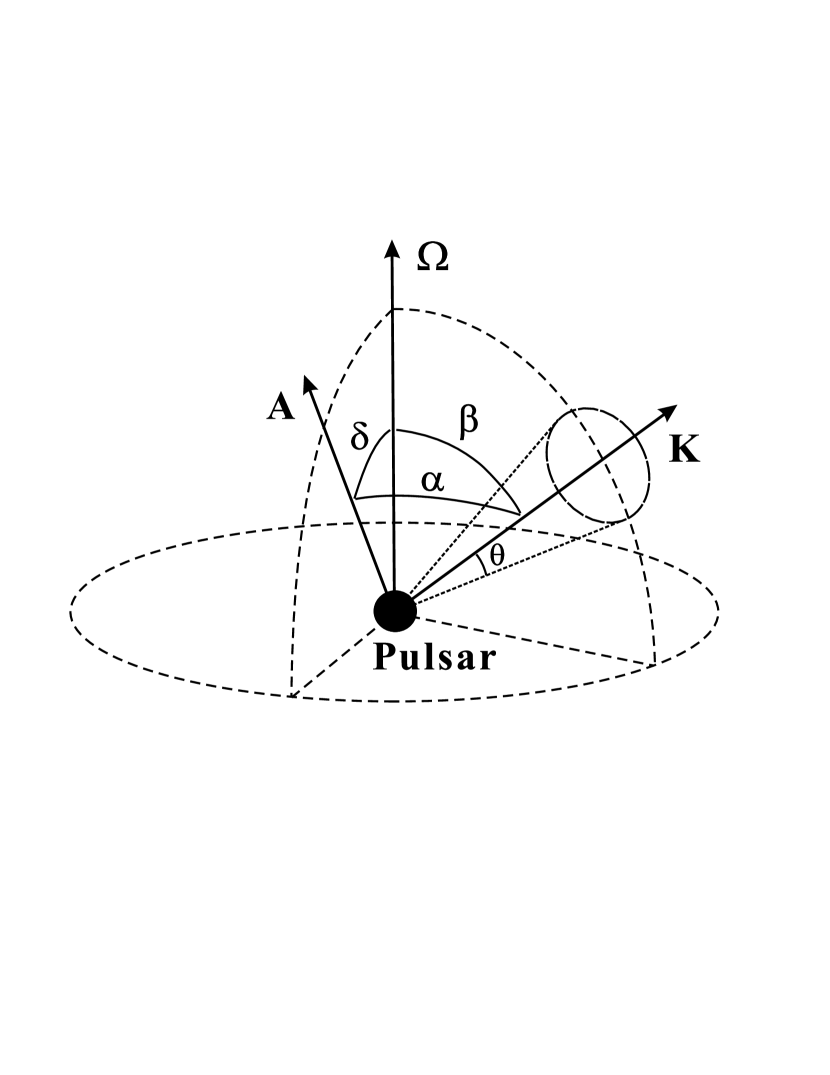
Figure 1: Geometry of $\Omega$ - rotation, K - emission and A - observers axes. Angles $\delta$ and $\vartheta$ are constants, while $\beta$ and $\alpha$ are oscillating with time.

$$\cos\alpha={\bf A}\cdot{\bf K}$$ (4)

${\bf A}$ and ${\bf K}$ are unit guide vectors of observers and emission axes respectively. In the spherical coordinate system ($r,\varphi,\theta$), combined with plane of pulsar rotation, these vectors can be expressed as:

$${\bf A}=\left(1,0,\delta\right)$$ (5)

$${\bf K}=\left(1,\Omega t,\beta\right)$$ (6)

where $\Omega=2\pi/P$ is the angular velocity of the pulsar. $\delta$ is the angle between rotation and observers axis, and $\beta$ is the angle between rotation and emission axis (see fig. 1). From equations (4),(5) and (6) follows that:

$$\alpha=\arccos\left(\sin\delta\sin\beta\cos\Omega t+\cos\delta\cos\beta\right)$$ (7)

In the absence of the drift wave $\beta=\beta_{0}=const$ and consequently the period of $\alpha$ equals to $2\pi/\Omega$, while in the case of existence of drift wave $\beta$ is oscillating with time (Lomiashvili et al., 2006).

Considering that for wavelengths of order of the transverse scale of magnetosphere, the treatment of the drift waves as plane waves becomes inappropriate the geometry of magnetosphere must be taken into account. A treatment in terms of spherical harmonic eigenmodes with specific $l,m$ is then appropriate (Gogoberidze et al., 2005). Therefore in general case the amplitude $\Delta\beta$ must be defined as follows

$$\Delta\beta=\sum\Delta\beta_{n}\sin\left(\omega^{n}_{dr}t+\varphi^{n}\right)$$ (8)

Here $n$ is number of eigenmode. According to equations (7) and (8) we obtain

$$\alpha=\arccos[\sin\delta\sin\left(\beta_{0}+\sum\Delta\beta_{n}\sin\left(\omega^{n}_{dr}t+\varphi^{n}\right)\right)\cos\Omega t$$

$$+\cos\delta\cos\left(\beta_{0}+\sum\Delta\beta_{n}\sin\left(\omega^{n}_{dr}t+\varphi^{n}\right)\right)]$$ (9)

$$\alpha_{\min}^{k}=\left|\left(\beta_{0}-\delta\right)+\Delta\beta\sin\left(2\pi k\frac{\omega_{dr}}{\Omega}+\varphi\right)\right|$$ (10)

Where $\alpha_{\min}^{k}$ is the minimum of $\alpha$ after $k$ revolutions of the pulsar, after time reckoning. The parameters of the pulse profile (e.g. width, height etc.) significantly depend on what the minimal angle would be between emission axis and observers axis when the first one passes the other (during one revolution). If the emission cone does not cross the observers line of sight entirely (i.e. minimal angle between them is more then cone angle $\vartheta$, see inequality (11)) then pulsar emission is unobservable for us. On the other hand, inequality (12) defines condition that is necessary for emission detection.

$$\alpha_{\min}^{k}>\vartheta$$ (11)

$$\alpha_{\min}^{k}<\vartheta$$ (12)

Hence for some values of parameters $\Omega$, $\omega_{dr}$, $\beta$, $\Delta\beta$, $\delta$, $\varphi$ and $\vartheta$ (Set A) it is possible to accomplish following regime: Once condition (12) becomes fulfilled it stays along $k$ revolutions, therefore pulsar is observable during $k$ periods. While over the the other $m-k$ revolutions condition (11) accomplishes, consequently pulsar appears ”switched off” (see Fig. 2). It means that burst-like emission occurs.

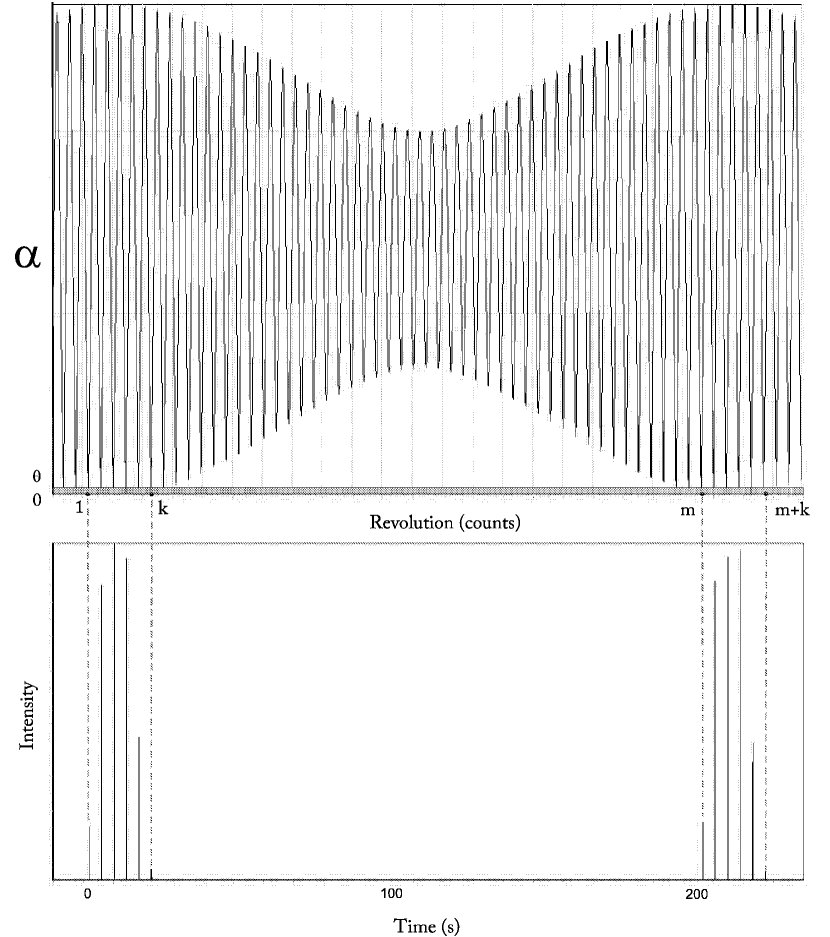
Figure 2: The oscillating behavior of $\alpha$ with time  for $\beta_{0}=1.35$, $\delta=1.0$, $\Delta\beta=0.35$, $\omega_{dr}=2\pi(1/4.26+1/204.4)(s^{-1})$, $\Omega=2\pi/4.26(s^{-1})$, $\varphi=1.5$ and Simulated lightcurve of PSR J1819-1458

(below)

PSR J1752+2359 has been selected for its unusually long nulling periods. It had been observed on several occasions between 2000 and 2002 by Lewandowski et al. (2004). The pulsar spends 70- 80% of the time in a quasi-null state. The on-states occur once every 400-600 periods and last, on average, for $\sim 100$ periods. A more detailed inspection of the on-states reveals that these burst-like emissions are quite similar in shape and duration and they decay into a null state in a manner that is quite reasonably described by a $te^{-t/\tau}$ function with $\tau\sim 45$ seconds. PSR J1752+2359 switches off gradually, rather than suddenly. Simulated lightcurve of J1752+2359 is presented in Fig. 3.

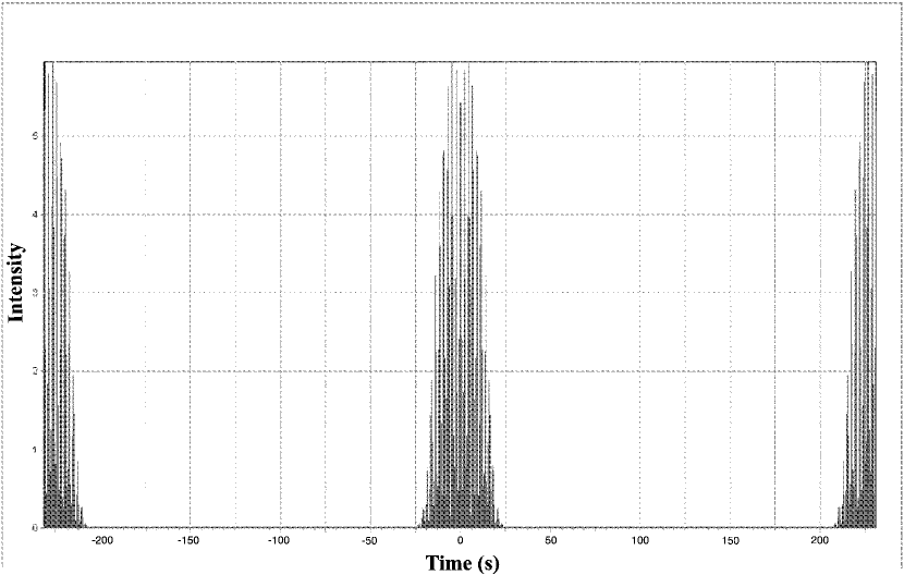
Figure 3: Simulated lightcurve of PSR J1752+2359

If we consider these pulsars in the framework of our model their parameters (spin, angular etc.) will get values shown in Table 1. Simulated lightcurve of PSR J1819-1458 (RRAT J1819-1458) is presented in Fig. 2.

5 Conclusions

To sum up, drift wave driven model is very convenient since it allows to explain almost every extraordinary feature of known pulsars such as: extremely long periods (Lomiashvili et al., 2006), cyclic variations of radiation intensity (RRATs) and rotational parameters (in prep.), subpulse drift (Gogoberidze et al., 2005), nullings (Kazbegi et al., 1996), etc. Moreover it has potentiality to unfold future discoveries in this field.

In long period radio pulsars (Lomiashvili et al., 2006) relation between periods of pulsar and drift wave along with pulsar geometry satisfy much precise condition than in RRATs. Therefore total number of RRATs should be much more than long period radio pulsars.

The precession model is very similar to ours although it has number of disadvantages. First of all, it is necessary to take large value of wobble angle to interpret observational data of some RRATs. In the case of neutron stars this is hard to explain because of their superfluid interior structure. However, there is a need of distinguishable sign to elucidate which model is true. Zhang et al. (2006) reported that one of the such tests would be search of X-ray counterpart from RRATs. Particularly, presence of a hot-spot thermal component in the possible X-ray spectra will mean that the emission direction reversal and a preferred viewing geometry are likely the agents to make a RRAT. While absence of X-ray radiation indicates that considering pulsars are ”not-quite-dead pulsars before disappearing in the graveyard.”

We suggest to investigate the power spectrum of the single-pulse observational data thoroughly. In our opinion, the power spectrum should be composition of few slightly broadened areas (ranges with peaks) instead of thin lines. Finding this kind of signature in the power spectra of RRATs will help to asses wether the origin of the transient nature of these objects is indeed plasmic, as suggested by our model.

Table 1: The values of pulsar parameters

PSR	$P$	$\Delta\beta$	$\beta_{0}$	$\delta$	$\vartheta$
J1752+2359	0.41	0.2	1.2	1	0.03
J1819-1458	4.26	0.35	1.35	1	0.03

References

- Arons (1981) Arons J., 1981a, Plasma Astrophys., 273
- Gogoberidze et al. (2005) Gogoberidze, G., Machabeli, G.Z., Melrose, D.B., & Luo, Q. 2005, MNRAS, 360, 669
- Kazbegi et al. (1991a) Kazbegi A. Z., Machabeli G. Z., Melikidze G. I., Smirnova T. V., 1991a, Afz, 34, 433
- Kazbegi et al. (1991b) Kazbegi A. Z., Machabeli G. Z., Melikidze G. I., 1991b, MNRAS, 253, 377
- Kazbegi et al. (1996) Kazbegi A. Z., Machabeli G. Z., Melikidze G. I., Shukre C., 1996, A&A, 309, 515
- Lewandowski et al. (2004) Lewandowski W., Wolszczan A., Feiler G., Konacki M., & Soltysinski T., 2004, ApJ, 600, 905
- Lomiashvili et al. (2006) Lomiashvili D., Machabeli G., & Malov I., 2006, ApJ, 637, 1010
- Lyutikov et al. (1999) Lyutikov M, Blandford R., Machabeli G., 1999, MNRAS, 305, 338L
- McLaughlin et al. (2005) McLaughlin M. A., Lyne A. G., Lorimer D. R., Kramer M., Faulkner A. J., Manchester R. N., Cordes J. M., Camilo F., Possenti A., Stairs I. H., Hobbs G., D Amico N., Burgay M., & O Brien J. T., 2005, (astro-ph/0511587)
- Sturrock (1971) Sturrock P. A., 1971, ApJ, 164, 529
- Zhang et al. (2006) Zhang B., Gil J., & Dyks J., 2006, (astro-ph/0601063)