Closed trajectories of a particle model
on null curves in anti-de Sitter 3-space

Abstract.

We study the existence of closed trajectories of a particle model on null curves in anti-de Sitter 3-space defined by a functional which is linear in the curvature of the particle path. Explicit expressions for the trajectories are found and the existence of infinitely many closed trajectories is proved.

1. Introduction

In this paper we study null curves in anti-de Sitter 3-space which are critical points for the functional

(1) $$\mathcal{L}(\gamma)=\int_{\gamma}{(m+k_{\gamma})}ds,\quad m\in\mathbb{R},$$

where $s$ is the pseudo-arc parameter which normalizes the derivative of the tangent vector field of $\gamma$ and $k_{\gamma}(s)$ is a curvature function that, in general, uniquely determines $\gamma$ up to Lorentz transformations ([4], [9]). The functional (1) is invariant under the group $\mathrm{SL}(2,\mathbb{R})\times\mathrm{SL}(2,\mathbb{R})$, which doubly covers the identity component of the group of Lorentz transformations. Motivations for this study are provided by optimal control theory and especially by the recent interest in certain particle models on null curves in Lorentzian 3-space forms associated with action integrals of the type above ([11], [4]). Yet another motivation is given by surface geometry; if we take $\mathrm{SL}(2,\mathbb{R})$ as a model for anti-de Sitter 3-space, then a null curve in anti-de Sitter 3-space, as real form of a holomorphic null curve in $\mathrm{SL}(2,\mathbb{C})$, is related to the theory of constant mean curvature one (cmc-1) surfaces and flat fronts in hyperbolic 3-space ([2], [13], [5]). In perspective, one would like to understand the class of cmc-1 surfaces generated by the critical points of (1).

The purpose of this article is to investigate the global behavior of extremal trajectories of the functional (1). We will find explicit expressions for the extremal trajectories and then establish the existence of infinitely many closed ones. This result is related to the presence of maximal compact abelian subgroups in the isometry group $\mathrm{SL}(2,\mathbb{R})\times\mathrm{SL}(2,\mathbb{R})$ of anti-de Sitter 3-space. For a discussion of extremal trajectories in the other Lorentzian space forms we refer to [6], [10].

The Euler–Lagrange equation associated to (1) yields that the curvature of extremal trajectories is either a constant, in which case we have null helices, or an elliptic function of the pseudo-arc parameter. In this case, extremal trajectories are governed by a second order linear ODE with doubly periodic coefficients. By classical results of Picard [12] in the Fuchsian theory of linear ODEs, the solution curves are then expressible in terms of the Weierstrass $\wp$, $\sigma$ and $\zeta$ functions (cf. Theorem 1). The explicit integration of extremal trajectories amounts to the integration of a linearizable flow on $K_{1}\times K_{2}$, where $K_{1}$ and $K_{2}$ are 1-dimensional abelian subgroups of $\mathrm{SL}(2,\mathbb{R})$. In particular, if $K_{1}=K_{2}=\mathrm{SO}(2)$, the integration amounts to solving a linearizable first-order ODE on a 2-dimensional torus. This setting strongly suggests the possibility of periodic solutions. That this is indeed the case is established in Theorem 2 where the existence of countably many periodic trajectories is proved by studying the map of periods. The proof relies on computations made with Mathematica.

The paper is organized as follows. Section 2 contains some background material. Section 3 provides the explicit integration of extremal trajectories. Section 4 discusses periodic trajectories and proves the existence of infinitely many of them. The Appendix outlines the derivation of the Euler-Lagrange equation associated with (1) via the Griffiths formalism [7].

2. Preliminaries

Anti-de Sitter 3-space, $\mathbb{H}^{3}_{1}$, can be viewed as the special linear group $\mathrm{SL}(2,\mathbb{R})$ endowed with the bi-invariant Lorentz metric of constant sectional curvature $-1$ defined by the quadratic form

(2) $$q(X)=(x^{1}_{1})^{2}+x^{1}_{2}x^{2}_{1}=-\mathrm{det\,}X,$$

for each $X=(x^{i}_{j})\in\mathfrak{sl}(2,\mathbb{R})$. The group $G=\mathrm{SL}(2,\mathbb{R})\times\mathrm{SL}(2,\mathbb{R})$ acts transitively by isometries on $\mathbb{H}^{3}_{1}\cong\mathrm{SL}(2,\mathbb{R})$ via the action

$$(A,B)\cdot x=AxB^{-1}.$$

The stability subgroup at the identity $I_{2}$ is the diagonal group

$$\Delta=\{(A,A)\,|\,A\in\mathrm{SL}(2,\mathbb{R})\}$$

and $\mathbb{H}^{3}_{1}$ may be described as a Lorentzian symmetric space

$$\mathbb{H}^{3}_{1}\cong G/\Delta.$$

The projection

$$\pi:G\ni(A,B)\mapsto AB^{-1}\in\mathrm{SL}(2,\mathbb{R})$$

makes $G$ into a principal bundle with structure group $\Delta$.

Let $I\subset\mathbb{R}$ be any open interval of real numbers. A smooth parametrized curve $\gamma:I\to\mathrm{SL}(2,\mathbb{R})$ is null, or lightlike, if $\mathrm{det\,}(\gamma^{-1}\gamma^{\prime})$ vanishes identically. If $\gamma$ has no flex points, there exists a canonical lift

$$\Gamma=(\Gamma_{+},\Gamma_{-}):I\to G$$

such that

(3) $$\Gamma_{+}^{-1}d\Gamma_{+}=\left(\begin{array}[]{cc}0&1\\ k+1&0\\ \end{array}\right)\omega,\quad\Gamma_{-}^{-1}d\Gamma_{-}=\left(\begin{array}[]{cc}0&1\\ k-1&0\\ \end{array}\right)\omega,$$

where $\omega$ is a nowhere vanishing 1-form, the canonical arc element, and $k:I\to\mathbb{R}$ is a smooth function, the curvature function. We call $\Gamma$ the spinor frame field along $\gamma$ and its components $\Gamma_{+}$ and $\Gamma_{-}$ the positive and negative spinor frame, respectively. The spinor frame $\Gamma$ is essentially unique, in the sense that $\pm\Gamma$ are the only lifts satisfying (3). Throughout the paper we will consider null curves without flex points and parametrized by the natural parameter, i.e., $\omega=ds$ (cf. [4], [3]).

Conversely, for a smooth function $k:I\to\mathbb{R}$, let $H_{\pm}(k):I\to\mathfrak{sl}(2,\mathbb{R})$ be

(4) $$H_{+}(k)=\left(\begin{array}[]{cc}0&1\\ k+1&0\\ \end{array}\right),\quad H_{-}(k)=\left(\begin{array}[]{cc}0&1\\ k-1&0\\ \end{array}\right).$$

By solving a linear system of ODEs, there exists a unique (up to left multiplication)

$$\Gamma=(\Gamma_{+},\Gamma_{-}):I\to G$$

such that

$$\Gamma_{+}^{-1}{\Gamma}^{\prime}_{+}=H_{+}(k),\quad\Gamma_{-}^{-1}{\Gamma}^{\prime}_{-}=H_{-}(k).$$

In particular, $\gamma=\Gamma_{+}\Gamma_{-}^{-1}:I\to\mathrm{SL}(2,\mathbb{R})$ is a null curve without flex points, parametrized by the natural parameter and with curvature function $k$.

In this context, two null curves $\gamma:I\to\mathrm{SL}(2,\mathbb{R})$, $\tilde{\gamma}:\tilde{I}\to\mathrm{SL}(2,\mathbb{R})$ are said equivalent if there exist $c\in\mathbb{R}$ and $A,B\in\mathrm{SL}(2,\mathbb{R})$ such that $\tilde{\gamma}(s)=A\gamma(s+c)B^{-1}$, for all $s\in\tilde{I}$.

Definition. An extremal trajectory (or simply, a trajectory) in $\mathbb{H}^{3}_{1}$ is a null curve with non-constat curvature which is a critical point of the action functional

(5) $$\mathcal{L}_{m}(\gamma)=\int_{\gamma}{(m+k_{\gamma})\omega}$$

under compactly supported variations, where the Lagrange multiplier $m$ is a real constant.

The Euler-Lagrange equation associated to $\mathcal{L}_{m}$ is computed to be

$${k}^{\prime\prime\prime}-6k{k}^{\prime}+2m{k}^{\prime}=0$$

(cf. [4]; see also the Appendix for a different way of deriving this equation). This may be thought of as the intrinsic equation of a trajectory. If we let $h:=\frac{1}{2}(k-\frac{m}{3})$ be the reduced curvature, then $h$ satisfies

(6) $$({h}^{\prime})^{2}=4h^{3}-g_{2}h-g_{3},$$

for real constants $g_{2}$ and $g_{3}$. Hence $h$ is expressed by the real values of either a Weierstrass $\wp$-function with invariants $g_{2}$, $g_{3}$, or one of its degenerate forms.

We call a solution to (6) a potential with analytic invariants $g_{2}$, $g_{3}$. Two potentials are considered equivalent if they differ by a reparametrization of the form $s\mapsto s+c$, where $c$ is a constant. For real $g_{2}$ and $g_{3}$, let $\Delta(g_{2},g_{3})=27g_{3}^{2}-g_{2}^{3}$ be the discriminant of the cubic polynomial

$$P(t;g_{2},g_{3})=4t^{3}-g_{2}t-g_{3}.$$

The study of the real values of the Weierstrass $\wp$-function with real invariants $g_{2}$, $g_{3}$ (and its degenerate forms) leads to primitive half-periods $\omega_{1}$, $\omega_{3}$ such that:

• $\Delta(g_{2},g_{3})<0$: $\omega_{1}>0$, $\omega_{3}=i\nu\omega_{1}$, $\nu>0$.

• $\Delta(g_{2},g_{3})>0$: $\omega_{1}>0$, $\omega_{3}=\frac{1}{2}(1+i\nu)\omega_{1}$, $\nu>0$.

• $\Delta(g_{2},g_{3})=0$ and $g_{3}>0$: $\omega_{1}>0$, $\omega_{3}=+i\infty$.

• $\Delta(g_{2},g_{3})=0$ and $g_{3}<0$: $\omega_{1}=+\infty$, $-i\omega_{3}>0$.

• $g_{2}=g_{3}=0$: $\omega_{1}=+\infty$, $\omega_{3}=+i\infty$.

Accordingly, denoting by $\mathcal{D}(g_{2},g_{3})$ the fundamental period-parallelogram spanned by $2\omega_{1}$ and $2\omega_{3}$, the only possible cases for the potential function $h:I\to\mathbb{R}$ are:

• $\Delta<0$: $h(s)=\wp(s;g_{2},g_{3})$, $I=(0,2\omega_{1})$.

• $\Delta<0$: $h(s)=\wp_{3}(s;g_{2},g_{3})=\wp(s+\omega_{3};g_{2},g_{3})$, $I=\mathbb{R}$.

• $\Delta>0$: $h(s)=\wp(s;g_{2},g_{3})$, $I=(0,2\omega_{1})$.

• $\Delta=0$, $g_{3}=-8a^{3}>0$:

  $$h(s)=-3a\tan^{2}{\left({\sqrt{-3a}}{s}\right)}-2a,\quad I=(-\frac{\pi}{\sqrt{-12a}},\frac{\pi}{\sqrt{-12a}}).$$

• $\Delta=0$, $g_{3}=-8a^{3}<0$:

  $$h(s)=3a\tanh^{2}{\left({\sqrt{3a}}{s}\right)}-2a,\quad I=\mathbb{R}.$$

• $g_{2}=g_{3}=0$: $h(s)={s^{-2}}$, $I=(-\infty,0)$ or $I=(0,+\infty)$.

3. Integration of the extremal trajectories

For a potential function $h$ with invariants $g_{2}$, $g_{3}$, let

$$\mu_{\pm}(m,h):=\frac{1}{2}\sqrt{P\left(\frac{m}{3}\pm 1;g_{2},g_{3}\right)},$$

and, for each $s_{0}\in I$, define $\phi_{\pm}(m,h,s_{0}):I\to\mathbb{R}$ by

$$\phi_{\pm}(m,h,s_{0})=\begin{cases}\displaystyle\int_{s_{0}}^{s}{\frac{\mu_{\pm}(m,h)}{h(u)-\left(\frac{m}{3}\pm 1\right)}du},\quad\mu_{\pm}(m,h)\neq 0,\\ \displaystyle\int_{s_{0}}^{s}{\frac{1}{h(u)-\left(\frac{m}{3}\pm 1\right)}du},\quad\mu_{\pm}(m,h)=0.\end{cases}$$

Next, let $w_{\pm}(m,h)$ be the unique points in $\mathcal{D}(g_{2},g_{3})$ such that

$$h(w_{\pm})=\frac{m}{3}\pm 1\quad\text{and}\quad h^{\prime}(w_{\pm})=2\mu_{\pm}(m,h).$$

Then, denoting by $\sigma_{h}$ and $\zeta_{h}$, respectively, the sigma and zeta Weierstrassian functions corresponding to the potential $h$, we compute:

Case I: if $\mu_{\pm}(m,h)\neq 0$,

$$\phi_{\pm}(m,h,s_{0})=\log{\frac{\sigma_{h}(s-w_{\pm})}{\sigma_{h}(s+w_{\pm})}}+2s\zeta_{h}(w_{\pm})+c(s_{0}).$$

Case II: if $\mu_{\pm}(m,h)=0$ and $g_{2}^{2}+g_{3}^{2}\neq 0$,

$$\phi_{\pm}(m,h,s_{0})=\frac{-1}{3\left(\frac{m}{3}\pm 1\right)^{2}-g_{2}/4}\left\{\zeta_{h}(s+w_{\pm})+\left(\frac{m}{3}\pm 1\right)s\right\}+c(s_{0}).$$

Case III: if $\mu_{\pm}(m,h)=0$ and $g_{2}=g_{3}=0$,

$$\phi_{\pm}(m,h,s_{0})=\frac{1}{3}s^{3}+c(s_{0}).$$

Accordingly, define the maps $R_{\pm}(m,h)$, $D_{\pm}(m,h,s_{0}):I\to\mathrm{GL}(2,\mathbb{C})$ as follows:

Case I: if $\mu_{\pm}(m,h)\neq 0$,

$$R_{\pm}(m.h)=\displaystyle\frac{1}{{2\mu_{\pm}}}\left(\begin{array}[]{cc}-\displaystyle\frac{{h^{\prime}}-2\mu_{\pm}(m,h)}{2\sqrt{h-\left(\frac{m}{3}\pm 1\right)}}&-\sqrt{h-\left(\frac{m}{3}\pm 1\right)}\\ \displaystyle\frac{{h^{\prime}}+2\mu_{\pm}(m,h)}{2\sqrt{h-\left(\frac{m}{3}\pm 1\right)}}&\sqrt{h-\left(\frac{m}{3}\pm 1\right)}\\ \end{array}\right),$$

$$D_{\pm}(m,h,s_{0})=\left(\begin{array}[]{cc}\displaystyle\exp{(-\phi_{\pm}(m,h,s_{0}))}&\displaystyle 0\\ \displaystyle 0&\displaystyle\exp{(\phi_{\pm}(m,h,s_{0}))}\\ \end{array}\right).$$

Case II: if $\mu_{\pm}(m,h)=0$,

$$R_{\pm}(m.h)=\left(\begin{array}[]{cc}\displaystyle 1&0\\ \displaystyle\frac{{h^{\prime}}}{2\sqrt{h-\left(\frac{m}{3}\pm 1\right)}}&\sqrt{h-\left(\frac{m}{3}\pm 1\right)}\\ \end{array}\right),$$

$$D_{\pm}(m,h,s_{0})=\left(\begin{array}[]{cc}\displaystyle\frac{1}{\sqrt{h-(\frac{m}{3}\pm 1)}}&\displaystyle\phi_{\pm}(m,h,s_{0})\\ \displaystyle 0&\displaystyle 1\\ \end{array}\right).$$

Finally, define the maps $\Gamma_{\pm}(m,h,s_{0})$, $\gamma(m,h,s_{0}):I\to\mathrm{GL}(2,\mathbb{C})$ by

$$\Gamma_{\pm}(m,h,s_{0}):=R_{\pm}(m,h)(s_{0})^{-1}D_{\pm}(m,h,s_{0})(s_{0})^{-1}D_{\pm}(m,h,s_{0})R_{\pm}(m,h),$$

$$\gamma(m,h,s_{0}):=\Gamma_{+}(m,h,s_{0})\,\Gamma_{-}(m,h,s_{0})^{-1}.$$

We are now in a position to state the following.

Theorem 1.

The curve $\gamma(m,h,s_{0})$ takes values in $\mathbb{H}^{3}_{1}\cong\mathrm{SL}(2,\mathbb{R})$ and defines an extremal trajectory with multiplier $m$ and reduced curvature $h$. In particular, any extremal trajectory is equivalent to a curve of this type.

Proof.

A direct, lengthy computation shows that

(7) $$\Gamma_{\pm}(m,h,s_{0})^{-1}\,\Gamma_{\pm}(m,h,s_{0})^{\prime}=H(m,h)_{\pm},$$

where

(8) $$H_{+}(m,h)=\left(\begin{array}[]{cc}0&1\\ 2h+\frac{m}{3}+1&0\\ \end{array}\right),\quad H_{-}(m,h)=\left(\begin{array}[]{cc}0&1\\ 2h+\frac{m}{3}-1&0\\ \end{array}\right).$$

Equations (7) and (8) imply that $\Gamma_{\pm}(m,h,s_{0})$ take values in a left coset of $\mathrm{SL}(2,\mathbb{R})$. Our normalization implies that $\Gamma_{\pm}(m,h,s_{0})(s_{0})=I_{2}$, and hence that $\Gamma_{\pm}(m,h,s_{0})$ and $\gamma(m,h,s_{0})$ take values in $\mathrm{SL}(2,\mathbb{R})$. On the other hand, (7) and (8) imply that $\Gamma(m,h,s_{0})=\left(\Gamma_{+}(m,h,s_{0}),\Gamma_{-}(m,h,s_{0})\right)$ is a spinor frame field with multiplier $m$ and curvature function $k=2h+\frac{m}{3}$. Therefore, $\gamma(m,h,s_{0})$ is a trajectory with curvature function $k$. This proves the required result. ∎

4. Periodic trajectories

A trajectory is said quasi-periodic if its reduced curvature is a periodic function and if $\mu_{\pm}(m,h)$ are purely imaginary. Let $Q\left(t;\ell,e_{1}\right)$ be the cubic polynomial

$$Q\left(t;\ell,e_{1}\right)=4t^{3}-12\frac{(\ell^{4}-\ell^{2}+1)e_{1}}{(2-\ell^{2})^{2}}t+4\frac{(2\ell^{4}+\ell^{2}-1)e^{3}_{1}}{(2-\ell^{2})^{2}}.$$

The reduced curvature of a quasi-periodic trajectory can be written in the form

(9) $$h(s;\ell,e_{1})=e_{1}\left(\frac{3\ell^{2}}{2-\ell^{2}}\mathrm{sn}^{2}\left(\sqrt{\frac{3e_{1}}{2-\ell^{2}}}s,\ell\right)-\frac{1+\ell^{2}}{2-\ell^{2}}\right),$$

where $(m,\ell,e_{1})$ belongs to

$$\mathcal{W}=\{(m,\ell,e_{1})\in\mathbb{R}^{3}\,|\,e_{1}>0,\,\ell\in(0,1),\,Q\left(\frac{m}{3}\pm 1;l,e_{1}\right)<0\}.$$

The period of $h(s;\ell,e_{1})$ is given by

$$p(\ell,e_{1})=2\sqrt{\frac{2-\ell^{2}}{3e_{1}}}K(\ell),$$

where $K$ is the complete elliptic integral of the third kind. We put

$$\rho_{\pm}(m,\ell,e_{1})=\frac{1}{2}\sqrt{-Q\left(\frac{m}{3}\pm 1;\ell,e_{1}\right)}$$

and let $\mathcal{P}=(\mathcal{P}_{+},\mathcal{P}_{-}):\mathbb{R}\times\mathcal{W}\to\mathbb{R}^{2}$ be the analytic map

$$\mathcal{P}_{\pm}(s,m,\ell,e_{1})=\displaystyle\int_{0}^{1}{\frac{\rho_{\pm}(m,\ell,e_{1})}{h(u;m,\ell,e_{1})-\left(\frac{m}{3}\pm 1\right)}}du.$$

Recall that the spinor frame fields of $h$ are of the form

$$\Gamma_{\pm}(s)=C\cdot\left(\begin{array}[]{cc}\displaystyle\exp{(i\mathcal{P}_{\pm}(s,m,\ell,e_{1}))}&\displaystyle 0\\ \displaystyle 0&\displaystyle\exp{(-i\mathcal{P}_{\pm}(s,m,\ell,e_{1}))}\\ \end{array}\right)\cdot M(s),$$

where $C\in\mathrm{GL}(2,\mathbb{C})$ and $M:\mathbb{R}\to\mathrm{GL}(2,\mathbb{C})$ is a periodic map with period $p(\ell,e_{1})$. If we set $\Pi(m,\ell,e_{1})=\mathcal{P}(p(\ell,e_{1}),m,\ell,e_{1})$, for each $(m,\ell,e_{1})\in\mathcal{W}$, then a quasi-periodic trajectory with invariants $(m,\ell,e_{1})\in\mathcal{W}$ is periodic if and only if $\Pi(m,\ell,e_{1})\in\mathbb{Q}\times\mathbb{Q}$.

We can state the following.

Theorem 2.

There exists a discrete subset $\mathcal{M}_{0}\subset\mathbb{R}$ such that, for every $m\in\mathbb{R}\setminus\mathcal{M}_{0}$, there exist countably many periodic trajectories with multiplier $m$.

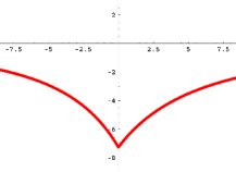
Figure 1. The graph of the function $f$.

Proof.

Consider the analytic map

$$\Psi:\mathcal{W}\ni(m,\ell,e_{1})\mapsto\frac{\partial(\Pi_{+},\Pi_{-})}{\partial(\ell,e_{1})}|_{(m,\ell,e_{1})}\in\mathbb{R}.$$

If $\Psi(m,\tilde{\ell},\tilde{e_{1}})\neq 0$, then $\Pi_{m}:(\ell,e_{1})\to\Pi(m,\ell,e_{1})\in\mathbb{R}^{2}$ is a local diffeomorphism near $(\tilde{\ell},\tilde{e_{1}})$. In this case there exist countably many closed trajectories with multiplier $m$. The mapping $\Psi$ can be computed explicitly, or numerically. To avoid dealing with quite long formulae, we would rather adopt the numerical viewpoint. Once we know $\Psi$, we define $f:\mathbb{R}\to\mathbb{R}$, $m\mapsto 400\Psi(m,\frac{1}{4},|m|+10)$. This is an analytic function for $m<0$ and for $m>0$. Looking at the graph of $f$ (cf. Figure 1), we see that $f\neq\text{const.}$ This implies that the set $\mathcal{M}_{0}=\{m\in\mathbb{R}\,|\,f(m)=0\}$ is a discrete set and that, for every $m\in\mathbb{R}\setminus\mathcal{M}_{0}$, there exist countably many closed trajectories with multiplier $m$. ∎

5. Appendix: Derivation of the Euler–Lagrange equation

In this section, we outline the derivation of the Euler-Lagrange equation associated with the $G$-invariant functional (1). We follow a general construction for invariant variational problems with one independent variable (due to Griffiths) and write the Euler–Lagrange equation as a Pfaffian differential system (PDF) $(\mathcal{J},\omega)$ on an associated manifold $Y$. We adhere to the terminology and notations used in [7].

5.1. The variational problem

The starting point of the construction is the replacement of the original variational problem on null curves in $\mathrm{SL}(2,\mathbb{R})$ by a $G$-invariant variational problem for integral curves of a Pfaffian differential system (PDF) with an independence condition on $M:=G\times\mathbb{R}$.

Let $(\alpha,\beta)$ be the Maurer–Cartan form of $G=\mathrm{SL}(2,\mathbb{R})\times\mathrm{SL}(2,\mathbb{R})$, where

(10) $$\alpha=\left(\begin{array}[]{cc}\alpha^{1}_{1}&\alpha^{1}_{2}\\ \alpha^{2}_{1}&-\alpha^{1}_{1}\\ \end{array}\right),\quad\beta=\left(\begin{array}[]{cc}\beta^{1}_{1}&\beta^{1}_{2}\\ \beta^{2}_{1}&-\beta^{1}_{1}\\ \end{array}\right).$$

The Maurer-Cartan equations of $G$, or the structure equations, are given by

$$\begin{cases}d\alpha^{1}_{1}=-\alpha^{1}_{2}\wedge\alpha^{2}_{1}\\ d\alpha^{2}_{1}=2\alpha^{1}_{1}\wedge\alpha^{2}_{1}\\ d\alpha^{1}_{2}=-2\alpha^{1}_{1}\wedge\alpha^{1}_{2}\end{cases}\quad\begin{cases}d\beta^{1}_{1}=-\beta^{1}_{2}\wedge\alpha^{2}_{1}\\ d\beta^{2}_{1}=2\beta^{1}_{1}\wedge\alpha^{2}_{1}\\ d\beta^{1}_{2}=-2\beta^{1}_{1}\wedge\alpha^{1}_{2}.\end{cases}$$

On $M:=G\times\mathbb{R}$, consider the PDS $(\mathcal{I},\omega)$ defined by the differential ideal $\mathcal{I}$ generated by the linearly independent 1-forms

$$\begin{cases}\eta^{1}=\frac{1}{2}(\alpha^{1}_{2}-\beta^{1}_{2}),\quad\eta^{2}=\alpha^{1}_{1},\quad\eta^{3}=\beta^{1}_{1},\\ \eta^{4}=\frac{1}{2}(\alpha^{1}_{2}+\beta^{1}_{2})-\omega,\quad\eta^{5}=\frac{1}{2}(\alpha^{2}_{1}+\beta^{2}_{1})-k\omega,\end{cases}$$

where

$$\omega:=\frac{1}{2}(\alpha^{2}_{1}-\beta^{2}_{1})$$

gives the independence condition $\omega\neq 0$. Now, if $\gamma:I\to\mathrm{SL}(2,\mathbb{R})$ is a null curve without flex points, then the curve $(\Gamma_{\gamma};k_{\gamma}):I\to M$, whose components are, respectively, the spinor frame field $\Gamma=(\Gamma_{+},\Gamma_{-})$ along $\gamma$ and the curvature of $\gamma$, is an integral curve of $(\mathcal{I},\omega)$ (cf. Section 2). Conversely, any integral curve $(\Gamma,k):I\to M$ of $(\mathcal{I},\omega)$ defines a null curve with no flex points $\gamma:I\to\mathrm{SL}(2,\mathbb{R})$, where $\Gamma$ is the spinor field along $\gamma$, and $k$ is the curvature of $\gamma$. So, null curves without flex points in $\mathrm{SL}(2,\mathbb{R})$ are identified with the integral curves of $(\mathcal{I},\omega)$.

From the above discussion, it follows that a null curve $\gamma$ without flex points is an extremal trajectory if and only if the pair $(\Gamma_{\gamma},k_{\gamma})$ of its spinor frame field $\Gamma_{\gamma}$ and curvature $k_{\gamma}$ is a critical point of the functional defined on the space $\mathcal{V}(\mathcal{I},\omega)$ of integral curves of $(\mathcal{I},\omega)$ by

(11) $$\widehat{\mathcal{L}}:(\Gamma,k)\in\mathcal{V}(\mathcal{I},\omega)\mapsto\int_{I_{(\Gamma,k)}}{(\Gamma,k)^{\ast}((m+k)\omega)}$$

when one considers compactly supported variations. Here, $I_{(\Gamma,k)}$ is the domain of definition of $(\Gamma,k)$.

5.2. The Euler–Lagrange system

Following Griffiths [7], the next step is to associate to the variational problem (11) a PDS $(\mathcal{J},\omega)$ on a new manifold $Y$, whose integral curves are stationary for the associated functional.

For this, let $Z\subset T^{\ast}M$ be the affine subbundle defined by

$$Z=(m+k)\omega+I\subset T^{\ast}M,$$

where $I$ is the subbundle of $T^{\ast}M$ associated to the differential ideal $\mathcal{I}$. The 1-forms $(\eta^{1}$, $\dots$, $\eta^{5}$, $\omega)$ induce a global affine trivialization of $Z$, which may be identified with $M\times\mathbb{R}^{5}$ by setting

$$M\times\mathbb{R}^{5}\ni((\Gamma,k);x_{1},\dots,x_{5})\mapsto\omega_{|(\Gamma,k)}+{x_{j}\eta^{j}}_{|(\Gamma,k)}\in Z$$

(we use summation convention). Accordingly, the Liouville (canonical) 1-form of $T^{\ast}M$ restricted to $Z$ is given by

$$\mu=(m+k)\omega+x_{j}\eta^{j}.$$

Exterior differentiation and use of the structure equations give

$$\begin{split}d\mu&\equiv dk\wedge\omega+(m+k)\left[(1+k)\eta^{2}+(1-k)\eta^{3}\right]\wedge\omega+dx_{j}\wedge\eta^{j}\\ &\quad+x_{1}(\eta^{3}-\eta^{2})\wedge\omega+x_{2}\left[\eta^{5}-(1+k)(\eta^{1}+\eta^{4})\right]\wedge\omega\\ &\quad+x_{3}\left[\eta^{5}+(k-1)(\eta^{1}-\eta^{4})\right]\wedge\omega-x_{4}\left[(2+k)\eta^{2}+(2-k)\eta^{3}\right]\wedge\omega\\ &\quad+x_{5}\left[(1-k^{2})\eta^{2}-(1-k^{2})\eta^{3})\right]\wedge\omega-x_{5}dk\wedge\omega\quad\mod\{\eta^{i}\wedge\eta^{j}\}.\end{split}$$

Then, we compute the Cartan system $\mathcal{C}(d\mu)\subset T^{\ast}Z$ determined by the 2-form $d\mu$, i.e., the PDF generated by the 1-forms $\left\{i_{\xi}d\mu\,|\,\xi\in\mathfrak{X}(Z)\right\}\subset\Omega^{1}(Z)$. Contracting $d\mu$ with the vector fields of the tangent frame $\left(\frac{\partial}{\partial{\omega}},\frac{\partial}{\partial{k}},\frac{\partial}{\partial{\eta^{i}}},\frac{\partial}{\partial{x_{j}}}\right)$ on $Z$, dual to the coframe $\left(\omega,dk,\eta^{i},dx_{j}\right)$, $i,j=1,\dots,5$, we establish the following.

Lemma 3.

The Cartan system $\mathcal{C}(d\mu)$, with independence condition $\omega$, is generated by the 1-forms $\eta^{1},\dots\eta^{5}$ and

$$\begin{cases}\pi_{1}=(1-x_{5})dk,\quad\pi_{2}=(1-x_{5})\omega,\quad\beta_{1}=dx_{1}+\left[x_{2}(1+k)+x_{3}(1-k)\right]\omega,\\ \beta_{2}=dx_{2}+\left[x_{1}-(m+k)(1+k)+x_{4}(k+2)+x_{5}(k^{2}-1)\right]\omega,\\ \beta_{3}=dx_{3}+\left[-x_{1}-(m+k)(1-k)+x_{4}(2-k)+x_{5}(1-k^{2})\right]\omega,\\ \beta_{4}=dx_{4}+\left[x_{2}(1+k)+x_{3}(k-1)\right]\omega,\quad\beta_{5}=dx_{5}-(x_{2}+x_{3})\omega.\end{cases}$$

The Euler–Lagrange system associated to the variational problem is the PDS $(\mathcal{J},\omega)$ on a submanifold $Y\subset Z$ obtained by computing the involutive prolongation of $(\mathcal{C}(d\mu),\omega)$. The submanifold $Y$ is called the momentum space. A direct calculation gives the following.

Lemma 4.

The momentum space $Y\subset Z$ is defined by the equations

$$x_{5}=1,\quad x_{2}+x_{3}=0,\quad x_{4}=\frac{m+k}{2}.$$

The Euler–Lagrange system $(\mathcal{J},\omega)$ is the PDF on $Y$ with independence condition $\omega$ generated by the 1-forms ${\eta^{1}}_{|Y},\dots,{\eta^{5}}_{|Y}$ and

$$\begin{cases}\sigma_{1}=dx_{1}+2kx_{2}\omega,\\ \sigma_{2}=dx_{2}+\displaystyle\left(\frac{k^{2}}{2}-\frac{mk}{2}-1+x_{1}\right)\omega,\\ \sigma_{3}=dk+4x_{2}\omega.\\ \end{cases}$$

Remark 5.

The importance of this construction is that the projection $\pi_{Y}:Y\to M$ maps integral curves of the Euler-Lagrange system to extremals of the variational problem associated to $(M,\mathcal{I})$. In our case, the converse is also true (see also below), so that all extremals arise as projections of integral curves of the Euler–Lagrange system. The theoretical reason for this is that all derived systems of $\mathcal{J}$ have constant rank (cf. [1], [8]).

A direct calculation shows that $\mu_{|Y}\wedge(d\mu_{|Y})^{4}\neq 0$ on $Y$, i.e., the variational problem is nondegenerate. This implies that $\mu_{|Y}$ is a contact form and that there exists a unique vector field $\zeta\in\mathfrak{X}(Y)$, the characteristic vector field of the contact structure, such that $\mu_{|Y}(\zeta)=1$ and $i_{\zeta}\,d\mu_{|Y}=0$. In particular, the integral curves of the Euler-Lagrange system coincide with the characteristic curves of $\zeta$.

5.3. The Euler–Lagrange equation

Let $\mathcal{V}(\mathcal{J},\omega)$ be the set of integral curves of the Euler-Lagrange system. If $y=((\Gamma,k);x_{1},x_{2}):I\to Y$ is in $\mathcal{V}(\mathcal{J},\omega)$, the equations

$$\eta^{1}=\eta^{2}=\cdots=\eta^{5}=0$$

and the independence condition $\omega\neq 0$ tell us that $\Gamma=(\Gamma_{+},\Gamma_{-})$ defines a spinor frame along the null curve $\gamma=\Gamma_{+}\Gamma_{-}^{-1}$ and that $k$ is the curvature of $\gamma$.

Next, for the smooth function $k:I\to\mathbb{R}$, define $k^{\prime}$, $k^{\prime\prime}$ and $k^{\prime\prime\prime}$ by

$$dk=k^{\prime}\omega,\quad dk^{\prime}=k^{\prime\prime}\omega,\quad dk^{\prime\prime}=k^{\prime\prime\prime}\omega.$$

Equation $\sigma_{3}=0$ implies

$$x_{2}=-\frac{k^{\prime}}{4}.$$

Further, equation $\sigma_{2}=0$ gives

$$x_{1}=\frac{k^{\prime\prime}}{4}-\frac{k^{2}}{2}+\frac{mk}{2}+1.$$

Finally, equation $\sigma_{1}=0$ yields

(12) $$k^{\prime\prime\prime}-6kk^{\prime}+2mk^{\prime}=0.$$

This coincides with the Euler–Lagrange equation of the extremals of (1), which has been computed in [4]. Thus, an integral curve of the Euler–Lagrange system projects to an extremal trajectory in $\mathrm{SL}(2,\mathbb{R})$.

Conversely, if $\gamma:I\to\mathrm{SL}(2,\mathbb{R})$ is a null curve without flex points, $\Gamma_{\gamma}$ its spinor frame, and $k_{\gamma}$ its curvature, let $y_{\gamma}:I\to Y$ be the lift of $\gamma$ to $Y$ given by

$$y_{\gamma}(t)=\left((\Gamma_{\gamma},k_{\gamma});\frac{k^{\prime\prime}}{4}-\frac{k^{2}}{2}+\frac{mk}{2}+1,-\frac{k^{\prime}}{4}\right).$$

Then, $y_{\gamma}$ is an integral curve of the Euler–Lagrange system if and only if $k_{\gamma}$ satisfies equation (12) if and only if $\gamma$ is an extremal trajectory. Thus, the integral curves of the Euler–Lagrange system arise as lifts of trajectories in $\mathrm{SL}(2,\mathbb{R})$.

Remark 6.

Griffiths’ approach to calculus of variations, besides for providing the Euler–Lagrange equations, is important for giving an effective procedure to construct the momentum mapping induced by the Hamiltonian action of $G$ on $Y$ and to prove that it is constant on the integral curves of $(\mathcal{J},\omega)$, which in turn leads to the integration by quadratures of the extrema (cf. [6], [10]).

References

• [1] R. L. Bryant, On notions of equivalence of variational problems with one independent variable, Contemp. Math. 68 (1987), 65–76.
• [2] R.L. Bryant, Surfaces of mean curvature one in hyperbolic space, Théorie des variétés minimales et applications (Palaiseau, 1983–1984), Astérisque, No. 154-155 (1987), 12, 321–347, (1988).
• [3] M. Barros, A. Ferrández, M.A. Javaloyes, P. Lucas, Relativistic particles with rigidity and torsion in $D=3$ spacetimes, Classical Quantum Gravity 22 (2005), no. 3, 489–513.
• [4] A. Ferrández, A. Giménez, P. Lucas, Geometrical particle models on 3D null curves, Phys. Lett. B 543 (2002), 311–317; hep-th/0205284.
• [5] J.A. Gálvez, A. Martínez, F. Milán, Flat surfaces in the hyperbolic 3-space, Math. Ann. 316 (2000), 419–435.
• [6] J.D.E. Grant, E. Musso, Coisotropic variational problems, J. Geom. Phys. 50 (2004), 303–338; math.DG/0307216.
• [7] P. A. Griffiths, Exterior differential systems and the calculus of variations, Progr. Math., 25, Birkhäuser, Boston, 1982.
• [8] L. Hsu, Calculus of variations via the Griffiths formalism, J. Differential Geom. 36 (1992), 551–589.
• [9] J. Inoguchi, S. Lee, Null curves in Minkowski 3-space, preprint, 2006.
• [10] E. Musso, L. Nicolodi, Reduction for constrained variational problems on 3D null curves, submitted to SIAM J. Control Optim..
• [11] A. Nersessian, R. Manvelyan, H.J.W. Müller-Kirsten, Particle with torsion on 3d null-curves, Nuclear Phys. B 88 (2000), 381–384; hep-th/9912061.
• [12] E. Picard, Sur les équations différentielles linéaires à coefficients doublement périodiques, J. Reine Angew. Math. 90 (1881), 281–302.
• [13] M. Umehara, K. Yamada, A parametrization of the Weierstrass formulae and perturbation of complete minimal surfaces in $\mathbb{R}^{3}$ into the hyperbolic 3-space, J. Reine Angew. Math. 432 (1992), 93–116.