Distribution of PageRank Mass Among
Principle Components of the Web

Abstract

We study the PageRank mass of principal components in a bow-tie Web Graph, as a function of the damping factor $c$. Using a singular perturbation approach, we show that the PageRank share of IN and SCC components remains high even for very large values of the damping factor, in spite of the fact that it drops to zero when $c\to 1$. However, a detailed study of the OUT component reveals the presence “dead-ends” (small groups of pages linking only to each other) that receive an unfairly high ranking when $c$ is close to one. We argue that this problem can be mitigated by choosing $c$ as small as 1/2.

1 Introduction

The link-based ranking schemes such as PageRank [1], HITS [2], and SALSA [3] have been successfully used in search engines to provide adequate importance measures for Web pages. In the present work we restrict ourselves to the analysis of the PageRank criterion and use the following definition of PageRank from [4]. Denote by $n$ the total number of pages on the Web and define the $n\times n$ hyper-link matrix $W$ as follows:

$$w_{ij}=\left\{\begin{array}[]{ll}1/d_{i},&\mbox{if page $i$ links to $j$},\\ 1/n,&\mbox{if page $i$ is dangling},\\ 0,&\mbox{otherwise},\end{array}\right.$$ (1)

for $i,j=1,...,n$, where $d_{i}$ is the number of outgoing links from page $i$. A page is called dangling if it does not have outgoing links. The PageRank is defined as a stationary distribution of a Markov chain whose state space is the set of all Web pages, and the transition matrix is

$$G=cW+(1-c)(1/n){\bf 1}^{T}{\bf 1}.$$ (2)

Here and throughout the paper we use the symbol ${\bf 1}$ for a column vector of ones having by default an appropriate dimension. In (2), ${\bf 1}^{T}{\bf 1}$ is a matrix whose all entries are equal to one, and $c\in(0,1)$ is the parameter known as a damping factor. Let $\pi$ be the PageRank vector. Then by definition, $\pi G=\pi$, and $||\pi||=\pi{\bf 1}=1$, where we write $||{\bf x}||$ for the $L_{1}$-norm of vector ${\bf x}$.

The damping factor $c$ is a crucial parameter in the PageRank definition. It regulates the level of the uniform noise introduced to the system. Based on the publicly available information Google originally used $c=0.85$, which appears to be a reasonable compromise between the true reflection of the Web structure and numerical efficiency (see [5] for more detail). However, it was mentioned in [6] that the value of $c$ too close to one results into distorted ranking of important pages. This phenomenon was also independently observed in [7]. Moreover, with smaller $c$, the PageRank is more rebust, that is, one can bound the influence of outgoing links of a page (or a small group of pages) on the PageRank of other groups [8] and on its own PageRank [7].

In this paper we explore the idea of relating the choice of $c$ to specific properties of the Web structure. In papers [9, 10] the authors have shown that the Web graph can be divided into three principle components. The Giant Strongly Connected Component (SCC) contains a large group of pages all having a hyper-link path to each other. The pages in the IN (OUT) component have a path to (from) the SCC, but not back. Furthermore, the SCC component is larger than the second largest strongly connected component by several orders of magnitude.

In Section 3 we consider a Markov walk governed by the hyperlink matrix $W$ and explicitly describe the limiting behavior of the PageRank vector as $c\to 1$. We experimentally study the OUT component in more detail to discover a so-called Pure OUT component (the OUT component without dangling nodes and their predecessors) and show that Pure OUT contains a number of small sub-SCC’s, or dead-ends, that absorb the total PageRank mass when $c=1$. In Section 4 we apply the singular perturbation theory [11, 12, 13, 14] to analyze the shape of the PageRank of IN+SCC as a function of $c$. The dangling nodes turn out to play an unexpectedly important role in the qualitative behavior of this function. Our analytical and experimental results suggest that the PageRank mass of IN+SCC is sustained on a high level for quite large values of $c$, in spite of the fact that it drops to zero as $c\to 1$. Further, in Section 5 we show that the total PageRank mass of Pure OUT component increases with $c$. We argue that $c=0.85$ results in an inadequately high ranking for Pure OUT pages and we present an argument for choosing $c$ as small as 1/2. We confirm our theoretical argument by experiments with log files. We would like to mention that the value $c=1/2$ was also used in [15] to find gems in scientific citations. This choice was justified intuitively by stating that researchers may check references in cited papers but on average they hardly go deeper than two levels. Nowadays, when search engines work really fast, this argument also applies to Web search. Indeed, it is easier for the user to refine a query and receive a proper page in fraction of seconds than to look for this page by clicking on hyper-links. Therefore, we may assume that a surfer searching for a page, on average, does not go deeper than two clicks.

The body of the paper contains main ideas and results. The necessary information from the perturbation theory and the proofs are given in Appendix.

2 Datasets

We have collected two Web graphs, which we denote by INRIA and FrMathInfo. The Web graph INRIA was taken from the site of INRIA, the French Research Institute of Informatics and Automatics. The seed for the INRIA collection was Web page www.inria.fr. It is a typical large Web site with around 300.000 pages and 2 millions hyper-links. We have collected all pages belonging to INRIA. The Web graph FrMathInfo was crawled with the initial seeds of 50 mathematics and informatics laboratories of France, taken from Google Directory. The crawl was executed by Breadth First Search of depth 6. The FrMathInfo Web graph contains around 700.000 pages and 8 millions hyper-links. Because of the fractal structure of the Web [16] we expect our datasets to be enough representative.

The link structure of the two Web graphs is stored in Oracle database. We could store the adjacency lists in RAM to speed up the computation of PageRank and other quantities of interest. This enables us to make more iterations, which is extremely important when the damping factor $c$ is close to one. Our PageRank computation program consumes about one hour to make 500 iterations for the FrMathInfo dataset and about half an hour for the INRIA dataset for the same number of iterations. Our algorithms for discovering the structures of the Web graph are based on Breadth First Search and Depth First Search methods, which are linear in the sum of number of nodes and links.

3 The structure of the hyper-link transition matrix

With the bow-tie Web structure [9, 10] in mind, we would like to analyze a stationary distribution of a Markov random walk governed by the hyper-link transition matrix $W$ given by (1). Such random walk follows an outgoing link chosen uniformly at random, and dangling nodes are assumed to have links to all pages in the Web. We note that the methods presented below can be easily extended to the case of personalized PageRank [17], when after a visit to a dangling node, the next page is sampled from some prescribed distribution.

Obviously, the graph induced by $W$ has a much higher connectivity than the original Web graph. In particular, if the random walk can move from a dangling node to an arbitrary node with the uniform distribution, then the Giant SCC component increases further in size. We refer to this new strongly connected component as the Extended Strongly Connected Component (ESCC). Due to the artificial links from the dangling nodes, the SCC component and IN component are now inter-connected and are parts of the ESCC. Furthermore, if there are dangling nodes in the OUT component, then these nodes together with all their predecessors become a part of the ESCC.

In the mini-example in Figure 2, node 0 represents the IN component, nodes from 1 to 3 form the SCC component, and the rest of the nodes, nodes from 4 to 11, are in the OUT component. Node 5 is a dangling node, thus, artificial links go from the dangling node 5 to all other nodes. After addition of the artificial links, all nodes from 0 to 5 form the ESCC.

Figure 1: Example of a graph

#	$INRIA$	$FrMathInfo$
total nodes	318585	764119
nodes in SCC	154142	333175
nodes in IN	0	0
nodes in OUT	164443	430944
nodes in ESCC	300682	760016
nodes in Pure OUT	17903	4103
SCCs in OUT	1148	1382
SCCs in Pure Out	631	379

Figure 2: Component sizes in INRIA and FrMathInfo datasets

In the Markov chain induced by the matrix $W$, all states from ESCC are transient, that is, with probability 1, the Markov chain eventually leaves this set of states and never returns back. The stationary probability of all these states is zero. The part of the OUT component without dangling nodes and their predecessors forms a block that we refer to as a Pure OUT component. In Figure 2 the Pure OUT component consists of nodes from 6 to 11. Typically, the Pure OUT component is much smaller than the Extended SCC. However, this is the set where the total stationary probability mass is concentrated. The sizes of all components for our two datasets are given in Figure 2. Here the size of the IN components is zero because in the Web crawl we used the Breadth First Search method and we started from important pages in the Giant SCC. For the purposes of the present research it does not make any difference since we always consider IN and SCC together.

Let us now analyze the structure of the Pure OUT component in more detail. It turns out that inside Pure OUT there are many disjoint strongly connected components. All states in these sub-SCC’s (or, “dead-ends”) are recurrent, that is, the Markov chain started from any of these states always returns back to it. In particular, we have observed that there are many dead-ends of size 2 and 3. The Pure OUT component also contains transient states that eventually bring the random walk into one of the dead-ends. For simplicity, we add these states to the giant transient ESCC component.

Now, by appropriate renumbering of the states, we can refine the matrix $W$ by subdividing all states into one giant transient block and a number of small recurrent blocks as follows:

$$W=\left[\begin{array}[]{cccc}Q_{1}&&0&0\\ &\ddots&&\\ 0&&Q_{m}&0\\ {R}_{1}&\cdots&{R}_{m}&{T}\end{array}\right]\;\begin{array}[]{l}\mbox{dead-end (recurrent)}\\ \cdots\phantom{\ddots}\\ \mbox{dead-end (recurrent)}\\ \mbox{ESCC+[transient states in Pure OUT] (transient)}\end{array}$$ (3)

Here for $i=1,\ldots,m$, a block $Q_{i}$ corresponds to transitions inside the $i$-th recurrent block, and a block $R_{i}$ contains transition probabilities from transient states to the $i$-th recurrent block. Block ${T}$ corresponds to transitions between the transient states. For instance, in example of the graph from Figure 2, the nodes 8 and 9 correspond to block $Q_{1}$, nodes 10 and 11 correspond to block $Q_{2}$, and all other nodes belong to block $T$.

We would like to emphasis that the recurrent blocks here are really small, constituting altogether about 5% for INRIA and about 0.5% for FrMathInfo. We believe that for larger data sets, this percentage will be even less. By far most important part of the pages is contained in the ESCC, which constitutes the major part of the giant transient block.

Next, we note that if $c<1$, then all states in the Markov chain induced by the Google matrix $G$ are recurrent, which automatically implies that they all have positive stationary probabilities. However, if $c=1$, the majority of pages turn into transient states with stationary probability zero. Hence, the random walk governed by the Google transition matrix (2) is in fact a singularly perturbed Markov chain. Informally, by singular perturbation we mean relatively small changes in elements of the matrix, that lead to altered connectivity and stationary behavior of the chain. Using the results of the singular perturbation theory (see e.g., [11, 12, 13, 14]), in the next proposition we characterize explicitly the limiting PageRank vector as $c\to 1$ (see Appendix A.2 for the proof).

Proposition 1

Let ${\pi}_{{\mbox{\tiny OUT}},i}$ be a stationary distribution of the Markov chain governed by $Q_{i}$, $i=1,\ldots,m$. Then, we have

$$\lim_{c\to 1}\pi(c)=\left[{\pi}_{{\mbox{\tiny OUT}},1}\ \cdots\ {\pi}_{{\mbox{\tiny OUT}},m}\ {\bf 0}\right],$$

where

$${\pi}_{{\mbox{\tiny OUT}},i}=\left(\frac{\mbox{\# nodes in block $Q_{i}$}}{n}+\frac{1}{n}{\bf 1}^{T}[I-{T}]^{-1}{R}_{i}{\bf 1}\right)\bar{\pi}_{{\mbox{\tiny OUT}},i}$$ (4)

for $i=1,...,m$, $I$ is the identity matrix, and ${\bf 0}$ is a row vector of zeros that correspond to stationary probabilities of the states in the transient block.

The second term inside the brackets in formula (4) corresponds to the PageRank mass received by a dead-end from the Extended SCC. If $c$ is close to one, then this contribution can outweight by far the fair share of the PageRank, whereas the PageRank mass of the giant transient block decreases to zero. How large is the neighborhood of one where the ranking is skewed towards the Pure OUT? Is the value $c=0.85$ already too large? We will address these questions in the remainder of the paper. In the next section we analyze the PageRank mass IN+SCC component, which is an important part of the transient block.

4 PageRank mass of IN+SCC

In Figure 3 we depict the PageRank mass of the giant component IN+SCC, as a function of the damping factor, for FrMathInfo.

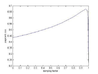
Figure 3: The PageRank mass of IN+SCC as a function of $c$.

Here we see a typical behavior also observed for several pages in the mini-web from [6]: the PageRank first grows with $c$ and then decreases to zero. In our case, the PageRank mass of IN+SCC drops drastically starting from some value $c$ close to one. We can explain this phenomenon by highlighting the role of the dangling nodes.

We start the analysis by subdividing the Web graph sample into three subsets of nodes: IN+SCC, OUT, and the set of dangling nodes DN. We assume that no dangling node originates from OUT. This simplifies the derivation but does not change our conclusions. Then the Web hyper-link matrix $W$ in (1) can be written in the form

$$W=\left[\begin{array}[]{ccc}Q&0&0\\ R&P&S\\ \frac{1}{n}{\bf 1}{\bf 1}^{T}&\frac{1}{n}{\bf 1}{\bf 1}^{T}&\frac{1}{n}{\bf 1}{\bf 1}^{T}\end{array}\right]\;\begin{array}[]{l}\mbox{OUT}\\ \mbox{IN+SCC\;\;,}\\ \mbox{DN}\end{array}$$

where the block $Q$ corresponds to the hyper-links inside the OUT component, the block $R$ corresponds to the hyper-links from IN+SCC to OUT, the block $P$ corresponds to the hyper-links inside the IN+SCC component, and the block $S$ corresponds to the hyper-links from SCC to dangling nodes. In the above, $n$ is the total number of pages in the Web graph sample, and the blocks ${\bf 1}{\bf 1}^{T}$ are the matrices of ones adjusted to appropriate dimensions.

Dividing the PageRank vector in segments corresponding to the blocks OUT, IN+SCC and DN,

$$\pi=[\pi_{\mbox{\tiny OUT}}\,\pi_{\mbox{\tiny IN+SCC}}\,\pi_{\mbox{\tiny DN}}],$$

we can rewrite the well-known formula (see e.g. [18])

$$\pi=\frac{1-c}{n}{\bf 1}^{T}[I-cP]^{-1}$$ (5)

as a system of three linear equations:

$$\pi_{\mbox{\tiny OUT}}[I-cQ]-\pi_{\mbox{\tiny IN+SCC}}cR-\frac{c}{n}\pi_{\mbox{\tiny DN}}{\bf 1}{\bf 1}^{T}=\frac{1-c}{n}{\bf 1}^{T},$$ (6)

$$\pi_{\mbox{\tiny IN+SCC}}[I-cP]-\frac{c}{n}\pi_{\mbox{\tiny DN}}{\bf 1}{\bf 1}^{T}=\frac{1-c}{n}{\bf 1}^{T},$$ (7)

$$-\pi_{\mbox{\tiny IN+SCC}}cS+\pi_{\mbox{\tiny DN}}-\frac{c}{n}\pi_{\mbox{\tiny DN}}{\bf 1}{\bf 1}^{T}=\frac{1-c}{n}{\bf 1}^{T}.$$ (8)

Solving (6–8) for $\pi_{\mbox{\tiny IN+SCC}}$ we obtain

$$\pi_{\mbox{\tiny IN+SCC}}(c)=\frac{(1-c)\alpha}{1-c\beta}{{\bf u}_{\mbox{\tiny IN+SCC}}}\left[I-cP-\frac{c^{2}\alpha}{1-c\beta}S{\bf 1}{{\bf u}_{\mbox{\tiny IN+SCC}}}\right]^{-1},$$ (9)

where

$$\alpha=|IN+SCC|/{n}\quad\mbox{and}\quad\beta=|DN|/{n}$$

are the fractions of nodes in IN+SCC and DN, respectively, and ${{\bf u}_{\mbox{\tiny IN+SCC}}}=|IN+SCC|^{-1}{\bf 1}^{T}$ is a uniform probability row-vector of dimension $|IN+SCC|$. The detailed derivation of (9) can be found in Appendix A.2.

Now, define

$$k(c)=\frac{(1-c)\alpha}{1-c\beta},\quad\mbox{and}\quad U(c)=P+\frac{c\alpha}{1-c\beta}S{\bf 1}{{\bf u}_{\mbox{\tiny IN+SCC}}}.$$ (10)

Then the derivative of $\pi_{\mbox{\tiny IN+SCC}}(c)$ with respect to $c$ is given by

$$\pi^{\prime}_{\mbox{\tiny IN+SCC}}(c)={{\bf u}_{\mbox{\tiny IN+SCC}}}\left\{k^{\prime}(c)I+k(c)[I-cU(c)]^{-1}(cU(c))^{\prime}\right\}[I-cU(c)]^{-1},$$ (11)

where using (10) after simple calculations we get

$$k^{\prime}(c)=-\frac{(1-\beta)\alpha}{(1-c\beta)^{2}},\quad(cU(c))^{\prime}=U(c)+\frac{c\alpha}{(1-c\beta)^{2}}S{\bf 1}{{\bf u}_{\mbox{\tiny IN+SCC}}}.$$

Let us consider the point $c=0$. Using (11), we obtain

$$\pi^{\prime}_{\mbox{\tiny IN+SCC}}(0) = -\alpha(1-\beta){{\bf u}_{\mbox{\tiny IN+SCC}}}+\alpha{{\bf u}_{\mbox{\tiny IN+SCC}}}P.$$ (12)

One can see from the above equation that the PageRank of pages in IN+SCC with many incoming links will increase as $c$ increases from zero, which explains the graphs presented in [6].

Next, let us analyze the total mass of the IN+SCC component. From (12) we obtain

$$||\pi^{\prime}_{\mbox{\tiny IN+SCC}}(0)||=-\alpha(1-\beta){{\bf u}_{\mbox{\tiny IN+SCC}}}+\alpha{{\bf u}_{\mbox{\tiny IN+SCC}}}P{\bf 1}=\alpha(-1+\beta+p_{1}),$$

where $p_{1}={{\bf u}_{\mbox{\tiny IN+SCC}}}P{\bf 1}$ is the probability that a random walk on the hyperlink matrix stays in IN+SCC for one step if the initial distribution is uniform over IN+SCC. If $1-\beta<p_{1}$ then the derivative at 0 is positive. Since dangling nodes typically constitute more than 25% of the graph [19], and $p_{1}$ is usually close to one, the condition $1-\beta<p_{1}$ seems to be comfortably satisfied in Web samples. Thus, the total PageRank of the IN+SCC increases in $c$ when $c$ is small. Note by the way that if $\beta=0$ then $||\pi_{\mbox{\tiny IN+SCC}}(c)||$ is strictly decreasing in $c$. Hence, surprisingly, the presence of dangling nodes qualitatively changes the behavior of the IN+SCC PageRank mass.

Now let us consider the point $c=1$. Again using (11), we obtain

$$\pi^{\prime}_{\mbox{\tiny IN+SCC}}(1)=-\frac{\alpha}{1-\beta}{{\bf u}_{\mbox{\tiny IN+SCC}}}[I-P-\frac{\alpha}{1-\beta}S{\bf 1}{{\bf u}_{\mbox{\tiny IN+SCC}}}]^{-1}.$$ (13)

Note that the matrix in the square braces is close to singular. Denote by $\bar{P}$ the hyper-link matrix of IN+SCC when the outer links are neglected. Then, $\bar{P}$ is an irreducible stochastic matrix. Denote its stationary distribution by $\bar{\pi}_{{\mbox{\tiny IN+SCC}}}$. Then we can apply Lemma A.1 from the singular perturbation theory to (13) by taking

$$A=\bar{P},\quad\varepsilon C=\bar{P}-P-\frac{\alpha}{1-\beta}S{\bf 1}{{\bf u}_{\mbox{\tiny IN+SCC}}},$$

and noting that $\varepsilon C{\bf 1}=R{\bf 1}+(1-\alpha-\beta)(1-\beta)^{-1}S{\bf 1}.$ Combining all terms together and using $\bar{\pi}_{\mbox{\tiny IN+SCC}}{\bf 1}=||\bar{\pi}_{\mbox{\tiny IN+SCC}}||=1$ and ${{\bf u}_{\mbox{\tiny IN+SCC}}}{\bf 1}=||{{\bf u}_{\mbox{\tiny IN+SCC}}}||=1$, from (A.1) we obtain

$$||\pi^{\prime}_{\mbox{\tiny IN+SCC}}(1)|| \approx-\frac{\alpha}{1-\beta}\frac{1}{\bar{\pi}_{\mbox{\tiny IN+SCC}}R{\bf 1}+\frac{1-\beta-\alpha}{1-\beta}\bar{\pi}_{\mbox{\tiny IN+SCC}}S{\bf 1}}.$$

It is expected that the value of $\bar{\pi}_{\mbox{\tiny IN+SCC}}R{\bf 1}+\frac{1-\beta-\alpha}{1-\beta}\bar{\pi}_{\mbox{\tiny IN+SCC}}S{\bf 1}$ is typically small (indeed, in our dataset $INRIA$, the value is 0.022), and hence the mass
$||\pi_{\mbox{\tiny IN+SCC}}(c)||$ decreases very fast as $c$ approaches one.

Having described the behavior of the PageRank mass $||\pi_{\mbox{\tiny IN+SCC}}(c)||$ at the boundary points $c=0$ and $c=1$, now we would like to show that there is at most one extremum on $(0,1)$. It is sufficient to prove that if $||\pi_{\mbox{\tiny IN+SCC}}^{\prime}(c_{0})||\leq 0$ for some $c_{0}\in(0,1)$ then $||\pi_{\mbox{\tiny IN+SCC}}^{\prime}(c)||\leq 0$ for all $c>c_{0}$. To this end, we apply the Sherman-Morrison formula to (9), which yields

$$\pi_{\mbox{\tiny IN+SCC}}(c)=\tilde{\pi}_{\mbox{\tiny IN+SCC}}(c)+\frac{\frac{c^{2}\alpha}{1-c\beta}{{\bf u}_{\mbox{\tiny IN+SCC}}}[I-cP]^{-1}S{\bf 1}}{1+\frac{c^{2}\alpha}{1-c\beta}{{\bf u}_{\mbox{\tiny IN+SCC}}}[I-cP]^{-1}S{\bf 1}}\,\tilde{\pi}_{\mbox{\tiny IN+SCC}}(c),$$ (14)

where

$$\tilde{\pi}_{{\mbox{\tiny IN+SCC}}}(c)=\frac{(1-c)\alpha}{1-c\beta}{{\bf u}_{\mbox{\tiny IN+SCC}}}[I-cP]^{-1}.$$ (15)

represents the main term in the right-hand side of (14). (The second summand in (14) is about 10% of the total sum for the $INRIA$ dataset for $c=0.85$.) Now the behavior of $\pi_{\mbox{\tiny IN+SCC}}(c)$ in Figure 3 can be explained by means of the next proposition (see Appendix A.2 for the proof).

Proposition 2

The term $||\tilde{\pi}_{\mbox{\tiny IN+SCC}}(c)||$ given by (15) has exactly one local maximum at some $c_{0}\in[0,1]$. Moreover, $||\tilde{\pi}^{\prime\prime}_{\mbox{\tiny IN+SCC}}(c)||<0$ for $c\in(c_{0},1]$.

We conclude that $||\tilde{\pi}_{\mbox{\tiny IN+SCC}}(c)||$ is decreasing and concave for $c\in[c_{0},1]$, where $||\tilde{\pi}^{\prime}_{\mbox{\tiny IN+SCC}}(c_{0})||=0$. This is exactly the behavior we observe in the experiments. The analysis and experiments suggest that $c_{0}$ is definitely larger than 0.85 and actually is quite close to one. Thus, one may want to choose large $c$ in order to maximize the PageRank mass of IN+SCC. However, in the next section we will indicate important drawbacks of this choice.

5 PageRank mass of ESCC

Let us now consider the PageRank mass of the Extended SCC component (ESCC) described in Section 3, as a function of $c\in[0,1]$. Subdividing the PageRank vector in the blocks $\pi=[\pi_{{\mbox{\tiny PureOUT}}}\;\pi_{\mbox{\tiny ESCC}}]$, from (5) we obtain

$$||\pi_{\mbox{\tiny ESCC}}(c)|| =(1-c)\gamma{{\bf u}_{\mbox{\tiny ESCC}}}[I-cT]^{-1}{\bf 1},$$ (16)

where $T$ represents the transition probabilitites inside the ESCC block, $\gamma=|ESCC|/n$, and ${{\bf u}_{\mbox{\tiny ESCC}}}$ is a uniform probability row-vector over ESCC. Clearly, we have $||\pi_{\mbox{\tiny ESCC}}(0)||=\gamma$ and $||\pi_{\mbox{\tiny ESCC}}(1)||=0$. Furthermore, by taking derivatives we easily show that $||\pi_{\mbox{\tiny ESCC}}(c)||$ is a concave decreasing function. In the next proposition (proved in the Appendix), we derive a series of bounds for $||\pi_{\mbox{\tiny ESCC}}(c)||$.

Proposition 3

Let $\lambda_{1}$ be the Perron-Frobenius eigenvalue of $T$, and let $p_{1}={{\bf u}_{\mbox{\tiny ESCC}}}T{\bf 1}$ be the probability that the random walk started from a randomly chosen state in ESCC, stays in ESCC for one step.

• If $p_{1}<\lambda_{1}$ then

  $$||\pi_{\mbox{\tiny ESCC}}(c)||<\frac{\gamma(1-c)}{1-c\lambda_{1}},\quad c\in(0,1).$$ (17)

• If $1/(1-p_{1})<{{\bf u}_{\mbox{\tiny ESCC}}}[I-T]^{-1}{\bf 1}$ then

  $$||\pi_{\mbox{\tiny ESCC}}(c)||>\frac{\gamma(1-c)}{1-cp_{1}},\quad c\in(0,1).$$ (18)

The condition $p_{1}<\lambda_{1}$ has a clear intuitive interpretation. Let $\hat{\pi}_{\mbox{\tiny ESCC}}$ be the probability-normed left Perron-Frobenius eigenvector of $T$. Then $\hat{\pi}_{\mbox{\tiny ESCC}}$, also known as a quasi-stationary distribution of $T$, is the limiting probability distribution of the Markov chain given that the random walk never leaves the block $T$ (see e.g.  [20]). Since $\hat{\pi}_{\mbox{\tiny ESCC}}T=\lambda_{1}$, the condition $p_{1}<\lambda_{1}$ means that the chance to stay in ESCC for one step in the quasi-stationary regime is higher than starting from the uniform distribution ${{\bf u}_{\mbox{\tiny ESCC}}}$. Although $p_{1}<\lambda_{1}$ does not hold in general, one may expect that it should hold for transition matrices describing large entangled graphs since quasi-stationary distribution should favor states, from which the chance to leave ESCC is lower.

Both conditions of Proposition 3 are satisfied in our experiments. With the help of the derived bounds we conclude that $||\pi_{\mbox{\tiny ESCC}}(c)||$ decreases very slowly for small and moderate values of $c$, and it decreases extremely fast when $c$ becomes close to 1. This typical behavior is clearly seen in Figure 4, where $||\pi_{\mbox{\tiny ESCC}}(c)||$ is plotted with a solid line.

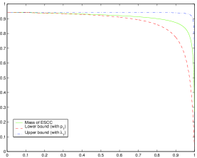
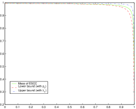
Figure 4: PageRank mass of ESCC and bounds, INRIA (left) and FrMathInfo (right)

The bounds are plotted in Figure 4 with dashed lines. For the INRIA dataset we have $p_{1}=0.97557$, $\lambda_{1}=0.99954$, and for the FrMathInfo dataset we have $p_{1}=0.99659$, $\lambda_{1}=0.99937$.

From the above we conclude that the PageRank mass of ESCC is smaller than $\gamma$ for any value $c>0$. On contrary, the PageRank mass of Pure OUT increases in $c$ beyond its “fair share” $\delta=|PureOUT|/n$. With $c=0.85$, the PageRank mass of the Pure OUT component in the INRIA dataset is equal to $1.95\delta$. In the FrMathInfo dataset, the unfairness is even more pronounced: the PageRank mass of the Pure OUT component is equal to $3.44\delta$. This gives users an incentive to create dead-ends: groups of pages that link only to each other. Clearly, this can be mitigated by choosing a smaller damping factor. Below we propose one way to determine an “optimal” value of $c$.

Let ${\bf v}$ be some probability vector over ESCC. We would like to choose $c=c^{*}$ that satisfies the condition

$$||\pi_{\mbox{\tiny ESCC}}(c)||=||{\bf v}T||,$$ (19)

that is, starting from ${\bf v}$, the probability mass preserved in ESCC after one step should be equal to the PageRank of ESCC. One can think for instance of the following three reasonable choices of ${\bf v}$: 1) $\hat{\pi}_{T}$, the quasi-stationary distribution of $T$, 2) the uniform vector ${{\bf u}_{\mbox{\tiny ESCC}}}$, and 3) the normalized PageRank vector $\pi_{\mbox{\tiny ESCC}}(c)/||\pi_{\mbox{\tiny ESCC}}(c)||$. The first choice reflects the proximity of $T$ to a stochastic matrix. The second choice is inspired by definition of PageRank (restart from uniform distribution), and the third choice combines both these features.

If conditions of Proposition 3 are satisfied, then (17) and (18) hold, and thus the value of $c^{*}$ satisfying (19) must be in the interval $(c_{1},c_{2})$, where

$$(1-c_{1})/(1-p_{1}c_{1})=||{\bf v}T||,\quad(1-c_{2})/(1-\lambda_{1}c_{2})=||{\bf v}T||.$$

Numerical results for all three choices of ${\bf v}$ are presented in Table 1.

$v$ $c$ INRIA FrMathInfo $\hat{\pi}_{\mbox{\tiny ESCC}}$ $c_{1}$ 0.0184 0.1956 $c_{2}$ 0.5001 0.5002 $c^{*}$ .02 .16 ${{\bf u}_{\mbox{\tiny ESCC}}}$ $c_{1}$ 0.5062 0.5009 $c_{2}$ 0.9820 0.8051 $c^{*}$ .604 .535 $\pi_{\mbox{\tiny ESCC}}/||\pi_{\mbox{\tiny ESCC}}||$ $1/(1+\lambda_{1})$ 0.5001 0.5002 $1/(1+p_{1})$ 0.5062 0.5009

Table 1: Values of $c^{*}$ with bounds.

If ${\bf v}=\hat{\pi}_{\mbox{\tiny ESCC}}$ then we have $||{\bf v}T||=\lambda_{1}$, which implies $c_{1}=(1-\lambda_{1})/(1-\lambda_{1}p_{1})$ and $c_{2}=1/(\lambda_{1}+1)$. In this case, the upper bound $c_{2}$ is only slightly larger than $1/2$ and $c^{*}$ is close to zero in our data sets (see Tabel 1). Such small $c$ however leads to ranking that takes into account only local information about the Web graph (see e.g. [21]). The choice ${\bf v}=\hat{\pi}_{\mbox{\tiny ESCC}}$ does not seem to represent the dynamics of the system; probably because the “easily bored surfer” random walk that is used in PageRank computations never follows a quasi-stationary distribution since it often restarts itself from the uniform probability vector.

For the uniform vector ${\bf v}={{\bf u}_{\mbox{\tiny ESCC}}}$, we have $||{\bf v}T||=p_{1}$, which gives $c_{1},c_{2},c^{*}$ presented in Table 1. We have obtained a higher upper bound but the values of $c^{*}$ are still much smaller than $0.85$.

Finally, for the normalized PageRank vector ${\bf v}=\pi_{\mbox{\tiny ESCC}}/||\pi_{\mbox{\tiny ESCC}}||$, using (16), we rewrite (19) as

$$||\pi_{\mbox{\tiny ESCC}}(c)|| =\frac{\gamma}{||\pi_{\mbox{\tiny ESCC}}(c)||}\pi_{\mbox{\tiny ESCC}}(c)T{\bf 1}=\frac{\gamma^{2}(1-c)}{||\pi_{\mbox{\tiny ESCC}}(c)||}{{{\bf u}_{\mbox{\tiny IN+SCC}}}}[I-cT]^{-1}T{\bf 1},$$

Multiplying by $||\pi_{\mbox{\tiny ESCC}}(c)||$, after some algebra we obtain

$$||\pi_{\mbox{\tiny ESCC}}(c)||^{2} =\frac{\gamma}{c}\,||\pi_{\mbox{\tiny ESCC}}(c)||-\frac{(1-c)\gamma^{2}}{c}.$$

Solving the quadratic equation for $||\pi_{\mbox{\tiny ESCC}}(c)||$, we get

$$||\pi_{\mbox{\tiny ESCC}}(c)||=r(c)=\left\{\begin{array}[]{ll}\gamma&\mbox{if }c\leq 1/2,\\ \frac{\gamma(1-c)}{c}&\mbox{if }c>1/2.\end{array}\right.$$

Hence, the value $c^{*}$ solving (19) corresponds to the point where the graphs of $||\pi_{\mbox{\tiny ESCC}}(c)||$ and $r(c)$ cross each other. There is only one such point on (0,1), and since $||\pi_{\mbox{\tiny ESCC}}(c)||$ decreases very slowly unless $c$ is close to one, whereas $r(c)$ decreases relatively fast for $c>1/2$, we expect that $c^{*}$ is only slightly larger than $1/2$. Under conditions of Proposition 3, $r(c)$ first crosses the line $\gamma(1-c)/(1-\lambda_{1}c)$, then $||\pi_{T}(c)||_{1}$, and then $\gamma(1-c)/(1-p_{1}c)$. Thus, we yield $(1+\lambda_{1})^{-1}<c^{*}<(1+p_{1})^{-1}$. Since both $\lambda_{1}$ and $p_{1}$ are large, this suggests that $c$ should be chosen around 1/2. This is also reflected in Tabel 1.

Last but not least, to support our theoretical argument about the undeserved high ranking of pages from Pure OUT, we carry out the following experiment. In the $INRIA$ dataset we have chosen an absorbing component in Pure OUT consisting just of two nodes. We have added an artificial link from one of these nodes to a node in the Giant SCC and recomputed the PageRank. In Table 2 in the column “PR rank w/o link” we give a ranking of a page according to the PageRank value computed before the addition of the artificial link and in the column “PR rank with link” we give a ranking of a page according to the PageRank value computed after the addition of the artificial link. We have also analyzed the log file of the site INRIA Sophia Antipolis (www-sop.inria.fr) and ranked the pages according to the number of clicks for the period of one year up to May 2007. We note that since we have the access only to the log file of the INRIA Sophia Antipolis site, we use the PageRank ranking also only for the pages from the INRIA Sophia Antipolis site. For instance, for $c=0.85$, the ranking of Page A without an artificial link is 731 (this means that 731 pages are ranked better than Page A among the pages of INRIA Sophia Antipolis). However, its ranking according to the number of clicks is much lower, 2588. This confirms our conjecture that the nodes in Pure OUT obtain unjustifiably high ranking. Next we note that the addition of an artificial link significantly diminishes the ranking. In fact, it brings it close to the ranking provided by the number of clicks. Finally, we draw the attention of the reader to the fact that choosing $c=1/2$ also significantly reduces the gap between the ranking by PageRank and the ranking by the number of clicks.

$c$ PR rank w/o link PR rank with link rank by no. of clicks Node A 0.5 1648 2307 2588 0.85 731 2101 2588 0.95 226 2116 2588 Node B 0.5 1648 4009 3649 0.85 731 3279 3649 0.95 226 3563 3649

Table 2: Comparison between PR and click based rankings.

To summarize, our results indicate that with $c=0.85$, the Pure OUT component receives an unfairly large share of the PageRank mass. Remarkably, in order to satisfy any of the three intuitive criteria of fairness presented above, the value of $c$ should be drastically reduced. The experiment with the log files confirms the same. Of course, a drastic reduction of $c$ also considerably accelerates the computation of PageRank by numerical methods [22, 5, 23].

Appendix

A.1 Results from Singular Perturbation Theory

Lemma A.1

Let $A(\varepsilon)=A-\varepsilon C$ be a perturbation of irreducible stochastic matrix $A$ such that $A(\varepsilon)$ is substochastic. Then, for sufficiently small $\varepsilon$ the following Laurent series expansion holds

$$[I-A(\varepsilon)]^{-1}=\frac{1}{\varepsilon}X_{-1}+X_{0}+\varepsilon X_{1}+...\ ,$$

with

$$X_{-1}=\frac{1}{\mu C{\bf 1}}{\bf 1}\mu,$$

where $\mu$ is the stationary distribution of $A$. It follows that

$$[I-A(\varepsilon)]^{-1}=\frac{1}{\mu\varepsilon C{\bf 1}}{\bf 1}\mu+\mbox{O}(1)\quad\mbox{as }\varepsilon\to 0.$$ (A.1)

Lemma A.2

Let $A(\varepsilon)=A+\varepsilon C$ be a transition matrix of perturbed Markov chain.

The perturbed Markov chain is assumed to be ergodic for sufficiently small $\varepsilon$ different from zero. Let the unperturbed Markov chain $(\varepsilon=0)$ have $m$ ergodic classes. Namely, the transition matrix $A$ can be written in the form

$$A=\left[\begin{array}[]{cccc}A_{1}&&0&0\\ &\ddots&&\\ 0&&A_{m}&0\\ L_{1}&\cdots&L_{m}&E\end{array}\right]\in\mathbb{R}^{n\times n}.$$

Then, the stationary distribution of the perturbed Markov chain has a limit

$$\lim_{\varepsilon\to 0}\pi(\varepsilon)=[\nu_{1}\mu_{1}\ \cdots\ \nu_{m}\mu_{m}\ 0],$$

where zeros correspond to the set of transient states in the unperturbed Markov chain, $\mu_{i}$ is a stationary distribution of the unperturbed Markov chain corresponding to the $i$-th ergodic set, and $\nu_{i}$ is the $i$-th element of the aggregated stationary distribution vector that can be found by solution

$$\nu D=\nu,\quad\nu{\bf 1}=1,$$

where $D=MCB$ is the generator of the aggregated Markov chain and

$$M=\left[\begin{array}[]{cccc}\mu_{1}&&0&0\\ &\ddots&&\\ 0&&\mu_{m}&0\end{array}\right]\in\mathbb{R}^{m\times n},\quad B=\left[\begin{array}[]{cccc}{\bf 1}&&0\\ &\ddots&\\ 0&&{\bf 1}\\ \phi_{1}&\cdots&\phi_{m}\end{array}\right]\in\mathbb{R}^{n\times m}.$$

with $\phi_{i}=[I-E]^{-1}L_{i}{\bf 1}$.

The proof of this lemma can be found in [11, 12, 14].

A.2 Proofs

Derivation of (9). First, we observe that if $\pi_{\mbox{\tiny IN+SCC}}$ and $\pi_{\mbox{\tiny DN}}{\bf 1}$ are known then it is straightforward to calculate $\pi_{\mbox{\tiny OUT}}$. Namely, we have

$$\pi_{\mbox{\tiny OUT}}=\pi_{\mbox{\tiny IN+SCC}}cR[I-cQ]^{-1}+\left(\frac{1-c}{n}+\pi_{\mbox{\tiny DN}}{\bf 1}\frac{c}{n}\right){\bf 1}^{T}[I-cQ]^{-1}.$$

Therefore, let us solve the equations (7) and (8). Towards this goal, we sum the elements of the vector equation (8), which corresponds to the postmultiplication of equation (8) by vector ${\bf 1}$.

$$-\pi_{\mbox{\tiny IN+SCC}}cS{\bf 1}+\pi_{\mbox{\tiny DN}}{\bf 1}-\frac{c}{n}\pi_{\mbox{\tiny DN}}{\bf 1}{\bf 1}^{T}{\bf 1}=\frac{1-c}{n}{\bf 1}^{T}{\bf 1}$$

Now, denote by $n_{OUT}$, $n_{SCC}$ and $n_{DN}$ the number of pages in OUT component, SCC component and the number of dangling nodes. Since ${\bf 1}^{T}{\bf 1}=n_{DN}$, we have

$$\pi_{\mbox{\tiny DN}}{\bf 1}=\frac{n}{n-cn_{DN}}(\pi_{\mbox{\tiny IN+SCC}}cS{\bf 1}+\frac{1-c}{n}n_{DN}).$$

Substituting the above expression for $\pi_{\mbox{\tiny DN}}{\bf 1}$ into (7), we get

$$\pi_{\mbox{\tiny IN+SCC}}\left[I-cP-\frac{c^{2}}{n-cn_{DN}}S{\bf 1}{\bf 1}^{T}\right]=\frac{c}{n-cn_{DN}}\frac{1-c}{n}n_{DN}{\bf 1}^{T}+\frac{1-c}{n}{\bf 1}^{T},$$

which directly implies (9).

Proof of Proposition 1 First, we note that if we make a change of variables $\varepsilon=1-c$ the Google matrix becomes a transition matrix of a singularly perturbed Markov chain as in Lemma A.2 with $C=\frac{1}{n}{\bf 1}{\bf 1}^{T}-P$. Let us calculate the aggregated generator matrix $D$:

$$D=MCQ=\frac{1}{n}{\bf 1}{\bf 1}^{T}Q-MPQ.$$

Using $MP=M$, $MQ=I$, and $M{\bf 1}={\bf 1}$ where vectors ${\bf 1}$ are of appropriate dimensions, we obtain

$$D =\frac{1}{n}{\bf 1}{\bf 1}^{T}Q-I=\frac{1}{n}{\bf 1}[n_{1}+{\bf 1}[I-{T}]^{-1}{R}_{1}{\bf 1},\cdots,n_{m}+{\bf 1}[I-\tilde{T}]^{-1}{R}_{m}{\bf 1}]-I,$$

where $n_{i}$ be the number of nodes in the block $Q_{i}$, $i=1,\ldots,m$. Since the aggregated transition matrix $D+I$ has identical rows, its stationary distribution $\nu$ is just equal to these rows. Thus, invoking Lemma A.2 we obtain (4).

Proof of Proposition 2 Multiplying both sides of (15) by ${\bf 1}$ and taking the derivatives, after some tedious algebra we obtain

$$||\tilde{\pi}^{\prime}_{\mbox{\tiny IN+SCC}}(c)||= -a(c)+\frac{\beta}{1-c\beta}\,||\tilde{\pi}_{scc}(c)||,$$ (A.2)

where the real-valued function $a(c)$ is given by

$$a(c)=\frac{\alpha}{1-c\beta}{{\bf u}_{\mbox{\tiny IN+SCC}}}[I-cP]^{-1}[I-P][I-cP]^{-1}{\bf 1}.$$

Differentiating (A.2) and substituting $\frac{\beta}{1-c\beta}||\tilde{\pi}_{SCC}(c)||$ from (A.2) in the resulting expression, we get

$$||\tilde{\pi}^{\prime\prime}_{\mbox{\tiny IN+SCC}}(c)|| =\left\{-a^{\prime}(c)+\frac{\beta}{1-c\beta}a(c)\right\}+\frac{2\beta}{1-c\beta}\,||\tilde{\pi}^{\prime}_{SCC}(c)||.$$

Note that the term in the curly braces is negative by definition of $a(c)$. Hence, if $||\tilde{\pi}^{\prime}_{\mbox{\tiny IN+SCC}}(c)||\leq 0$ for some $c\in[0,1]$ then $||\tilde{\pi}^{\prime\prime}_{\mbox{\tiny IN+SCC}}(c)||<0$ for this value of $c$.

Proof of Proposition 3 (i) The function $f(c)=\gamma(1-c)/(1-\lambda_{1}c)$ is decreasing and concave, and so is $||\pi_{\mbox{\tiny ESCC}}(c)||$. Also, $||\pi_{\mbox{\tiny ESCC}}(0)||=f(0)=\gamma$, and $||\pi_{\mbox{\tiny ESCC}}(1)||=f(1)=0$. Thus, for $c\in(0,1)$, the plot of $||\pi_{\mbox{\tiny ESCC}}(c)||$ is either entirely above or entirely below $f(c)$. In particular, if the first derivatives satisfy $||\pi^{\prime}_{\mbox{\tiny ESCC}}(0)||<f^{\prime}(0)$, then $||\pi_{\mbox{\tiny ESCC}}(c)||<f(c)$ for any $c\in(0,1)$. Since $f^{\prime}(0)=\gamma(\lambda_{1}-1)$ and $||\pi^{\prime}_{\mbox{\tiny ESCC}}(0)||=\gamma(p_{1}-1)$, we see that $p_{1}<\lambda_{1}$ implies (17).

The proof of (ii) is similar. We consider a concave decreasing function $g(c)=\gamma(1-c)/(1-p_{1}c)$ and note that $g(0)=\gamma$, $g(1)=0$. Now, if the condition in (ii) holds then $g^{\prime}(1)>||\pi^{\prime}_{\mbox{\tiny ESCC}}(1)||$, which implies (18).

References

- [1] Page, L., Brin, S., Motwani, R., Winograd, T.: The PageRank citation ranking: Bringing order to the web. Technical report, Stanford University (1998)
- [2] Kleinberg, J.M.: Authoritative sources in a hyperlinked environment. Journal of the ACM 46(5) (1999) 604–632
- [3] Lempel, R., Moran, S.: The stochastic approach for link-structure analysis (SALSA) and the TKC effect. Comput. Networks 33(1–6) (2000) 387–401
- [4] Langville, A.N., Meyer, C.D.: Deeper inside PageRank. Internet Math. 1 (2003) 335–380
- [5] Langville, A.N., Meyer, C.D.: Google’s PageRank and beyond: the science of search engine rankings. Princeton University Press, Princeton, NJ (2006)
- [6] Boldi, P., Santini, M., Vigna, S.: PageRank as a function of the damping factor. In: Proc. of the Fourteenth International World Wide Web Conference, Chiba, Japan, ACM Press (2005)
- [7] Avrachenkov, K., Litvak, N.: The effect of new links on Google PageRank. Stoch. Models 22(2) (2006) 319–331
- [8] Bianchini, M., Gori, M., Scarselli, F.: Inside PageRank. ACM Trans. Inter. Tech. 5(1) (2005) 92–128
- [9] Broder, A., Kumar, R., Maghoul, F., Raghavan, P., Rajagopalan, S., Statac, R., Tomkins, A., J.Wiener: Graph structure in the Web. Computer Networks 33 (2000) 309–320
- [10] Kumar, R., Raghavan, P., Rajagopalan, S., Sivakumar, D., Tomkins, A., Upfal, E.: The Web as a graph. In: Proc. 19th ACM SIGACT-SIGMOD-AIGART Symp. Principles of Database Systems, PODS, ACM Press (15–17 2000) 1–10
- [11] Avrachenkov, K.: Analytic Perturbation Theory and its Applications. PhD thesis, University of South Australia (1999)
- [12] Korolyuk, V.S., Turbin, A.F.: Mathematical foundations of the state lumping of large systems. Volume 264 of Mathematics and its Applications. Kluwer Academic Publishers Group, Dordrecht (1993)
- [13] Pervozvanskii, A.A., Gaitsgori, V.G.: Theory of suboptimal decisions. Volume 12 of Mathematics and its Applications (Soviet Series). Kluwer Academic Publishers Group, Dordrecht (1988)
- [14] Yin, G.G., Zhang, Q.: Discrete-time Markov chains. Volume 55 of Applications of Mathematics (New York). Springer-Verlag, New York (2005)
- [15] Chen, P., Xie, H., Maslov, S., Redner, S.: Finding scientific gems with google. Arxiv preprint physics/0604130 (2006)
- [16] Dill, S., Kumar, R., Mccurley, K.S., Rajagopalan, S., Sivakumar, D., Tomkins, A.: Self-similarity in the web. ACM Trans. Inter. Tech. 2(3) (2002) 205–223
- [17] Haveliwala, T.: Topic-sensitive PageRank: A context-sensitive ranking algorithm for Web search. IEEE Transactions on Knowledge and Data Engineering 15(4) (2003) 784–796
- [18] Moler, C., Moler, K.: Numerical Computing with MATLAB. SIAM (2003)
- [19] Eiron, N., McCurley, K., Tomlin, J.: Ranking the Web frontier. In: WWW ’04: Proceedings of the 13th international conference on World Wide Web, New York, NY, USA, ACM Press (2004) 309–318
- [20] Seneta, E.: Non-negative matrices and Markov chains. Springer Series in Statistics. Springer, New York (2006) Revised reprint of the second (1981) edition [Springer-Verlag, New York; MR0719544].
- [21] Fortunato, S., Flammini, A.: Random walks on directed networks: the case of PageRank. Technical Report 0604203, arXiv/physics (2006)
- [22] Avrachenkov, K., Litvak, N., Nemirovsky, D., Osipova, N.: Monte Carlo methods in PageRank computation: When one iteration is sufficient. SIAM J. Numer. Anal. (2007)
- [23] Berkhin, P.: A survey on PageRank computing. Internet Math. 2 (2005) 73–120