Converting H$\alpha$ luminosities into star formation rates

Abstract

Star-formation rates (SFRs) of galaxies are commonly calculated by converting the measured H$\alpha$ luminosities ($L_{\mathrm{H\alpha}}$) into current SFRs. This conversion is based on a constant initial mass function (IMF) independent of the total SFR. As recently recognised the maximum stellar mass in a star cluster is limited by the embedded total cluster mass and, in addition, the maximum embedded star cluster mass is constrained by the current SFR. The combination of these two relations leads to an integrated galaxial initial stellar mass function (IGIMF, the IMF for the whole galaxy) which is steeper in the high mass regime than the constant canonical IMF, and is dependent on the SFR of the galaxy. Consequently, the $L_{\mathrm{H\alpha}}$-SFR relation becomes non-linear and flattens for low SFRs. Especially for dwarf galaxies the SFRs can be underestimated by up to three orders of magnitude. We revise the existing linear $L_{\mathrm{H}\alpha}$-SFR relations using our IGIMF notion. These are likely to lead to a revision of the cosmological star formation histories. We also demonstrate that in the case of the Sculptor dwarf irregular galaxies the IGIMF-formalism implies a linear dependence of the total SFR on the total galaxy gas mass. A constant gas depletion time scale of a few Gyrs results independently of the galaxy gas mass with a reduced scatter compared to the conventional results. Our findings are qualitatively independent of the explicit choice of the IGIMF details and challenges current star formation theory in dwarf galaxies.

1 Introduction

Low-mass dwarf galaxies are very important objects to test the theoretical understanding of star formation, galactic evolution and cosmology. One key issue in this process is the accurate determination of current SFRs. Because massive stars have short life times the number of currently existing massive stars determines the actual massive star formation rate. The number of massive stars is commonly obtained from the integrated H$\alpha$ luminosity of the target galaxy, after correcting the observations for extinction and N ii emission. If the fraction of massive star formation of the total star formation is known then the meassured integrated H$\alpha$ luminosity of a galaxy can be converted into its current SFR.

The standard method is to apply one initial mass function (IMF) to the entire population of newly formed stars in the whole galaxy. This standard method provides a linear relation between the integrated H$\alpha$ luminosity and the current SFR (Kennicutt, 1983; Kennicutt et al., 1994; Kennicutt, 1998). Originally used for normal disk galaxies such linear relations have also been applied to dwarf irregular galaxies (Skillman et al., 2003).

But even if star formation in each young star cluster follows the same canonical IMF (Kroupa, 2001, 2002; Pflamm-Altenburg & Kroupa, 2006), the total stellar population of newly formed stars of all young star clusters together follows a distribution function which is steeper than the canonical IMF in the high mass regime (Kroupa & Weidner, 2003; Weidner & Kroupa, 2005). This distribution function is called the integrated galaxial initial stellar mass function (IGIMF) and deviates increasingly from the underlying canonical IMF with decreasing galactic-wide star formation and total galaxy mass (Weidner & Kroupa, 2005).

This effect has undoubtedly consequences for the cosmological evolution of the number of supernovae per low-mass star and the chemical enrichment of galaxies of different mass. As a first step the formulation of the IGIMF has been successfully used to naturally explain the mass-metallicity relation of galaxies (Köppen, Weidner & Kroupa, 2007).

Observational evidence supporting this IGIMF concept has been published by Selman & Melnick (2005) who find a steeper IMF-slope of the high-mass regime in the field population of 30 Doradus than in the cluster NGC 2070 as predicted by Kroupa & Weidner (2003). Note that the Scalo (1986) Milky-Way-disc IMF index $\alpha\approx 2.7$ (Kroupa, Tout & Gilmore, 1993) is larger than the canonical IMF index $\alpha\approx 2.35$. This difference is a natural consequence of the IGIMF notion (Kroupa & Weidner, 2003). Using the Scalo index Diehl et al. (2006) find a consistency of the supernova rate derived from the Galactic ²⁶Al gamma-ray flux and deduced from a survey from local O and B stars, extrapolated to the whole Galaxy (McKee & Williams, 1997). Noteworthy is the finding by Lee et al. (2004) that LSB galaxies have much steeper than Salpeter massive-star IMFs than Milky-Way-type galaxies, as expected from the IGIMF formalism. Hoversten & Glazebrook (2007) find evidence for a non-universal stellar IMF from the integrated properties of SDSS galaxies. Bright galaxies have a high-massive star slope of $\approx 2.4$, whereas fainter galaxies prefer steeper IMFs. The observed effect is very much in-line with the theoretical predictions of Weidner & Kroupa (2005).

For a given global SFR the total number of massive stars based on an IGIMF is less than in the standard procedure. Thus, the expected IGIMF-H$\alpha$ luminosity is less than the H$\alpha$ luminosity calculated in the standard way, implying that SFRs of galaxies determined by the standard method are systematically underestimated.

After a summary of the IGIMF basics we develop for different IGIMF-models a relation between the SFR and the produced H$\alpha$ luminosity and provide easy-to-use fitting functions (Sec. 2). In Sec. 3 we apply our $L_{\mathrm{H}\alpha}$-SFR relation to the dwarf irregular galaxies in the Sculptor cluster and discuss the changes of some of their parameters. Finally, we explore the detection limits for star formation (Sec. 4).

2 SFR-L_Hα-relation

For a given SFR we assume that star formation takes place in star clusters distributed according to a mass function which is called the embedded cluster mass function (ECMF) of stellar masses (i.e. the function of the stellar-mass content in clusters before they expel their residual gas), $\xi_{\mathrm{ecl}}(M_{\mathrm{cl}})$. These star clusters are formed within a time-span, $\delta t$, which is called the ”star-formation epoch” of the galaxy (Weidner & Kroupa, 2005).

The total mass of all formed stars, $M_{\mathrm{SFR}}$, in all star clusters within the epoch $\delta t$ is then given by

$$M_{\mathrm{SFR}}=\mathrm{SFR}\;\;\delta t=\int_{M_{\mathrm{ecl,min}}}^{M_{\mathrm{ecl,max}}}M_{\mathrm{ecl}}\;\xi_{\mathrm{ecl}}(M_{\mathrm{ecl}})\;\mathrm{d}M_{\mathrm{ecl}}\;\;\;,$$ (1)

where $M_{\mathrm{ecl,min}}$ and $M_{\mathrm{ecl,max}}$ are, respectively, the least-massive and most-massive embedded cluster able to form. The total ensemble of all newly formed stars has a mass spectrum described by the IGIMF, $\xi_{\mathrm{IGIMF}}(m)$, constructed below. A star with the mass $m$ produces a total number, $N_{\mathrm{ion},\delta t}(m)$, of ionising photons during the epoch $\delta t$. The total number of ionising photons emitted by all young stars within $\delta t$ is given by

$$N_{\mathrm{ion},\delta t}=\int_{m_{\mathrm{low}}}^{m_{\mathrm{max}}}\xi_{\mathrm{IGIMF}}(m)\;N_{\mathrm{ion},\delta t}(m)\;\mathrm{d}m\;\;\;,$$ (2)

where $m_{\mathrm{low}}$ and $m_{\mathrm{max}}$ are, respectively, the minimum and maximum stellar mass. The calculation of $N_{\mathrm{ion},\delta t}$ will be described in Sec. 2.2.

Assuming that a fraction, $\mu$, of all ionising photons leads to H$\alpha$ emission in the surrounding gas then the resulting H$\alpha$ luminosity is

$$L_{\mathrm{H\alpha}}=\mu\;3.0207\cdot 10^{-12}\;\mathrm{erg}\;N_{\mathrm{ion}}/\delta t\;\;\;,$$ (3)

where the energy of one H$\alpha$-photon is $3.0207\cdot 10^{-12}$ erg. Throughout this paper we assume $\mu=1$. It can be argued that the time-span $\delta t$ can be removed in this formulation by considering rates directly. But the total mass, $M_{\mathrm{SFR}}$, defined by Eq. 1 and depending explicitly on $\delta t$, is an upper limit of the ECMF, as no cluster can be formed more massive than the available material.

2.1 IGIMF

Larsen (2000, 2002b, 2002a) and Larsen & Richtler (2000) found that the V-band luminosity of the brightest young cluster correlates with the global SFR. Based on the conclusion by Larsen (2002b) that the so-called super-clusters are just the young and massive upper end of a cluster mass function, Weidner et al. (2004) derived a relation between the maximum embedded cluster mass, $M_{\mathrm{ecl,max}}$, in a galaxy and the current global SFR

$$\log_{10}\left(M_{\mathrm{ecl,max}}\right)=\log_{10}\left(k_{\mathrm{ML}}\right)+0.75\cdot\log_{10}\left(\mathrm{SFR}\right)+6.77\;\;\;,$$ (4)

where $k_{\mathrm{ML}}$ is the mass-to-light ratio, typically 0.0144 for young ($<$ 6 Myr) stellar populations. They showed that this relation can be reproduced theoretically if the ECMF is a power-law with a slope of 2.35 and the entire star cluster population ranging from $M_{\mathrm{ecl,min}}\approx$ 5 M_⊙ to $M_{\mathrm{ecl,max}}$ is born within a time-span of $\delta t\approx$ 10 Myr, independently of the SFR. The concept of a relation between the SFR of a galaxy and the mass of the most massive star cluster has been developed further to derive the star formation history of galaxies (Maschberger & Kroupa, 2007).

Each cluster with the mass $M_{\mathrm{ecl}}$ then forms $N$ stars between the mass limits $m_{\mathrm{low}}$ and $m_{\mathrm{max}}$ according to the canonical IMF,

$$N=\int_{m_{\mathrm{low}}}^{m_{\mathrm{max}}}\xi_{M_{\mathrm{ecl}}}(m)\mathrm{d}m\;\;\;.$$ (5)

This canonical IMF, $\xi_{M_{\mathrm{ecl}}}(m)$, is a two-part-power law and is here calculated using the algorithm by Pflamm-Altenburg & Kroupa (2006). The normalisation constant of the IMF in an individual cluster, $\xi_{M_{\mathrm{ecl}}}(m)$, with the mass $M_{\mathrm{ecl}}$ and the maximum stellar mass, $m_{\mathrm{max}}$, in this star cluster are determined by the two equations (Weidner & Kroupa, 2004)

$$M_{\mathrm{ecl}}=\int_{m_{\mathrm{low}}}^{m_{\mathrm{max}}}m\;\xi_{M_{\mathrm{ecl}}}(m)\mathrm{d}m\;\;\;,$$ (6)

$$1=\int_{m_{\mathrm{max}}}^{m_{\mathrm{max*}}}\xi_{M_{\mathrm{ecl}}}(m)\mathrm{d}m\;\;\;.$$ (7)

The existence of an upper physical stellar mass, $m_{\mathrm{max*}}$, of about 150 M_⊙ has been found in statistical examinations of several clusters (Weidner & Kroupa, 2004; Figer, 2005; Oey & Clarke, 2005; Koen, 2006; Maíz Apellániz et al., 2006). The canonical IMF,

$$\xi_{M_{\mathrm{ecl}}}(m)=km^{-\alpha_{\mathrm{i}}}\;\;\;,$$ (8)

has the slopes

$$\begin{array}[]{l@{\;\;\;,\;\;\;}l}\alpha_{1}=+1.30&0.08\leq m/M_{\odot}\leq 0.50\\ \alpha_{2}=+2.35&0.50\leq m/M_{\odot}\leq 1.00\\ \alpha_{3}=+2.35&1.00\leq m/M_{\odot}\leq m_{\mathrm{max}}\\ \end{array}\;\;\;,$$ (9)

as used by Weidner & Kroupa (2005) who constructed different IGIMF-models. The third slope above 1 M_⊙ has been introduced for varying the IMF-slope and constructing non-canonical models (as in Tab. 1).

The pair of the two integral expressions (Eq. 6, 7) can not be solved analytically to obtain the relation between the star cluster mass, $M_{\mathrm{ecl}}$, and its most massive star, $m_{\mathrm{max}}$, but the existence of a unique solution can be shown (Pflamm-Altenburg & Kroupa, 2006). Using a simple bisection method this relation can be calculated numerically (Fig. 1, crosses). The numerical solution can be very well fitted by the function

$$y=a\;x\;(b^{n}+x^{n})^{-1/n}+c\;\;\;,$$ (10)

with $y=\log_{10}\left(m_{\mathrm{max}}/M_{\odot}\right)$, $x=\log_{10}\left(M_{\mathrm{ecl}}/M_{\odot}\right)$, $a=2.56$, $b=3.82$, $c=-0.38$ and $n=9.17$ (Fig. 1, solid line).

This function behaves linearly for $x\ll b$ ($y=(a/b)\;x+c$) and is constant for $x\gg b$ (y=a+c). The transition occurs at $x\approx b$ whereas a large $n$ describes a rapid transition.

Figure 1: The $m_{\mathrm{max}}$-$M_{\mathrm{ecl}}$ relation defined by Eqs. 6 and 7 with $m_{\mathrm{max*}}=150\;\mathrm{M}_{\odot}$ and fitted by Eq. 10 (solid curve). Only each 30th point of the numerical solution is marked by a cross.

Numerical simulations of star-formation in clusters (Bonnell et al., 2004) also indicate that the mass of the most massive star scales with the system mass.

The IGIMF is then calculated by adding all stars in all clusters, as already noted by Vanbeveren (1982, 1983),

$$\xi_{\mathrm{IGIMF}}(m)=\int_{M_{\mathrm{ecl,min}}}^{M_{\mathrm{ecl,max}}(SFR)}\xi_{M\mathrm{ecl}}(m)\;\xi_{\mathrm{ecl}}(M_{\mathrm{ecl}})\;\mathrm{d}M_{\mathrm{ecl}}\;\;\;.$$ (11)

2.2 Number of ionising photons

The total number of ionising photons, $N_{\mathrm{ion},\delta t}(m)$, emitted by a star of the mass $m$ within the time $\delta t=10\;\mathrm{Myr}$, is calculated by integrating the emission rate of ionising photons, $N_{\mathrm{ion}}(m,t)$, over $\delta t$

$$N_{\mathrm{ion},\delta t}=\int_{0}^{\delta t}N_{\mathrm{ion}}(m,t)\;\;\;\mathrm{d}t.$$ (12)

Figure 2: The total number of ionising photons, $N_{\mathrm{ion},\delta t}$, emitted by a star with the mass $m$ in solar masses within the time $\delta t$ = 10 Myr at the beginning of the life of the star.

Stars with life times shorter than $\delta t$ contributes all of their emitted ionising photons.

In order to derive the emission rates of ionising photons, a grid of 4000 stars linearly spaced between 0.01 and 150 $M_{\odot}$ is evolved from 0 to 20 Myr in time steps of 0.1 Myr. For stars below 50 $M_{\odot}$ the stellar evolution package by Hurley, Pols & Tout (2000) is used. Above that limit until 120 $M_{\odot}$, the stellar parameters are interpolated from models by Meynet & Maeder (2003, without rotation). For the most massive stars above 120 $M_{\odot}$ formulae fitted to the massive star models by Schaller et al. (1992) are used in extrapolation. The physical parameters provided by the models are then used to find appropriate stellar spectra for each star at every time step from the BaSeL stellar library (Lejeune et al., 1997, 1998; Westera et al., 2002). From these spectra the part of the luminosity which can ionise hydrogen (all radiation with a wavelength $\lambda\leq$ 912 $\rm\AA$), the ionising luminosity, $L_{\mathrm{ion}}(m,t)$, is deduced for each star. Finally, the number of the ionising photons, $N_{\mathrm{ion}}(m,t)$, can be calculated from

$$N_{\mathrm{ion}}(m,t)=L_{\mathrm{ion}}(m,t)\,10^{10.5},$$ (13)

from Stahler & Palla (2005). The resulting $N_{\mathrm{ion,\delta t}}$ (Eq. 12) is shown in Fig. 2.

In order to compare the results obtained with the here used set of stellar evolution models with other models, the same procedure as described above was applied to the Padova94 tracks for solar metallicity (Bressan et al., 1993) which are preferred by Bruzual & Charlot (2003). As Bruzual & Charlot (2003) also use the BaSeL library of stellar spectra it is possible to use our procedure to obtain $N_{\mathrm{ion}}$ but with the different stellar models. $N_{\mathrm{ion}}$ is plotted in Fig. 3 in dependence of stellar mass using the Padova94 tracks (dashed line) and using our models (solid line). Both compare very well.

Figure 3: Logarithmic number of ionising photons ($N_{\rm ion,<10Myr}$) versus stellar mass for the here used models (solid line) and the Padova94 tracks (dashed line).

2.3 Models

Although the IMF of young star clusters seems to be universal and widely independent of their environment (Kroupa, 2001, 2002), the universality of the ECMF slope is not an established result as summarised in Weidner & Kroupa (2005). To be consistent with our previous work, the four IGIMF models here are the same as defined in Weidner & Kroupa (2005). Both the IMF and the ECMF are multi-power laws, $\xi(m)\propto m^{-\alpha_{\mathrm{i}}}$ and $\xi_{\mathrm{ecl}}(M_{\mathrm{ecl}})\propto M_{\mathrm{ecl}}^{-\beta_{\mathrm{i}}}$. All slopes and mass limits of all four IGIMF-scenarios are summarised in Tab. 1.

Table 1: Slopes and mass limits of the IMF and ECMF for four IGIMF-models

Parameter	Standard	Minimal-1	Minimal-2	Maximal
$m_{1}$/M⊙	0.08	0.08	0.08	0.08
$\alpha_{1}$	1.30	1.30	1.30	1.30
$m_{2}$/M⊙	0.5	0.5	0.5	0.5
$\alpha_{2}$	2.35	2.35	2.35	2.35
$m_{3}$/M⊙	1.0	1.0	1.0	1.0
$\alpha_{3}$	2.35	2.35	2.35	2.7
$M_{1}$/M⊙	5	5	$\cdots$	5
$\beta_{1}$	2.35	1.0	$\cdots$	2.35
$M_{2}$/M⊙	50	50	50	50
$\beta_{2}$	2.35	2.0	2.0	2.35

Note. — The IMF slopes $\alpha_{i}$ refer to a power law, $\xi(m)\propto m^{-\alpha_{\mathrm{i}}}$, on a mass interval between $m_{\mathrm{i}}$ and $m_{\mathrm{i+1}}$ where $m_{\mathrm{i+1}}\leq m_{\mathrm{max*}}$. The ECMF slopes $\beta_{i}$ refer to a power-low, $\xi_{\mathrm{ecl}}\propto M_{\mathrm{ecl}}^{-\beta_{\mathrm{i}}}$, on a mass interval between $M_{\mathrm{i}}$ and $M_{\mathrm{i+1}}$ where $M_{\mathrm{i+1}}=M_{\mathrm{ecl,max}}$(SFR) (Eq. 4).

The Standard-IGIMF is based on a canonical IMF (Eq. 9) and an ECMF with a power $\beta=2.35$ between 5 M_⊙ and $M_{\mathrm{ecl,max}}$(SFR). A slope of 2.35 provides the best agreement between the theoretical and the observed relation between the actual SFR and the mass of the heaviest young star cluster (Weidner et al., 2004). Furthermore, the theoretical formation time scale of star clusters has a constant value of 10 Myr independent of the cluster mass if a slope of 2.35 is chosen.

In order to explore the dependence of the IGIMF on the ECMF we test three additional scenarios:

The Minimal-1 Scenario has a slope of $\beta_{1}=1$ for small cluster masses ($5\leq M_{\mathrm{ecl}}/\mathrm{M}_{\odot}\leq 50$) and $\beta_{2}=2$ for higher masses ($50\leq M_{\mathrm{ecl}}/\mathrm{M}_{\odot}\leq M_{\mathrm{ecl,max}}$) and a canonical IMF (Eq. 9).

The Minimal-2 Scenario has a truncated ECMF with $\beta=2$ ($50\leq M_{\mathrm{ecl}}/\mathrm{M}_{\odot}\leq M_{\mathrm{ecl,max}}$), i.e. no star clusters below 50 M_⊙ are formed, and a canonical IMF (Eq. 9).

The Maximal Scenario consists of an IMF (Eq. 9) with a steeper high mass star slope of $\alpha_{3}=2.7$ and an ECMF with $\beta=2.35$ between 5 $M_{\odot}$ and $M_{\mathrm{ecl,max}}$(SFR).

Both minimal scenarios produce a larger number of massive star clusters and therefore more massive stars than the Standard Scenario. The Maximal Scenario produces fewer massive stars than the Standard Scenario. Thus, for a given SFR both minimal scenarios produce a higher H$\alpha$ luminosity and the Maximal Scenario a lower H$\alpha$ luminosity than the Standard Scenario.

In order to explore the change of the classical linear $L_{\mathrm{H}\alpha}$-SFR relation due to the effect of the IGIMF we compare the IGIMF models with two scenarios in which the IGIMF is invariant, i.e. independent of the SFR. These invariant scenarios as well as the linear scenarios by Kennicutt et al. (1994) provide theoretical H$\alpha$ luminosities based on the assumption that the galactic-wide distribution function of newly formed stars corresponds to the IMF observed in young clusters. Thus, the slope of the IMF is independent of the total SFR and the IGIMF is identical to the IMF in young star clusters.

In our first invariant model the IMF is chosen to have the canonical form defined by Eq. 9 and uses the same stellar properties calculated in Sec. 2.2 where $m_{\mathrm{max}}=m_{\mathrm{max*}}=$ 150 M_⊙.

Our second invariant model consists of a Salpeter IMF with a slope of 2.35 between 0.1 and 100 M_⊙ and the same stellar properties calculated in Sec. 2.2. This IMF is the basis of the widely used linear model derived by Kennicutt et al. (1994),

$$\mathrm{SFR}(\mathrm{total})=\frac{L_{\mathrm{H}\alpha}}{1.26\cdot 10^{41}\;\mathrm{erg}\;\mathrm{s}^{-1}}\;\mathrm{M}_{\odot}\;\mathrm{yr}^{-1}\;\;\;.$$ (14)

2.4 Results

Figure 4: Normalised IGIMF in the Standard Scenario for different SFRs (10^-5, 10^-4, 10^-3, 10^-2, 1, 100 M_⊙ yr^-1), and the canonical IMF (upper-most line). The arrow indicates the mass at which all IGIMFs start to deviate from the underlying canonical IMF ($m_{\mathrm{max}}(M_{\mathrm{ecl,min}})=1.25~{}\mathrm{M}_{\odot}$). Note that the IGIMFs are not exactly identical for $m\leq 1.25~{}\mathrm{M}_{\odot}$ due to the normalisation by the total mass of stars in each case.

The linearity of the widely used relation, Eq. 14, implies that if the total SFR is reduced by a certain factor then the produced H$\alpha$ luminosity is reduced by the same factor, because the portion of ionising massive stars is constant if the IGIMF is identical to a universal IMF. But our concept of the IGIMF is a combination of two effects: firstly, with decreasing SFR the upper limit of the ECMF falls (Eq. 4) and secondly the fraction of ionising massive stars is higher in heavy star clusters than in light star clusters due to the relation between the mass of a star cluster and its most massive star (Eq. 10). Therefore, the galactic-wide fraction of massive stars is expected to decrease with decreasing total SFR.

The resulting normalized Standard-IGIMF, i.e. the Standard-IGIMF divided by the total number of stars, is plotted in Fig. 4 for different SFRs. As expected, all IGIMFs are steeper than the canonical IMF in the high-mass regime, and the mass of the most-massive star of the entire galaxy decreases with decreasing SFR. All IGIMFs start to deviate (Fig. 4, arrow) from each other above a mass threshold which is the maximum stellar mass of the smallest star cluster ($m_{\mathrm{max}}(M_{\mathrm{ecl,min}}=5\;\mathrm{M}_{\odot})=~{}$1.25 M_⊙). Stars below this threshold are formed in all star clusters. Note also, that the IGIMF has a lower upper mass limit than the canonical IMF.

Because the functional form of the IGIMF is a function of the total SFR the produced H$\alpha$ luminosity is expected to not depend linearly of the total SFR. The resulting relation between the SFR and the produced H$\alpha$ luminosity is plotted in Fig. 5: This includes all four IGIMF-models and the two invariant models described above. Additionally, the widely used linear $L_{\mathrm{H}\alpha}$-SFR relation, Eq. 14 (Kennicutt et al., 1994, solid line), and the complete sample of linear models based on different stellar evolution models and different IMFs (Kennicutt et al., 1994, gray shaded area) are plotted, too.

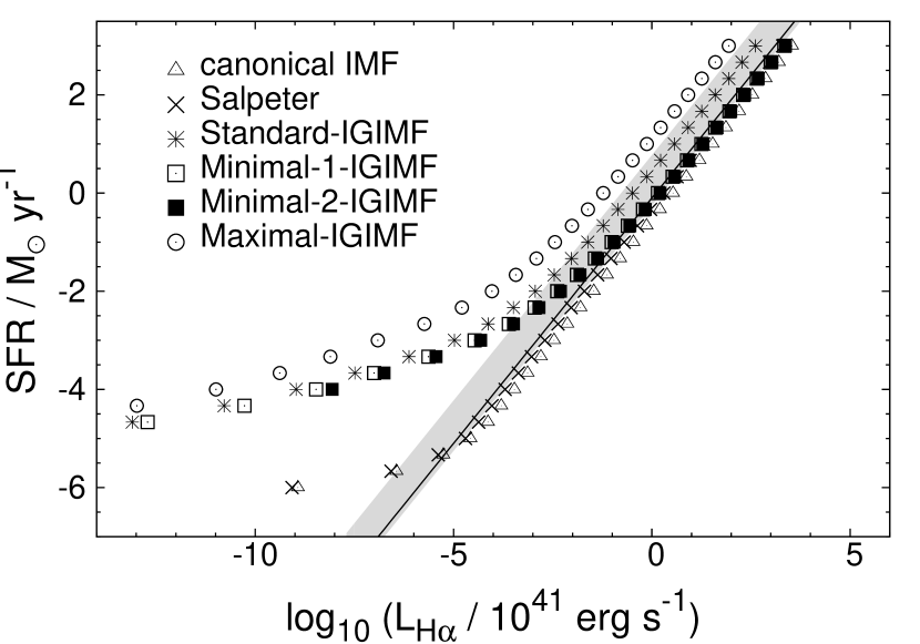
Figure 5: The calculated relation between the SFR and the resulting H$\alpha$-luminosity for four different IGIMF-models and two invariant models in which the IGIMF is assumed to be the canonical IMF and the Salpeter IMF. The solid line represents the widely used linear relation, Eq. 14, by Kennicutt et al. (1994). The gray shaded area marks the full set of linear $L_{\mathrm{H}\alpha}$-SFR relations (Kennicutt et al., 1994) combining different stellar evolution models and different IMFs (for details see text).

The IGIMF models are nearly linear above an H$\alpha$ luminosity of about 10⁴⁰ erg s^-1, which is the lower value of the normal disk galaxies explored by Kennicutt (1983), whereas the relations become much flatter below 10⁴⁰ erg s^-1. As expected the IGIMF-models lie above the linear relations. The order of magnitude of the deviation of the IGIMF-$L_{\mathrm{H}\alpha}$-SFR relation from the linear $L_{\mathrm{H}\alpha}$-SFR relation is independent of the explicit choice of the IGIMF model.

For high $H\alpha$ luminosities our invariant models are strongly linear like the Kennicutt relations. Below a SFR of about 10^-5 M_⊙ yr^-1 they become shallower. In our invariant model the IGIMF is replaced by the canonical IMF. But the IMF is normalised such that the total mass contained in it is still given by

$$\mathrm{SFR}\;\delta t=\int_{m_{\mathrm{min}}}^{m_{\mathrm{max}}}m\;\xi(m)\;\mathrm{dm}\;\;\;,$$ (15)

where $m_{\mathrm{max}}$ is the minimum of the physical upper mass limit, $m_{\mathrm{max*}}$ and the total mass content, $\mathrm{SFR}\;\delta t$ (a star cannot be more massive than the total mass out of which it is formed). Note that $\xi(m)=\xi_{\mathrm{Mecl}}(m)$ (Eq. 9) for $m_{\mathrm{max}}=m_{\mathrm{max*}}$. If the mass available for star formation within the epoch $\delta t$ is less than the physical upper mass limit $m_{\mathrm{max*}}$ then the upper limit of the IMF is given by the amount of available mass. Thus, at a SFR of

$$\mathrm{SFR}=\frac{m_{\mathrm{max*}}}{\delta t}=\frac{150\;\mathrm{M}_{\odot}}{10\;\mathrm{Myr}}=10^{-4.82}\;\frac{\mathrm{M}_{\odot}}{\mathrm{yr}}$$ (16)

our $L_{\mathrm{H\alpha}}$-SFR relations diverge from linearity. The simple physical boundary condition that stars more massive the $SFR\;\delta t$ cannot form leads to non-linear behaviour of the $L_{\mathrm{H\alpha}}$-SFR relation.

For dwarf irregular galaxies having H$\alpha$ luminosities between 10^-36 and 10^-39 erg s^-1 the underestimation of the SFRs vary by a factor of at least 20 to 160 for the Minimal Scenario. In the Maximal Scenario the underestimation of SFRs vary between a factor of 800 and 5000. The SFRs of normal disk galaxies with an H$\alpha$ luminosity of about 10⁴⁰–10⁴² erg s^-1 may be underestimated by a factor of 4 up to 50.

2.5 Fitting functions

For convenient use of the obtained $L_{\mathrm{H}\alpha}$-SFR relation we provide fitting functions for each IGIMF-model. The general form of the fitting function is a polynomial of fifth-order,

$$y=a_{5}x^{5}+a_{4}x^{4}+a_{3}x^{3}+a_{2}x^{2}+a_{1}x+a_{0}\;\;\;.$$ (17)

This function is used to fit the data-points of each IGIMF-model (Fig. 5). The argument and the function value of the fitting-function are

$$x=\log_{10}\left(L_{\mathrm{H}\alpha}\left[10^{41}\mathrm{erg}\;\mathrm{s}^{-1}\right]\right)\;\;\;,$$

$$f(x)=\log_{10}\left(\mathrm{SFR}\left[\mathrm{M}_{\odot}\;\mathrm{yr}^{-1}\right]\right)\;\;\;.$$ (18)

The obtained values of the fitting parameters are listed in Tab. 2 for each model and the fitted models are plotted in Fig. 6.

Table 2: List of the fitting parameters of the $L_{\mathrm{H}\alpha}$-SFR relation

							$L_{\mathrm{H}\alpha}$-range
Model	$a_{5}$	$a_{4}$	$a_{3}$	$a_{2}$	$a_{1}$	$a_{0}$	(erg s-1)
Standard	-2.67e-05	-9.30e-04	-8.47e-03	+3.21e-02	+9.64e-01	+4.38e-01	$1.7\cdot 10^{25}$ – $4.1\cdot 10^{43}$
Maximal	-2.94e-05	-9.97e-04	-9.13e-03	+2.67e-02	+9.63e-01	+1.11e-00	$7.4\cdot 10^{25}$ – $1.2\cdot 10^{43}$
Minimal-1	-2.32e-05	-7.51e-04	-5.70e-03	+4.23e-02	+8.85e-01	-1.58e-01	$3.1\cdot 10^{25}$ – $2.2\cdot 10^{44}$
Minimal-2	3.84e-05	-2.43e-04	-6.58e-03	+3.50e-02	+8.94e-01	-1.91e-01	$8.6\cdot 10^{32}$ – $2.3\cdot 10^{44}$

Note. — Fit-parameters of the fitting-function (Eq. 17) for the four different IGIMF-models: Standard, Maximal, Minimal-1 and Minimal-2 and the luminosity range of data points used for the fit.

Figure 6: Fitted plot of the four IGIMF $L_{\mathrm{H}\alpha}$-SFR relations (crosses) using the fit function Eq. 17 and the parameters of Tab. 2 (solid lines).

The linear parts of our invariant models can be described by

$$\mathrm{SFR}=\frac{L_{\mathrm{H}\alpha}}{1.89\cdot 10^{41}\;\mathrm{erg}\;\mathrm{s}^{-1}}\;\mathrm{M}_{\odot}\;\mathrm{yr}^{-1}\;\;,$$

$$\mathrm{for}\;\;\;L_{\mathrm{H}\alpha}\geq 2.8\cdot 10^{36}\;\mathrm{erg}\;\mathrm{s}^{-1}$$ (19)

in the case of the canonical IMF and

$$\mathrm{SFR}=\frac{L_{\mathrm{H}\alpha}}{3.3\cdot 10^{41}\;\mathrm{erg}\;\mathrm{s}^{-1}}\;\mathrm{M}_{\odot}\;\mathrm{yr}^{-1}\;\;,$$

$$\mathrm{for}\;\;\;L_{\mathrm{H}\alpha}\geq 4.9\cdot 10^{36}\;\mathrm{erg}\;\mathrm{s}^{-1}$$ (20)

in the case of the Salpeter- IMF.

3 SFRs of dIrr

To study the effect of the IGIMF in real systems we now calculate the SFRs of the Sculptur dwarf irregular galaxies. The H$\alpha$ luminosities are taken from Skillman et al. (2003) and are already corrected for galactic extinction but not for N ii contamination as these dwarf galaxies have typically very low nitrogen abundances. The SFRs are obtained using the fitting function Eq. (17). The SFRs in Skillman et al. (2003) are based on the classical relation Eq. 14.

Observed H$\alpha$ luminosities, linear and IGIMF-SFRs and H i masses, $M_{\mathrm{HI}}$ , for eleven Sculptor dwarf irregular galaxies are listed in Tab. 3. The relation between the total galaxy gas mass, $M_{\mathrm{gas}}$, and the SFR can be seen in Fig. 7. To account for Helium the total galaxy gas masses are calculated from

$$M_{\mathrm{gas}}=1.32\;M_{\mathrm{HI}}\;\;\;,$$ (21)

following Skillman et al. (2003).

The conventional data based on the Kennicutt relation (asterisks in Fig. 7) can be divided roughly into two parts. Above a galaxy gas mass of about $2\cdot 10^{7}$ M_⊙ the SFRs are uniformly distributed around a value of about $7\cdot 10^{-3}$ M_⊙ yr^-1 with a large scatter ranging from $2.8\cdot 10^{-4}$ to $5.0\cdot 10^{-2}$ M_⊙ yr^-1. Below a galaxy gas mass of about $2\cdot 10^{7}$ M_⊙ there is a steep decline of the SFR with decreasing galaxy gas mass. This relation is changed by the standard-IGIMF-effect (filled squares) in three ways: Firstly, all SFRs are increased. This increase is larger for low SFRs and therefore mainly for small galaxy gas masses. Secondly, the scatter of SFRs above a total galaxy gas mass of about $2\cdot 10^{7}$ M_⊙ reduces by about one order of magnitude. Thirdly, the decrease of the SFR with decreasing total galaxy gas mass becomes less steep.

A bivariate linear regression between the SFRs derived in the Standard-IGIMF model and the total galaxy gas mass (Fig. 7, solid line) leads to the relation

$$\log_{10}\frac{SFR}{\mathrm{M}_{\odot}\;\mathrm{yr}^{-1}}=1.05\cdot\log_{10}\frac{M_{\mathrm{gas}}}{\mathrm{M}_{\odot}}-10.05\;\;\;.$$ (22)

Figure 7: SFRs in Sculptor dwarf irregular galaxies in dependence of the total galaxy gas mass. The galaxy gas masses and the SFRs calculated using the Kennicutt-relation are taken from Skillman et al. (2003, Tab. 3). These SFRs are compared with the ones obtained using the standard-IGIMF relation (SFR_STD values in Tab. 2) and with our invariant model where the IGIMF is replaced by a canonical IMF. The solid line marks the bivariate regression to the data calculated with the Standard-IGIMF described by Eq. 22.

This means that the SFRs of the Sculptor dwarf irregular galaxies depends linearly on the total gas mass:

$$SFR=8.9\cdot 10^{-11}\;\frac{\mathrm{M}_{\odot}}{\mathrm{yr}^{-1}}\;\;\cdot M_{\mathrm{gas}}^{1.05}\;\;\;.$$ (23)

The corresponding gas depletion time scales,

$$\tau_{\mathrm{gas}}=M_{\mathrm{gas}}/SFR\;\;\;,$$ (24)

are shown in Fig. 8. While the gas depletion times vary by a factor of 400 in the linear (Kennicutt) picture, the IGIMF leads to a shrinkage of the range down to only a factor of 20. Additionally, the strong increase of the gas depletion time with lower galaxy gas mass disappears and the gas depletion time becomes constant at a few Gyr. This is not surprising, as a strictly linear dependence of the SFR on the total gas mass,

$$SFR=AM_{\mathrm{gas}}\;\;\;,$$ (25)

directly implies a constant gas depletion time scale,

$$\tau_{\mathrm{gas}}=M_{\mathrm{gas}}/SFR=A^{-1}\;\;\;.$$ (26)

Figure 8: Gas depletion times in Sculptor dwarf irregular galaxies in dependence of the total galaxy gas mass. The galaxy gas masses and the SFRs calculated using the $L_{\mathrm{H\alpha}}$-SFR relation by Kennicutt are taken from Skillman et al. (2003, Tab. 3). These SFRs are compared with the ones obtained using the Standard-IGIMF $L_{\mathrm{H\alpha}}$-SFR relation (Tab. 2).

Table 3: SFRs of Sculptor dIrr Galaxies

	$M_{\mathrm{H{\sc I}}}$	$\log_{10}(L_{\mathrm{H}\alpha})$	SFRSkill	SFRSTD	SFRMIN1	SFRMIN2	SFRMAX
Galaxy	(106 M⊙)	(erg s-1)	(M⊙ yr-1)	(M⊙ yr-1)	(M⊙ yr-1)	(M⊙ yr-1)	(M⊙ yr-1)
ESO 347-G17	120	38.9	$6.3\cdot\;10^{-3}$	$4.1\cdot\;10^{-2}$	$1.6\cdot\;10^{-2}$	$1.4\cdot\;10^{-2}$	$1.9\cdot\;10^{-1}$
ESO 471-G06	163	38.4	$2.0\cdot\;10^{-3}$	$1.8\cdot\;10^{-2}$	$7.9\cdot\;10^{-3}$	$6.6\cdot\;10^{-3}$	$8.0\cdot\;10^{-2}$
ESO 348-G09	84.3	37.5	$2.8\cdot\;10^{-4}$	$5.0\cdot\;10^{-3}$	$2.6\cdot\;10^{-3}$	$2.2\cdot\;10^{-3}$	$2.1\cdot\;10^{-2}$
SC 18	5.0	36.5	$2.4\cdot\;10^{-5}$	$1.5\cdot\;10^{-3}$	$9.3\cdot\;10^{-4}$	$8.4\cdot\;10^{-4}$	$6.2\cdot\;10^{-3}$
NGC59	16.7	38.6	$3.1\cdot\;10^{-3}$	$2.5\cdot\;10^{-2}$	$1.0\cdot\;10^{-2}$	$8.8\cdot\;10^{-3}$	$1.1\cdot\;10^{-1}$
ESO 473-G24	63.8	38.2	$1.3\cdot\;10^{-3}$	$1.3\cdot\;10^{-2}$	$6.0\cdot\;10^{-3}$	$5.0\cdot\;10^{-3}$	$5.8\cdot\;10^{-2}$
SC 24	2.1	35.4	$2.1\cdot\;10^{-6}$	$5.8\cdot\;10^{-4}$	$4.0\cdot\;10^{-4}$	$4.0\cdot\;10^{-4}$	$2.2\cdot\;10^{-3}$
DDO226	33.9	38.2	$1.3\cdot\;10^{-3}$	$1.3\cdot\;10^{-2}$	$6.0\cdot\;10^{-3}$	$5.0\cdot\;10^{-3}$	$5.8\cdot\;10^{-2}$
DDO6	15.4	37.6	$2.9\cdot\;10^{-4}$	$5.7\cdot\;10^{-3}$	$2.9\cdot\;10^{-3}$	$2.4\cdot\;10^{-3}$	$2.4\cdot\;10^{-2}$
NGC 625	118	39.8	$5.0\cdot\;10^{-2}$	$2.2\cdot\;10^{-1}$	$7.1\cdot\;10^{-2}$	$6.3\cdot\;10^{-2}$	$1.0\cdot\;10^{-0}$
ESO 245-G05	289	39.1	$1.0\cdot\;10^{-2}$	$5.9\cdot\;10^{-2}$	$2.2\cdot\;10^{-2}$	$1.9\cdot\;10^{-2}$	$2.7\cdot\;10^{-1}$

Note. — Integrated H$\alpha$ luminosities and determined SFRs by Skillman et al. (2003) using the Kennicutt-relation (Eq. 14). The SFRs of the dIrrs for the IGIMF-models are calculated using our fitting functions.

4 H$\alpha$-invisible SF

The determination of the SFR of a galaxy is based on the measurement of a total H$\alpha$ luminosity of the galaxy and a reliable theoretical relation between the current SFR and the produced H$\alpha$ radiation. The H$\alpha$ emission is confined within distinct H ii-regions. These regions have to be identified manually after H$\alpha$ imaging. The emission of these H$\alpha$ regions have to exceed some detection limit to be distinguishable from background radiation and noise and to be detectable.

Assuming that SF takes place in star clusters distributed according to an ECMF with star cluster masses down to a few solar masses then the least luminous observed H ii region is not the smallest star cluster but the cluster producing the lowest observable H$\alpha$ radiation. Thus, the lowest observed H$\alpha$ flux indicates the detection limit. In the work by Skillman et al. (2003) this detection limit is about $4\cdot 10^{-16}$ erg cm^-2 s^-1 (H ii region ESO 348-G9 No.2). In the work by Miller & Hodge (1994) the lowest measured H$\alpha$ flux in M81 group dwarf galaxies is about $6.5\cdot 10^{-16}$ erg cm^-2 s^-1 (IC 2574 MH 135). Assuming that each star cluster forms its own H ii region created by all ionising stars formed in this star cluster, a mass-luminosity relation (Fig. 9) between the embedded star cluster mass and the averaged produced H$\alpha$ luminosity within the star formation epoch $\delta t$ can be constructed as described in Sec. 2.2. This can be well approximated by

$$y=(x+34.55)\;(1-1/\exp(0.27x^{2}+0.46x+0.32))\;\;\;,$$ (27)

with $y=\log_{10}(L_{\mathrm{H}\alpha}/\mathrm{erg\;s}^{-1})$ and $x=\log_{10}(M_{\mathrm{ecl}}/\mathrm{M}_{\odot})$. For comparison the Orion Nebula cluster with a total mass of about 1800 M_⊙ (Hillenbrand & Hartmann, 1998) and an observed H$\alpha$ luminosity of 10³⁷ erg s^-1 (Kennicutt, 1984) and 30 Doradus with a total mass of about 272000 M_⊙ (Selman et al., 1999) and an observed H$\alpha$ luminosity of $1.5\cdot 10^{40}$ erg s^-1 (Kennicutt, 1984) are marked, lying well on the mass-H$\alpha$ luminosity relation.

The Sculptor dwarf irregular galaxy SC 24, for example, has only one observable H ii-region. Its flux is $8\cdot 10^{-15}$ erg cm^-2 s^-1 (Skillman et al., 2003) being just above the detection limit. Given the distance of SC 24 of about 2.14 Mpc the H$\alpha$ luminosity of the most luminous H ii-region in SC 24 is $2.5\cdot 10^{35}$ erg s^-1. Given our mass-luminosity relation (Fig. 9) the corresponding star cluster stellar mass is about 280 M_⊙. Eq. 4 then determines the current SFR to be about $5.0\cdot 10^{-4}$ M_⊙ yr^-1 in good agreement with the Standard-IGIMF Scenario rather than the classical one (Tab. 3). The classical SFR of $2.1\cdot 10^{-6}$ M_⊙ yr^-1 implies that only 1 M_⊙ of stellar material will have formed within 1 Myr which is by two orders of magnitude inconsistent with the expected cluster mass (280 M_⊙). However, our SFR of $5.8\cdot 10^{-4}$ means that 580 M_⊙ must have formed within 1 Myr showing an internal consistency of our picture.

Figure 9: Mass-luminosity relation between the stellar mass of the cluster and the produced total H$\alpha$ emission. The solid line shows the fit by Eq. 27. The observed position of the Orion Nebula cluster and 30 Doradus are indicated for comparison. Note the steep decline of $L_{\mathrm{H\alpha}}$ for $M_{\mathrm{ecl}}\lesssim$ 1000 M_⊙ is a result of the $m_{\mathrm{max}}(M_{\mathrm{ecl}})$ relation (Fig. 1).

Figure 10: Relation between the stellar mass of embedded star clusters and the maximum distance of the star cluster within which the star cluster can be detected with H$\alpha$ observations in the case of three different detection limits: 10^-15, 10^-16 and 10^-17 erg s^-1 cm^-2.

An H ii-region with the luminosity L_Hα in a galaxy at a distance $D$ produces an H$\alpha$ flux of

$$j=\frac{L_{\mathrm{H}\alpha}}{4\pi D^{2}}\;\;\;.$$ (28)

Using the mass-H$\alpha$ luminosity relation (Eq. 27) and a detection limit, $j_{\mathrm{limit}}$, a relation between the star cluster mass and the maximum distance, $D_{\mathrm{max}}$, within which the star cluster can be observed, can be constructed (Fig. 10).

If the Sculptor dwarf galaxy SC 24 were located more distant than 2.3 Mpc then SF in SC 24 would not have been detected. Therefore very moderate SF can be overseen. The effect of H$\alpha$-dark star formation on the cosmological SFR due to a possible large number of dwarf galaxies with low SFRs needs further study.

5 Conclusion

Using the integrated galaxial initial mass function (IGIMF) instead of an invariant IMF for calculating the produced H$\alpha$-luminosity for a given galaxy-wide SFR we revise the linear $L_{\mathrm{H}\alpha}$-SFR relation by Kennicutt et al. (1994). The order of magnitude of the deviation of the IGIMF-$L_{\mathrm{H}\alpha}$-SFR relation from the linear $L_{\mathrm{H}\alpha}$-SFR relation is independent of the explicit choice of the IGIMF model.

Because the fraction of massive stars determined by the IGIMF is always less than given by the underlying invariant IMF of individual star clusters, SFRs are always underestimated when using linear $L_{\mathrm{H\alpha}}$-SFR relations. The linearity between the H$\alpha$ luminosity and the SFR is broken, too. Therefore, the SFRs of normal disk galaxies with an H$\alpha$ luminosity of about 10⁴⁰–10⁴² erg s^-1 may be underestimated by a factor of 4 up to 50. For dwarf irregular galaxies having H$\alpha$ luminosities between 10^-36 and 10^-39 erg s^-1 the underestimation of the SFRs vary by a factor of at least 20 to 160 for the Minimal Scenario. In the Maximal Scenario the underestimation of SFRs of dwarf galaxies vary between a factor of 800 and 5000. Evolutionary parameters of dwarf galaxies such as the gas depletion time scale are effected by the same order of magnitude. In fact, we find the IGIMF formulation to imply a linear dependence of the total SFR on the total galaxy gas mass and therefore the gas depletion time scale to be constant, a few Gyr, and independent of the total galaxy gas mass.

If this finding is correct it imposes a problem for the theoretical understanding of galactic star formation explaining the apparent low star formation efficiency of small galaxies (e.g. Kaufmann et al., 2007).

Observational evidence confirming the IGIMF scenario is becoming available (Hoversten & Glazebrook, 2007) but further observational work is needed. Additionally, more consistency checks with different methods of deriving SFRs should be done in future.

Further work is required to construct reliable conversions of IGIMF-fluxes into other pass bands. Kennicutt (1998) mentioned that H$\alpha$ measurements become unreliable for determining SFRs in regions with gas densities higher than 100 M_⊙ pc^-2 as present in star burst galaxies. An extension of the IGIMF-model to construct a relation between SFRs and FIR luminosities is therefore clearly necessary.

References

- Bonnell et al. (2004) Bonnell I. A., Vine S. G., Bate M. R., 2004, MNRAS, 349, 735
- Bressan et al. (1993) Bressan A., Fagotto F., Bertelli G., Chiosi C., 1993, A&AS, 100, 647
- Bruzual & Charlot (2003) Bruzual G., Charlot S., 2003, MNRAS, 344, 1000
- Diehl et al. (2006) Diehl R., Halloin H., Kretschmer K., Lichti G. G., Schönfelder V., Strong A. W., von Kienlin A., Wang W., Jean P., Knödlseder J., Roques J.-P., Weidenspointner G., Schanne S., Hartmann D. H., Winkler C., Wunderer C., 2006, Nature, 439, 45
- Figer (2005) Figer D. F., 2005, Nature, 434, 192
- Hillenbrand & Hartmann (1998) Hillenbrand L. A., Hartmann L. W., 1998, ApJ, 492, 540
- Hoversten & Glazebrook (2007) Hoversten E., Glazebrook K., 2007, ApJ, submitted (preprint)
- Hurley et al. (2000) Hurley J. R., Pols O. R., Tout C. A., 2000, MNRAS, 315, 543
- Kaufmann et al. (2007) Kaufmann T., Wheeler C., Bullock J. S., 2007, ArXiv e-prints, 706
- Kennicutt (1983) Kennicutt Jr. R. C., 1983, ApJ, 272, 54
- Kennicutt (1984) Kennicutt Jr. R. C., 1984, ApJ, 287, 116
- Kennicutt (1998) Kennicutt Jr. R. C., 1998, ApJ, 498, 541
- Kennicutt et al. (1994) Kennicutt Jr. R. C., Tamblyn P., Congdon C. E., 1994, ApJ, 435, 22
- Koen (2006) Koen C., 2006, MNRAS, 365, 590
- Köppen et al. (2007) Köppen J., Weidner C., Kroupa P., 2007, MNRAS, 375, 673
- Kroupa (2001) Kroupa P., 2001, MNRAS, 322, 231
- Kroupa (2002) Kroupa P., 2002, Science, 295, 82
- Kroupa et al. (1993) Kroupa P., Tout C. A., Gilmore G., 1993, MNRAS, 262, 545
- Kroupa & Weidner (2003) Kroupa P., Weidner C., 2003, ApJ, 598, 1076
- Larsen (2000) Larsen S. S., 2000, MNRAS, 319, 893
- Larsen (2002a) Larsen S. S., 2002a, in Geisler D., Grebel E. K., Minniti D., eds, IAU Symposium Open, Massive and Globular Clusters – Part of the Same Family?. pp 421–+
- Larsen (2002b) Larsen S. S., 2002b, AJ, 124, 1393
- Larsen & Richtler (2000) Larsen S. S., Richtler T., 2000, A&A, 354, 836
- Lee et al. (2004) Lee H.-c., Gibson B. K., Flynn C., Kawata D., Beasley M. A., 2004, MNRAS, 353, 113
- Lejeune et al. (1997) Lejeune T., Cuisinier F., Buser R., 1997, A&AS, 125, 229
- Lejeune et al. (1998) Lejeune T., Cuisinier F., Buser R., 1998, A&AS, 130, 65
- Maíz Apellániz et al. (2006) Maíz Apellániz J., Walborn N. R., Morrell N. I., Niemela V. S., Nelan E. P., 2006, ArXiv Astrophysics e-prints
- Maschberger & Kroupa (2007) Maschberger T., Kroupa P., 2007, MNRAS, 379, 34
- McKee & Williams (1997) McKee C. F., Williams J. P., 1997, ApJ, 476, 144
- Meynet & Maeder (2003) Meynet G., Maeder A., 2003, A&A, 404, 975
- Miller & Hodge (1994) Miller B. W., Hodge P., 1994, ApJ, 427, 656
- Oey & Clarke (2005) Oey M. S., Clarke C. J., 2005, ApJ, 620, L43
- Pflamm-Altenburg & Kroupa (2006) Pflamm-Altenburg J., Kroupa P., 2006, MNRAS, 373, 295
- Scalo (1986) Scalo J. M., 1986, Fundamentals of Cosmic Physics, 11, 1
- Schaller et al. (1992) Schaller G., Schaerer D., Meynet G., Maeder A., 1992, A&AS, 96, 269
- Selman et al. (1999) Selman F., Melnick J., Bosch G., Terlevich R., 1999, A&A, 347, 532
- Selman & Melnick (2005) Selman F. J., Melnick J., 2005, A&A, 443, 851
- Skillman et al. (2003) Skillman E. D., Côté S., Miller B. W., 2003, AJ, 125, 593
- Stahler & Palla (2005) Stahler S. W., Palla F., 2005, The Formation of Stars. The Formation of Stars, by Steven W. Stahler, Francesco Palla, pp. 865. ISBN 3-527-40559-3. Wiley-VCH , January 2005.
- Vanbeveren (1982) Vanbeveren D., 1982, A&A, 115, 65
- Vanbeveren (1983) Vanbeveren D., 1983, A&A, 124, 71
- Weidner & Kroupa (2004) Weidner C., Kroupa P., 2004, MNRAS, 348, 187
- Weidner & Kroupa (2005) Weidner C., Kroupa P., 2005, ApJ, 625, 754
- Weidner & Kroupa (2006) Weidner C., Kroupa P., 2006, MNRAS, 365, 1333
- Weidner et al. (2004) Weidner C., Kroupa P., Larsen S. S., 2004, MNRAS, 350, 1503
- Westera et al. (2002) Westera P., Lejeune T., Buser R., Cuisinier F., Bruzual G., 2002, A&A, 381, 524