The Star Formation Law in a Multifractal ISM

Abstract

The surface density of the star formation rate in different galaxies, as well as in different parts of a single galaxy, scales nonlinearly with the surface density of the total gas. This observationally established relation is known as the Kennicutt-Schmidt star formation law. The slope of the star formation law has been shown to change with the density of the gas against which the star formation rate is plotted. This dependence implies a nonlinear scaling between the dense gas and the total gas surface densities within galaxies. Here, we explore a possible interpretation of this scaling as a property of the geometry of the interstellar medium (ISM), and we find that it arises naturally if the topology of the ISM is multifractal. Under the additional assumption that, at very high densities, the star formation timescale is roughly constant, the star formation law itself can also be recovered as a consequence of the multifractal geometry of the ISM. The slope of the scaling depends on the width of the global probability density function (PDF), and is between $1.5$ and $1.6$ for wide PDFs relevant to high-mass systems, while it is higher for narrower PDFs appropriate for lower-mass dwarf galaxies, in agreement with observations.

1 Introduction

The dependence of the star formation rate on gas density on large scales is a subject of intense observational and theoretical investigation, as it is both an important input for models of galaxy formation and evolution and chemical evolution calculations, as well as a critical test for theories of interstellar medium evolution and star formation. Let us define the surface density of the star formation rate, $\dot{\Sigma}_{\rm SF}$, as the mass of gas being converted into stars per unit time per unit surface area, and $\Sigma_{\rm gas}$ as the total gas mass per unit surface area. The two quantities have been found to obey a non-linear, power-law relation:

$$\dot{\Sigma}_{\rm SF}\propto\Sigma_{\rm gas}^{n_{\rm gas}}\,,$$ (1)

where $n_{\rm gas}\approx 1.5$ for a large range of surface densities and system morphologies. This correlation is known as the Kennicutt-Schmidt law of star formation (Schmidt 1959, Kennicutt 1989). The star formation law has been established through observations of the global star formation and gas density in different galaxies (e.g. Kennicutt 1998, Misiriotis et al. 2004, Komugi et al. 2005); of local gas and star formation densities in different galaxies (e.g. Wong and Blitz 2002, Boissier et al 2003); and of local gas and star formation densities within a single galaxy (e.g. Misiriotis et al. 2006 in the case of the Milky Way, Schuster et al. 2007 in the case of M51).

Traditionally, this correlation has been interpreted in the literature as a result of the density dependence of the star-formation timescale. The star formation rate density can be expressed as a ratio of the density of the gas available for star formation over a timescale relevant to the conversion of the available gas to stars. Examples of such timescales that have been suggested in this framework are the free-fall timescale, the turbulence crossing time over the scale height of the galaxy, the collapse timescale of large expanding shells with low Mach number (see e.g. Elmegreen 2002b and references therein), the orbital timescale of the galactic disk (Silk 1997), and the timescale for gas accumulation along magnetic flux tubes parallel to spiral arms, into the valleys created by the magnetic Rayleigh-Taylor (Parker) instability (see e.g. Shu et al. 2007). These timescales all scale as the inverse square root of density, resulting in an overall scaling of the star formation density as gas density to the $1.5$. A more elaborate treatment based on the same principle was presented by Krumholz and McKee (2005). This interpretation of the star formation law is very tempting because it is conceptually simple and elegant, and because it gives the same result for several different processes which may be controlling the star formation timescale. However, a series of more recent observations have indicated that this simple picture may not be a complete interpretation of the star formation law.

First of all, the value $n_{\rm gas}\approx 1.5$, although consistent with observations of a large range of star-forming systems, is by no means unique. Appreciable scatter exists that cannot be entirely attributed to observational uncertainties and cannot be comfortably reconciled with a theoretically set single value of $n_{\rm gas}$. For example, if only gas with local volume densities representative of molecular cloud cores is included in the gas surface density (as is the case when tracers sensitive to higher density gas are used, such as HCN) the resulting scaling is closer to linear,

$$\dot{\Sigma}_{\rm SF}\propto\Sigma_{\rm den,gas}^{n_{\rm dense}}\,,$$ (2)

where $\Sigma_{\rm den,gas}$ is the surface density of the denser gas, and $n_{\rm dense}$ is now closer to $1$ rather than $1.5$ (e.g. Gao and Solomon 2004, Wu et al. 2005). Observations of dwarf galaxies on the other hand seem to favor much steeper scalings (values of $n_{\rm gas}$ much larger than $1.5$). For example, de Blok and Walter (2006) find for NGC 6822 a slope 2.04; Heyer et al. (2004) find for M33 a much steeper slope, equal to 3.3; in the case of IC10, Leroy et al. (2006), find a slope of $1.4$ for molecular gas and a slope much steeper than $1.5$ for the total gas density (see their Fig. 14).

In addition, since star formation is an inherently local phenomenon, the connection between the small scales ($\sim 0.1{\rm\,pc}$) where stars form, and the large scales ($\sim 1{\rm\,kpc}$) that the gas density observations and the associated timescales refer to, may be quite complicated. The traditional interpretation implicitly assumes that a meaningful mean density can be assigned to the large scales where $\Sigma_{\rm gas}$ is determined. However, this need not be the case. As a counter-example, we can consider the situation where several dense objects are sparsely distributed over a region of $\sim{\rm\,kpc}$ dimensions. The mean density we would derive would be rather low, but it would not be representative of any object in the region. Consequently, the star-formation timescale calculated at that mean density would not represent the real timescale over which any of the objects in the region evolve. Instead, the relevant timescale for star formation should be constructed out of the densities of the individual star-forming sites rather than the large-scale mean density.

Finally, the interstellar medium (ISM) is a highly complex system, and its structure and properties are the result of a synthesis of nonlinear phenomena and instabilities, not necessarily connected with one another. Star formation on the other hand only occurs at the density peaks of the ISM, and it is likely that the star formation law may be conveying information about the connection between the large-scale low-density ISM and its small-scale high-density peaks, rather than information about the star formation process itself.

The connection between the high-density and low-density ISM gas is imprinted in different incarnations of the star formation law. Observations have established that the slope of the scaling of the star formation rate surface density with the gas surface density depends on the minimum density of the gas accounted for in observations [Eqs. (1) and (2)]. If now we demand that Eqs. (1) and (2) both hold, this implies a scaling between the surface densities of total gas and dense gas,

$$\Sigma_{\rm den,gas}\propto\Sigma_{\rm gas}^{n}\,,$$ (3)

with $n=n_{\rm gas}/n_{\rm dense}\approx n_{\rm gas}\approx 1.5$.

In this paper we investigate this connection, and we examine the extent to which such a nonlinear scaling of the dense gas surface density with the total gas surface density can be interpreted as a topological property of the ISM. In particular, we investigate whether such a scaling can arise naturally in multifractal topologies.

While fractal structures are characterized by a unique non-integer generalized dimension, a spectrum of generalized fractal dimensions is required to fully describe multifractal structures. In a multifractal structure, we can define a scaling exponent which characterizes the structure locally, around each point. Sets of points that share the same scaling exponent constitute a fractal. The distribution of fractal dimensions of all such fractals is the multifractal spectrum, which describes the distribution of geometries present in a complex structure.

The gas and dust in the ISM is organized in complicated structures with irregularities present over a wide range of scales. Different studies have used different techniques to quantify the properties of these structures and describe the geometry of the ISM: e.g., autocorrelation function (Dickman and Kleiner 1985), power spectra (Stützki et al. 1998); perimeter/area relation (Bazell and Desert 1988; Scalo 1990; Vogelaar and Wakker 1994; Westpfahl et al. 1999 in HI for members of the M81 group), wavelet analysis (Langer et al. 1993), principal component analysis (Heyer and Schloerb 1997), multifractal scaling (Chappell and Scalo 2001). These studies find that structure in the ISM has a scale-free, hierarchical appearance. This complexity over a wide range of scales has lead to the proposition that a multifractal ISM geometry with a lognormal probability density function (PDF) is consistent with many of the observed features, including the mass and size distribution of clouds and the ISM filling factor (Elmegreen 2002a; Elmegreen et al. 2006). The physics is usually associated with compressible turbulence (e.g., Mac Low and Klessen 2004, Scalo and Elmegreen 2004), however the multifractal scaling is much more generic and may arise from many different multiplicative hierarchical processes (e.g. Colombi, Bouchet, and Schaeffer 1992; Sylos Labini and Pietronero 1996).

It should be noted that the ISM cannot be strictly scale-free, since optical observations of a variety of galaxies suggest an upper characteristic scale ($\sim$1 kpc) that can either be the Jeans length (e.g. Elmegreen 2004) or the wavelength of the Parker instability (Mouschovias, Shu and Woodward 1974). A lower characteristic scale also exists, at the order of $\sim$0.1 pc (Blitz and Williams 1997; Barranco and Goodman 1998; Goodman et al. 1998). However, in between these scales, a variety of different processes and instabilities can lead to multifractal scalings and lognormal PDFs (e.g. Vazquez-Semadeni 1994; Kravtsov 2003; Wada & Norman 2007).

The purpose of this work is to examine whether a nonlinear scaling of the dense gas surface density with the total gas surface density similar to that of Eq. (3) can arise naturally in multifractal ISM geometries, whether it is robust enough to resemble the persistence and uniformity of $n_{\rm gas}/n_{\rm dense}$ over a variety of star forming systems with different local conditions, and whether it can allow for different slopes seen e.g. in observations of dwarf galaxies under physical conditions similar to those found in these systems.

A geometrical explanation to Eq. (3) has an additional tantalizing potential consequence. Equation (2) implies that the star formation rate surface density scales linearly with the very dense gas, or, equivalently, that at those high densities the star formation timescale is roughly constant and independent of $\Sigma_{\rm den,gas}$:

$$\dot{\Sigma}_{\rm SF}=\frac{\Sigma_{\rm den,gas}}{\tau_{\rm SF,dense}}$$ (4)

with $\tau_{\rm SF,dense}\sim{\rm const}$. However, in this case $\dot{\Sigma}_{\rm SF}\propto\Sigma_{\rm den,gas}$ and if $\Sigma_{\rm gas}\propto\Sigma_{\rm den,gas}^{n}$ due to geometry, then $\dot{\Sigma}_{\rm SF}\propto\Sigma_{\rm gas}^{n}$. The observationally motivated assumption of a star formation timescale independent of $\Sigma_{\rm den}$ at high densities, in combination with a topologically-driven scaling between dense and total gas, can thus provide a geometrical interpretation of the star formation law itself.

This paper is structured as follows. Our formulation and our algorithms for the reproduction of multifractal three-dimensional geometries are discussed in Section 2. Our results are presented in Section 3. We discuss our findings in Section 4, and we summarize our conclusions in Section 5.

2 Formulation

In order to investigate how the mean surface density of very dense gas correlates with the surface density of the total gas in different multifractal ISM topologies, we need to generate a multifractal structure, and perform appropriate “observations” of its total and dense “gas” surface densities. In this section, we describe these procedures.

To generate a multi-fractal, we adapt the algorithm of Borgani et al. (1993), which is a modification of the $\beta$ model (Frisch et al. 1978) and the random-$\beta$ model (Benzi et al. 1984) of fully developed turbulence. We start with a parent three-dimensional cube of side $L$, which we divide into $2^{3}$ equal-volume subcubes, each of which inherits some fraction $f_{i}$ of the parent-cube mass, where $i=1,..,8$. Mass conservation implies that $\sum_{i=1}^{8}f_{i}=1$. We repeat the fragmentation (where each subcube now becomes a parent-cube) $H$ times. The fraction of the total mass contained in each final cube of volume $L^{3}/2^{3H}$ depends on its fragmentation history.

The properties of the final structure depend on the choice of $f_{i}$. If all $f_{i}$ are non-zero and equal, then the result is a homogeneous structure. If some of the $f_{i}$ are zero and all of the non-vanishing $f_{i}$ are equal, then the result is a monofractal structure, with a fractal dimension uniquely set by the choice of $f_{i}$. If the non-vanishing $f_{i}$ are not equal, then a multi-fractal structure results. To obtain a pattern-free structure that still retains the scaling properties of a fractal (self-similarity) or a multifractal (self-affinity), the pattern of $f_{i}$ is not kept constant in all iterations: each $f_{i}$ value is assigned to a random subcube $i$ in each iteration.

Each multifractal cube is taken to represent one ISM topology. We investigate how the total gas surface density correlates with the dense gas surface density in different parts of this object in the following way: once a multifractal cube is constructed according to the algorithm above, a line-of-sight is selected, parallel to one side of the cube. The face of the cube which is perpendicular to that line is then split into $2^{2(H-3)}$ square patches (each side of the face is split into $2^{H-3}$ segments). For each of these patches, an “observation” is made of its total surface density, by summing up all of the mass within the volume defined by the patch and extending along the line of sight, and dividing by the surface area of the patch. Similarly, the “dense gas” surface density is calculated by summing up all of the mass within regions of local volume density above the “dense gas” threshold within the same volume, and dividing by the surface area of the patch.

To test the robustness of our results against variations of the detailed properties of the multifractal cube, we have repeated our measurements for seven distinct multifractals. The properties of these multifractals ($f_{i}$ and number of refinement levels, $H$) are given in Table 1.

Table 1: Mass fractions $f_{i}$ and levels of refinement $H$ for the seven multifractals investigated in our study. Multifractals are listed here in order of decreasing PDF width (see Fig. 3).

	$H$	$f_{1}$	$f_{2}$	$f_{3}$	$f_{4}$	$f_{5}$	$f_{6}$	$f_{7}$	$f_{8}$
A	$7$	$0.6$	$0.2$	$0.1$	$0.05$	$0.04$	$0.005$	$0.004$	$0.001$
B	$6$	$0.6$	$0.1$	$0.1$	$0.1$	$0.09$	$0.005$	$0.004$	$0.001$
C	$5$	$0.6$	$0.2$	$0.1$	$0.05$	$0.04$	$0.005$	$0.004$	$0.001$
D	$6$	$0.44$	$0.17$	$0.1$	$0.1$	$0.1$	$0.05$	$0.03$	$0.01$
E	$6$	$0.4$	$0.15$	$0.1$	$0.1$	$0.1$	$0.05$	$0.05$	$0.05$
F	$7$	$0.3$	$0.1$	$0.1$	$0.1$	$0.1$	$0.1$	$0.1$	$0.1$
G	$6$	$0.3$	$0.15$	$0.1$	$0.1$	$0.1$	$0.1$	$0.1$	$0.05$

3 Results

The first questions we seek to answer are whether the scaling between the very dense gas and total gas in a multifractal medium resembles that of Eq. (3); and whether such a scaling is robust enough against variations in the detailed properties of the multifractal (parameterized in our model by the values of the $f_{i}$ and $H$) so that such a scaling can be viewed as an intrinsic property of multifractal geometries, rather than as a result of fine-tuning of the multifractal model.

We address these questions in Fig. 1, which shows the surface density of dense gas, $\Sigma_{\rm den,gas}$, in this case defined as gas with local volume density at least $3\times 10^{3}$ times the mean volume density, as a function of the surface density of total gas $\Sigma_{\rm gas}$, for three different multifractals (A, B, and C). Each datapoint corresponds to a different patch within the multifractal cube. The three fractals depicted in this figure have different mass fractions, $f_{i}$, however they all have “wide” global PDFs (see upper panel of Fig. 3 and discussion below). In all cases, the scaling between $\Sigma_{\rm gas}$ and $\Sigma_{\rm den,gas}$ is clearly nonlinear (significantly deviates from the linear relation plotted in Fig. 1 with the solid line), and has a scaling slope of $\approx 1.5$.

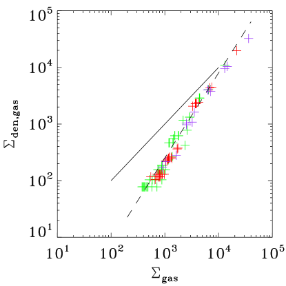
Figure 1: Scaling of dense gas surface density vs. total gas surface density for multifractals A (green), B (red), and C (purple). The solid and dashed lines correspond to the $\Sigma_{\rm den,gas}\propto\Sigma_{\rm gas}$ and $\Sigma_{\rm den,gas}\propto\Sigma_{\rm gas}^{1.5}$ scalings respectively.

To understand the origin of the nonlinearity of the scaling, we need to examine how the gas is distributed over different local densities. This distribution is quantified by the PDF, which is defined as the distribution of volume fraction with respect to local density (where the local density is measured in units of the mean density of the cube). In order to have a nonlinear scaling between the surface densities of total gas and gas density peaks, the PDFs of different patches within the cube must be different from each other. This requirement is straight forward to prove. Let the local PDF within a patch $i$ of volume $V_{i}$ be $g_{i}(\rho)=(1/V_{i})dV/d\rho$. Then, the total dense gas mass in patch $i$ is an integral of the PDF above some high density threshold $\rho_{\rm den}$,

$$M_{\rm den,gas,i}=V_{i}\int_{\rho_{\rm den}}^{\infty}g_{i}(\rho)\rho d\rho\,,$$ (5)

and the total gas mass of the same patch is an integral of the PDF over all densities,

$$M_{\rm gas,i}=V_{i}\int_{0}^{\infty}g_{i}(\rho)\rho d\rho\,,$$ (6)

while the ratio of surface densities is given by

$$\left(\frac{\Sigma_{\rm den,gas}}{\Sigma_{\rm gas}}\right)_{i}=\frac{M_{\rm den,gas,i}/A_{i}}{M_{\rm gas,i}/A_{i}}=\frac{\int_{\rho_{\rm den}}^{\infty}g_{i}(\rho)\rho d\rho}{\int_{0}^{\infty}g_{i}(\rho)\rho d\rho}\,,$$ (7)

where $A_{i}$ is the surface area of the patch perpendicular to the line of sight. If now the PDF remains the same among different patches (all $g_{i}$ are identical), the right-hand side of Eq. (7) is always constant, resulting in an identically linear scaling, $\Sigma_{\rm den,gas}\propto\Sigma_{\rm gas}$. A similar result is obtained, as long as the PDF spread is sufficiently large, if the $g_{i}$ have the same spread but different mean densities. A nonlinear scaling can only arise if different patches exhibit different PDF spreads. This feature is an inherent property of multifractals, as we show below.

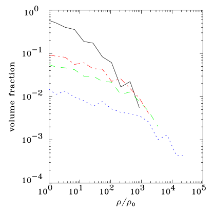
Figure 2: Probability density functions of different patches of multifractal A. The total gas surface density is lowest for the patch represented by the solid black line, and progressively increases for the patches depicted in dashed red, long-dashed green, and dotted blue respectively.

Figure 2 shows local PDFs for four different patches of varying mean density for multifractal A. In our multifractal geometry, the local PDFs are not identical in spread to each other, and they are not identical to the global PDF of the cube (plotted with the thin solid black line in the upper panel of Fig. 3). Instead, they are truncated at different densities depending on their total gas surface density. The total gas surface density is lowest for the patch represented by the solid black line, and progressively increases for the patches depicted in dashed red, long-dashed green, and dotted blue respectively. The lower the total surface density of the patch, the lower the density at which the PDF is truncated. It is this effect which is the origin of the nonlinearity in the scaling of $\Sigma_{\rm den,gas}$ with $\Sigma_{\rm gas}$. A similar dependence of the local PDF on the mean density was pointed out by Kravtsov (2003) in the case of cosmological simulations, where the star formation law was reproduced in large scales, despite the fact that the local star formation recipe featured a timescale constant with density.

We have demonstrated that a nonlinear scaling between very dense and total gas surface densities arises naturally in multifractal geometries, and we have traced its origin in the property of the local multifractal PDF to extend to higher local densities in regions of higher mean density. However, there are still several points to be addressed before we can draw conclusions on how robust this scaling really is, and how it may relate to the star formation law. These points are the following.

1. The definition of “dense gas” we used in our discussion of Fig. 1 was rather arbitrary. We would like to understand how the slope of the scaling may depend on this definition.

2. Although we have shown that different multifractals show similar behaviour, we would like to understand whether scalings with slope other than $\approx 1.5$ can also be recovered, and under what conditions.

3. Although the detailed values of $f_{i}$, together with the number of refinement levels, uniquely determine the multifractal scaling properties, it would be desirable to identify a global property of the multifractal, which controls the slope of the scaling.

4. Finally, we would like to examine whether the conditions under which scalings with slopes different that $\approx 1.5$ appear in our simulated multifractals possibly mirror situations in nature where the $n_{\rm gas}$ slope of the star formation law entering Eq. (3) also has different values (as, for example, in the case of dwarf galaxies).

We address these issues with the help of Figs. 3 and 4.

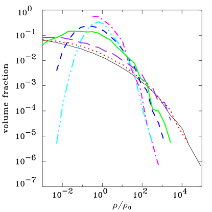
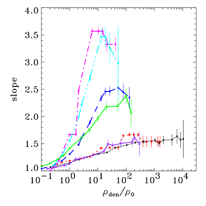
Figure 3: Upper panel: probability density functions for each multifractal. Different line styles and colours correspond to different multifractals as follows: thin solid black $\rightarrow$ A; dotted red $\rightarrow$ B; long-dashed purple $\rightarrow$ C; thick solid green $\rightarrow$ D; dashed blue $\rightarrow$ E; double-dot–dashed cyan $\rightarrow$ F; dot-dashed magenta $\rightarrow$ G. Lower panel: dependence of the exponent $n$ of the scaling between dense gas surface density and total gas surface density on the value of “dense gas” density threshold (in units of the mean density of the multifractal); line styles and colours as in the upper panel.

The upper panel of Fig. 3 shows the PDF of the cube as a whole for each multifractal described in Table 1. The global PDF can be fitted well by a lognormal in all cases. The lower panel of the same figure shows the dependence of the slope $n$ (the scaling between $\Sigma_{\rm den,gas}$ and $\Sigma_{\rm gas}$, see Eq. 3) on the value of the dense gas density threshold, $\rho_{\rm den}$ in units of the mean density of the cube, $\rho_{0}$. The points in the lower panel are generated through fitting power laws to scatter plots similar to those of Fig. 1, where $\Sigma_{\rm den,gas}$ is, in each case, calculated with the appropriate definition of $\rho_{\rm den}$. The error bars in the data points represent the $1\sigma$ uncertainty on the slope of those fits. For higher values of the threshold $\rho_{\rm den}$, fewer points are found within the cube which include mass at such densities, and for this reason the uncertainty on the scaling slope increases. From the two panels of Fig. 3, we can draw the following conclusions.

Figure 4: Dependence of scaling slope $n$ on the definition of $\Sigma_{\rm gas}$. Crosses: scaling of $\Sigma_{\rm den,gas}$ with $\Sigma_{\rm gas}$ for multifractal G. $\Sigma_{\rm den,gas}$ includes gas of local volume density at least $26\rho_{0}$, and $\Sigma_{\rm gas}$ gas of any local volume density. Stars: same scaling, but with $\Sigma_{\rm gas}$ now including only gas of local volume density at least $5\rho_{0}$. The dashed and dotted lines are fits to the two scalings, and have slopes of $3.6$ and $1.5$ respectively.

1. When $\rho_{\rm den}/\rho_{0}$ is very low, most of the gas mass in the cube is counted as “dense gas”, and the slope $n$ of the $\Sigma_{\rm den,gas}$-$\Sigma_{\rm gas}$ is close to unity. As $\rho_{\rm den}$ increases, the scaling slope also increases; however, this trend does not continue indefinitely. As long as “dense gas” is at least one order of magnitude denser than the mean ISM density, the slope of the nonlinear scaling between $\Sigma_{\rm den,gas}$ and $\Sigma_{\rm gas}$ saturates to some value and no longer changes appreciably with increasing $\rho_{\rm den}$.

2. From the lower panel of Fig. 3 we can also identify a trend of the saturation value of the slope to decrease as the highest density achieved in the multifractal cube (in units of the mean density) increases. The saturation value of the slope then settles at a value between $1.5-1.6$ for multifractals achieving increasingly high maximum local densities (e.g. multifractals A, B, and C, shown with the thin solid black line, red dotted line, and purple long-dashed line in Fig. 3).

3. Although the maximum density achieved in the multifractal cube is a useful first tool to discern the trends in the slope of the $\Sigma_{\rm den,gas}$-$\Sigma_{\rm gas}$ relation, a better quantity that can be used to characterize the properties of the multifractal is the width of the global PDF. As can be seen by comparing the upper and the lower panels of Fig. 3, as long as the global PDF is “wide” (its full width at half-maximum is roughly greater than 2 decs in density), the slope saturates to a value between $1.5$ and $1.6$, whereas when the PDF is narrower, the scaling law slope steepens and $n$ saturates to increasingly high values for increasingly narrow PDFs. Multifractal C (long-dashed purple) and multifractal D (thick solid green) achieve comparable maximum local densities, however multifractal D has a considerably narrower global PDF and as a result $n$ saturates to higher values.

4. Physically, a narrow PDF corresponds to a “puffy” ISM, characteristic of lower-mass systems with shallower gravitational potentials and shallower density gradients (e.g. Wada and Norman 2007; Tassis, Kravtsov and Gnedin 2006). An increase of $n$ (or, equivalently, $n_{\rm gas}$) in low mass systems such as the one seen in Fig. 3 is consistent with observations of dwarf galaxies (e.g. de Blok and Walter 2006; Heyer et al. 2004; Leroy et al. 2006).

   We discussed above the dependence of $n$ on the density threshold $\rho_{\rm den}$ relevant to $\Sigma_{\rm den,gas}$. We would now like to address how $n$ changes if $\Sigma_{\rm gas}$ no longer represents the total gas surface density, but only includes part of the gas, and more specifically gas of density higher than some threshold $\rho_{\rm gas}$. There are observational indications that the value of $n_{\rm gas}$ (and thus of $n$) depends on $\rho_{\rm gas}$. For example, observations of dwarf galaxies indicate that when the star formation surface density is plotted against the surface density of denser (e.g. molecular) gas, rather than against the total gas surface density, the scaling has a smaller slope (e.g. Heyer et al. 2004, Leroy et al. 2005, 2006). There is a simple intuitive explanation for this result. As $\rho_{\rm gas}$ increases, the densities of the gas included in $\Sigma_{\rm gas}$ and $\Sigma_{\rm den,gas}$ become increasingly similar, and so the scaling shifts to slopes closer to linear. In the extreme case where $\rho_{\rm gas}$ becomes equal to $\rho_{\rm den}$, the scaling between the two quantities becomes identically linear.

   We explicitly demonstrate that this trend is reproduced in multifractal ISM geometries in Fig. 4. We plot, for multifractal G (a multifractal with a “narrow” PDF, appropriate for dwarf galaxies), $\Sigma_{\rm den,gas}$ against $\Sigma_{\rm gas}$ in two different ways. In the first case (depicted by crosses), gas of all densities is included in $\Sigma_{\rm gas}$ ($\rho_{\rm gas}$ is zero). The best-fit power law to this scaling has a slope of $3.6$. In the second case, only gas of volume density higher than five times the mean density in the cube is included in $\Sigma_{\rm gas}$ ($\rho_{\rm gas}=5\rho_{0}$). As expected, the best-fit power-law to this scaling is shallower, and has a slope of $1.5$. In both cases, the density threshold for inclusion in $\Sigma_{\rm den,gas}$ is 26 times the mean density of the cube. We should note that the two threshold densities for $\Sigma_{\rm gas}$ are not special and are simply used as examples of the intuitively expected trend of the slope.

4 Discussion

It is noteworthy that a geometrical interpretation for the $\Sigma_{\rm den,gas}-\Sigma_{\rm gas}$ scaling has an interesting consequence for the star formation law itself. Observations of $\dot{\Sigma}_{\rm SF}$ suggest that the scaling of $\dot{\Sigma}_{\rm SF}$ with $\Sigma_{\rm den,gas}$ is linear (Gao & Solomon 2004, Wu et al. 2005), which implies that the star formation timescale for very high density gas is roughly constant (see Eq. 4) and independent of $\Sigma_{\rm den,gas}$. This however in turn implies that $\dot{\Sigma}_{\rm SF}$ scales with $\Sigma_{\rm gas}$ in the same way as $\Sigma_{\rm den,gas}$:

$$\dot{\Sigma}_{\rm SF}\propto\Sigma_{\rm gas}^{n}\,.$$ (8)

Thus, if we assume that (a) the ISM has a multifractal topology and (b) the star formation timescale at high densities is roughly constant and does not depend on $\Sigma_{\rm den,gas}$, we arrive to a geometrical interpretation of the star formation law. It is tantalizing that if we do accept these two assumptions, many properties of the star formation law are recovered naturally. The robustness of the $1.5$ slope for many different systems is the result of $1.5$ being the saturation value of $n$ for all wide global PDFs, which are expected for high-mass systems. The steepening of the star formation law in dwarf galaxies (de Blok and Walter 2006; Heyer et al. 2004; Leroy et al. 2006) is the result of a higher saturation value of $n$ for narrower PDFs, appropriate for low-mass systems (Wada & Norman 2007). The dependence of the star formation law slope on the tracer used to determine $\Sigma_{\rm gas}$, and the decrease of the slope for tracers sensitive to denser gas (e.g. Heyer et al 2004, Leroy et al. 2005; 2006), is the result of the dependence of $n$ on the density threshold of gas included in $\Sigma_{\rm gas}$, and its decrease when this threshold increases (see discussion of Fig. 4).

Thus, in this framework, both the universality of the law, as well as deviations from it under certain conditions and in specific systems, have a uniform interpretation as effects of the geometry of the ISM. Because multifractal geometries are the ubiquitous outcome of the combined effects of a variety of nonlinear processes such as the ones shaping the scalings of the ISM, this interpretation is not based on any assumption about which energy inputs and dynamical processes dominate in ISM physics. Conversely, reproduction of the star formation law by any ISM model cannot be on its own regarded as an indication that the model is a complete or accurate description of ISM dynamics; rather, it indicates that the model succeeds in reproducing a multifractal geometry with a wide enough PDF from which the star formation law comes about as a natural outcome.

The connection between a lognormal PDF and the star formation law has been suggested by Elmegreen (2002b), however in this case a complicated dependence of the efficiency on density above the threshold was also introduced, in contrast to our work, where no such dependence is either assumed or found to be necessary. Results from cosmological simulations (Kravtsov 2003) also point in the direction of the star formation law arising from lognormal PDFs with a constant small-scale star formation timescale, consistent with the picture suggested by the observations of Gao & Solomon (2004) and Wu et al. (2005).

From a theoretical point of view, a roughly constant timescale for high-density gas can be attributed to star formation being a threshold phenomenon, in the sense that stars form only out of gas in the high-end tail of the PDF which exceeds some threshold in local volume density. Observationally, this concept is supported by studies of the local environments of protostars, which are always found in the densest parts of molecular clouds, the dense molecular cloud cores (e.g. Enoch et al. 2007). Once the local volume density exceeds some value such that gravity overtakes the forces supporting the star-forming cloud, the dense gas collapses to form stars within a timescale corresponding to the threshold density. The nature of the relevant threshold and associated timescale depends on the relative dynamical importance of different forces in star-forming clouds. For example, in magneticly supported clouds, the threshold (that needs to be reached through ambipolar diffusion) is the critical mass-to-flux ratio, while the relevant collapse timescale once the threshold is exceeded is the magnetically diluted dynamical timescale (see e.g. reviews by Mouschovias 1987, 1996 and references therein). If magnetic fields are not dynamically important, the relevant timescale (free-fall time) is very similar (see e.g. Vazquez-Semadeni et al. 2005 and references therein). Although these timescales depend on local density, they have a fixed value $\tau_{\rm SF,dense}$ at the threshold, and this may be the origin of the Gao and Solomon (2004) result.

Even if the detailed local conditions in individual molecular clouds (magnetic field, Mach number distribution) differ so that the threshold density, as well as the associated star formation timescale at the threshold, differ as well, the star formation law will not be affected as long as the variations are not too large . The threshold density for star formation is determined by the structure of the molecular cloud cores (at scales of $\sim 0.1{\rm\,pc}$). On the other hand, $\Sigma_{\rm den,gas}$ is determined by the masses, numbers, and distributions of these cores within their large-scale environment ($\sim{\rm kpc}$), rather than their density structure. As a result, the star formation threshold density and $\Sigma_{\rm den,gas}$ are independent quantities. Consequently, $\tau_{\rm SF}$ will also be independent of $\Sigma_{\rm gas,den}$. Therefore, variations in $\tau_{\rm SF}$ will increase the scatter of the scaling between $\dot{\Sigma}_{\rm SF}$ and $\Sigma_{\rm gas,den}$ but it will not change its slope. As long as the variations and the associated scatter are not so large that the scaling is lost, the star formation law would not be affected.

Krumholz and Thompson (2007) have argued that the reason behind the Gao and Solomon (2004) findings is that the gas density tracer used in the particular study is sensitive to only a very narrow range of densities, which corresponds to a specific dynamical timescale value, while the star formation timescale in general does depend on the density, so sampling a wide density range results in the nonlinearity of the star formation law. Although this explanation may reconcile the traditional picture with observations of $n_{\rm gas}$ between $1.0$ and $1.5$, it cannot account for values greater than $1.5$, such as those suggested by observations of dwarf galaxies.

Our analysis was performed, as a first step, for a three-dimensional cube, rather than a disc geometry which would be more intuitive and natural for the description of star-forming galaxies. As a result, the length along the line of sight of the cube fragments over which surface densities were averaged were generally larger than their plane-of-the-sky dimensions. On the other hand, in observations quoted here, the line-of-sight length of the regions studied were generally comparable to their plane-of-the-sky dimensions. We have tested that the dependence of our scalings on the plane-of-the-sky size of the “patches” we have used is minimal. However, we plan to return to this problem in a more detailed analysis for different ISM geometries in the future.

We should finally note that in our models, the multifractal properties are set by the mass fractions $f_{i}$. In turn, the values of $f_{i}$ represent a parametrization of the shape of the multifractal PDF. The values of $f_{i}$ for the specific models discussed in this work were chosen so as to represent a variety of PDF shapes appropriate for a range of possible ISM geometries. The correspondence of specific PDF shapes to particular astrophysical systems is left to be investigated through simulations and observations.

5 Summary

Observations of the scaling of $\dot{\Sigma}_{\rm SF}$ with the surface density of gas of different local volume densities indicate that a nonlinear scaling also exists between the surface densities of very dense gas (traced e.g. by HCN) and total gas in star-forming galaxies, $\Sigma_{\rm den,gas}\propto\Sigma_{\rm gas}^{n}$. In this paper, we have explored the possibility that this nonlinear scaling may arise as a result of the multifractal topology of the ISM. We have investigated the properties of this scaling in simulated multifractal cubes, the geometrical properties of which are characterised by the values of the mass fractions $f_{i}$ that each cell inherits from its parent cell and the number of levels of refinement, $H$. Our findings can be summarized as follows.

• A nonlinear scaling between the surface densities of very dense gas and total gas, $\Sigma_{\rm den,gas}\propto\Sigma_{\rm gas}^{n}$ is a natural property of multifractal geometries. The slope $n$ of the scaling generally depends on the minimum density of the gas that is considered as “very dense”, and tends to increase as this minimum density increases. However, this trend does not continue indefinitely, and $n$ saturates to some value once the “very dense gas” threshold becomes higher than about one order of magnitude above the mean density.

• The saturation value of $n$ depends on the width of the global PDF. The saturation slope decreases as the width of the PDF increases, but again this trend is not continued indefinitely, and the saturation slope settles to a value between $1.5-1.6$ for PDFs with full-width at half-maximum larger than about 2 decs in density. The robustness of this scaling for wide multifractal PDFs is reminiscent of the universality of the scaling slope $n_{\rm gas}$ ($\approx n$, see Eq. 3) of the star-formation law.

• The origin of the nonlinearity of the $\Sigma_{\rm den,gas}-\Sigma_{\rm gas}$ scaling is the property of the local PDFs to extend to higher volume densities as the total surface density increases. This variation in spread between local PDFs is an intrinsic property of multifractal geometries.

• With the additional assumption that, at very high densities, $\tau_{\rm SF}$ is roughly constant and independent of $\Sigma_{\rm den,gas}$ (consistent with observations by Gao and Solomon 2004 and by Wu et al. 2005), a geometrical interpretation of the $\Sigma_{\rm den,gas}-\Sigma_{\rm gas}$ can be extended to the star formation law itself. Since in this case $\dot{\Sigma}_{\rm SF}\propto\Sigma_{\rm den,gas}$, we immediately obtain $\dot{\Sigma}_{\rm SF}\propto\Sigma_{\rm gas}^{n}$. It is intriguing that in this framework two assumptions (multifractality of the ISM and roughly constant $\tau_{\rm SF}$ at very high densities) are sufficient to explain many different features of the star formation law, including the robustness of the $1.5$ slope across different systems and morphologies, the increase of the slope in dwarf galaxies, and the decrease of the slope when tracers sensitive to higher densities (e.g. CO) are used.

References

- [Bazell & Desert(1988)] Bazell, D., Desert, F. X. 1988, ApJ, 333, 353
- [Barranco & Goodman(1998)] Barranco, J. A., Goodman, A. A. 1998, ApJ, 504, 207
- [1] Benzi, R., Paladin, G., Parisi, G., Vulpiani, A. 1984, J.Phys. A, 17, 3521
- [Blitz & Williams(1997)] Blitz, L., Williams, J. P. 1997, Apj, 488, L145
- [Boissier et al.(2003)] Boissier, S., Prantzos, N., Boselli, A., Gavazzi, G. 2003, MNRAS, 346, 1215
- [2] Borgani, S., Murante, G., Provenzale, A., Valdarnini, R. 1993, PRE, 47, 3879
- [de Blok & Walter(2006)] de Blok, W. J. G., Walter, F. 2006, AJ, 131, 363
- [Chappell & Scalo(2001)] Chappell, D., Scalo, J. 2001, ApJ, 551, 712
- [Colombi et al.(1992)] Colombi, S., Bouchet, F. R., Schaeffer, R. 1992, A&A, 263, 1
- [Dickman & Kleiner(1985)] Dickman, R. L., Kleiner, S. C. 1985, ApJ, 295, 479
- [Elmegreen(2002)] Elmegreen, B. G. 2002a, ApJ, 564, 773
- [Elmegreen(2002)] Elmegreen, B. G. 2002b, Apj, 577, 206
- [Elmegreen(2004)] Elmegreen, B. G. 2004, ArXiv Astrophysics e-prints, arXiv:astro-ph/0411282
- [Elmegreen et al.(2006)] Elmegreen, B. G., Elmegreen, D. M., Chandar, R., Whitmore, B., Regan, M. 2006, ApJ, 644, 879
- [Enoch et al.(2007)] Enoch, M. L., Glenn, J., Evans, N. J., II, Sargent, A. I., Young, K. E., Huard, T. L. 2007, ArXiv e-prints, 705, arXiv:0705.3984
- [Gao & Solomon(2004)] Gao, Y., Solomon, P. M. 2004, ApJ, 606, 271
- [Goodman et al.(1998)] Goodman, A. A., Barranco, J. A., Wilner, D. J., Heyer, M. H. 1998, ApJ, 504, 223
- [Heyer & Schloerb(1997)] Heyer, M. H., Schloerb, F. P. 1997, ApJ, 475, 173
- [Heyer et al.(2004)] Heyer, M. H., Corbelli, E., Schneider, S. E., Young, J. S. 2004, Apj, 602, 723
- [Kennicutt(1989)] Kennicutt, R. C., Jr. 1989, ApJ, 344, 685
- [Kennicutt(1998)] Kennicutt, R. C., Jr. 1998, ApJ, 498, 541
- [Komugi et al.(2005)] Komugi, S., Sofue, Y., Nakanishi, H., Onodera, S., & Egusa, F. 2005, PASJ, 57, 733
- [Kravtsov(2003)] Kravtsov, A. V. 2003, ApJ, 590, L1
- [Krumholz & McKee(2005)] Krumholz, M. R., & McKee, C. F. 2005, ApJ, 630, 250
- [Krumholz & Thompson(2007)] Krumholz, M. R., Thompson, T. A. 2007, ArXiv e-prints, 704, arXiv:0704.0792
- [Langer et al.(1993)] Langer, W. D., Wilson, R. W., Anderson, C. H. 1993, ApJ, 408, L45
- [Leroy et al.(2005)] Leroy, A., Bolatto, A. D., Simon, J. D., Blitz, L. 2005, ApJ, 625, 763
- [Leroy et al.(2006)] Leroy, A., Bolatto, A., Walter, F., Blitz, L. 2006, ApJ, 643, 825
- [Mac Low & Klessen(2004)] Mac Low, M.-M., & Klessen, R. S. 2004, Reviews of Modern Physics, 76, 125
- [Misiriotis et al.(2004)] Misiriotis, A., Papadakis, I. E., Kylafis, N. D., & Papamastorakis, J. 2004, A&A, 417, 39
- [Misiriotis et al.(2006)] Misiriotis, A., Xilouris, E. M., Papamastorakis, J., Boumis, P., Goudis, C. D. 2006, A&A, 459, 113
- [Mizuno et al.(2001)] Mizuno, N., Rubio, M., Mizuno, A., Yamaguchi, R., Onishi, T., Fukui, Y. 2001, PASJ, 53, L45
- [Mouschovias et al.(1974)] Mouschovias, T. C., Shu, F. H., and Woodward, P. R. 1974, A&A, 33, 73
- [3] Mouschovias, T.Ch. 1987, in Physical Processes in Interstellar Clouds, ed. G.E. Morfill & M. Scholer (NATO ASI Ser. C, 210; Dordrecht: Reidel), 453
- [4] Mouschovias, T. Ch. 1996, in Solar and Astrophysical Magnetihydrodynamic Flows, ed. K. Tsiganos (NATO ASI Ser. C, 481l Dordrecht: Kluwer), 505
- [5] Frisch, U., Sulem, P., Nelkin, J. 1978, J. Fluid Mech., 87, 719
- [Scalo(1990)] Scalo, J. 1990, Astrophysics and Space Science Library, 162, 151
- [Scalo & Elmegreen(2004)] Scalo, J., & Elmegreen, B. G. 2004, ARAA, 42, 275
- [Schuster et al.(2007)] Schuster, K. F., Kramer, C., Hitschfeld, M., Garcia-Burillo, S., Mookerjea, B. 2007, A&A, 461, 143
- [6] Schmidt, M. 1959, ApJ, 129, 243
- [Shu et al.(2007)] Shu, F. H., Allen, R. J., Lizano, S., & Galli, D. 2007, ApJ, 662, L75
- [Silk(1997)] Silk, J. 1997, ApJ, 481, 703
- [Stutzki et al.(1998)] Stutzki, J., Bensch, F., Heithausen, A., Ossenkopf, V., Zielinsky, M. 1998, A&A 336, 697
- [Sylos Labini & Pietronero(1996)] Sylos Labini, F., Pietronero, L. 1996, ApJ, 469, 26
- [Tassis et al.(2006)] Tassis, K., Kravtsov, A. V., Gnedin, N. Y. 2006, ArXiv Astrophysics e-prints, arXiv:astro-ph/0609763
- [Vazquez-Semadeni(1994)] Vazquez-Semadeni, E. 1994, ApJ, 423, 681
- [7] Vazquez-Semadeni, E., Kim, J., Shadmehri, M., Ballesteros-Paredes, J. 2005, ApJ, 618, 344
- [Vogelaar & Wakker(1994)] Vogelaar, M. G. R., Wakker, B. P. 1994, A&A, 291, 557
- [Wada & Norman(2007)] Wada, K., Norman, C. A. 2007, ApJ, 660, 276
- [Westpfahl et al.(1999)] Westpfahl, D. J., Coleman, P. H., Alexander, J., Tongue, T. 1999, AP, 117, 868
- [Wilke et al.(2004)] Wilke, K., Klaas, U., Lemke, D., Mattila, K., Stickel, M., Haas, M. 2004, A&A, 414, 69
- [Wong & Blitz(2002)] Wong, T., Blitz, L. 2002, ApJ, 569, 157
- [Wu et al.(2005)] Wu, J., Evans, N. J., II, Gao, Y., Solomon, P. M., Shirley, Y. L., Vanden Bout, P. A. 2005, ApJ, 635, L173