Modeling polymerization of microtubules: A semi-classical nonlinear field theory approach

Abstract

In this paper, for the first time, a three-dimensional treatment of microtubules’ polymerization is presented. Starting from fundamental biochemical reactions during microtubule’s assembly and disassembly processes, we systematically derive a nonlinear system of equations that determines the dynamics of microtubules in three dimensions. We found that the dynamics of a microtubule is mathematically expressed via a cubic-quintic nonlinear Schrödinger (NLS) equation. We show that in 3D a vortex filament, a generic solution of the NLS equation, exhibits linear growth/shrinkage in time as well as temporal fluctuations about some mean value which is qualitatively similar to the dynamic instability of microtubules. By solving equations numerically, we have found spatio-temporal patterns consistent with experimental observations.

I Introduction

More than 25 years ago, Del Giudice et al. Del85 argued that a quantum field theory approach to the collective behaviors of biological systems is not only applicable but the most adequate as it leads naturally to nonlinear, emergent behavior which is characteristic of biological organization. They followed a line of reasoning championed by Davydov Dav82 ; Dav79 and Fröhlich Fro77 who emphasized integration of both conservative and dissipative mechanisms in biological matter leading to the emergence of spatio-temporal coherence with various specific manifestations such as almost lossless energy transport and long-range coordination.

Microtubules (MTs) are long protein polymers present in almost all living cells. They participate in a host of cellular functions with great specificity and spatio-temporal organization. In most multicellular organisms, the interior of each cell is spanned by a dynamic network of molecular fibers called the cytoskeleton (‘skeleton of the cell’). The cytoskeleton gives a cell its shape, acts as a conveyor for molecular transport, and organizes the segregation of chromosomes during cell division, amongst many other activities. The complexity and specificity of its functions has given rise to the notion that along with its structural and mechanical roles, the cytoskeleton also acts as an information processor Alb85 , or simply put the “cell’s nervous system” Ham87 . A microtubule is a hollow cylinder, a rolled-up hexagonal array of tubulin dimers arranged in chains along the cylinder (‘protofilaments’). Within cells, microtubules come in bundles held together by ‘microtubule associated proteins’ (MAPs). The geometry, behavior and exact constitution of microtubules varies between cells and between species, but an especially stable form of a microtubule runs down the interior of the axons of human neurons. Conventional neuroscience at present ascribes no computational role to them, but models exist in which they interact with the membrane’s action potential BT97 ; Pri06 .

Microtubules are very dynamic bio-polymers that simply lengthen and/or shorten repeatedly at the macroscopic level during a course of time on the scale of minutes. At the microscopic level, however, several biochemical reactions are taking place in order for an individual microtubule to undergo an assembly or disassembly process. This dynamical behavior of microtubules (so-called dynamic instability) has attracted many investigators for decades to examine microtubules’ behavior in many aspects (see section 2 for further details).

Although there is no systematic description for the microtubule’s assembly/disassembly process at the microscopic level, several theoretical models have been proposed to describe the macroscopic or statistical aspect of lengthening/shortening of microtubules using nonlinear classical equations Fey94 ; Bic97 ; BR99 ; Dog95 ; DY98 ; DL93 . The latter studies while providing good agreements with experimental results, they are more or less phenomenological. Therefore, several features of the microtubule’s assembly/disassembly process might not be adequately captured.

In this paper, we propose a systematic model for the microtubule’s assembly/disassembly process at the microscopic level using a first-principles quantum mechanical approach as a starting point. In this model we consider an individual microtubule with length $L$ consisting of $N$ tubulin layers viewed here as a quantum state $|N\rangle$. The state can be raised/lowered by a creation/annihilation operator (i.e. polymerization/depolymerization process) to the $|N+1\rangle/|N-1\rangle$ state. The corresponding microtubule is then longer/shorter by one tubulin layer from the original one. Based on the chemical binding reactions that are taking place during microtubule polymerization, a quantum mechanical Hamiltonian for the system is proposed. Equations of motion are then derived and transformed from the purely quantum mechanical description to a semi-classical picture using the inverse Fourier transformation. The resulting nonlinear field dynamics reduces to the cubic-quintic nonlinear Schrödinger equation that provides a richer dynamics than the previous phenomenological descriptions and includes both localized energy transfer and oscillatory solutions both of which have either been experimentally demonstrated or theoretically predicted earlier. We believe that this treatment is both useful and necessary to address the fundamental issues about the observed dynamical behavior of MTs. As stated by Del Giudice et al. Del85 : “Systems with collective modes are naturally described by field theories. Furthermore, quantum theory has proven to be the only successful tool for describing atoms, molecules and their interactions.”

II Microtubule assembly background

A very rigid (by biological standards) and typically several micrometers long rod-like polymer plays an essential role during cell division. The so-called microtubule (MT) is assembled by tubulin polymerization in a helical lattice. These protein polymers are responsible for several fundamental cellular processes, such as locomotion, morphogenesis, and reproduction ALRW94 . It is also suggested that MTs are responsible for transferring energy across the cell, with little or no dissipation.

Both in vivo and in vitro observations confirmed that an individual MT switches stochastically between assembling and disassembling states that makes MTs highly dynamic structures MK84a ; MK84b . This behavior of MTs is referred to as dynamic instability. Dynamic instability of MTs is a nonequilibrium process that has been the subject of extensive research for the past two decades. It is generally believed that the instability starts from the hydrolysis of guanosine triphosphate (GTP) tubulin that follows by converting GTP to guanosine diphosphate (GDP). This reaction is exothermic and releases $\sim 8k_{\rm B}T$ energy per reaction WIS89 , i.e. approximately $0.22$ eV per molecule EAHH89 . Here $k_{\rm B}$ is the Boltzmann’s constant and $T$ is the absolute temperature. Since GDP-bound tubulin favors dissociation, a MT enters the depolymerization phase as the advancing hydrolysis reaches the growing end of a MT. This phase transition is called a catastrophe. As a result of this transition, MTs start breaking down, releasing the GDP-tubulin into the solution. In the solution, however, reverse hydrolysis takes place and a polymerization phase of MTs begins utilizing assembly-competent tubulin dimers. The latter phase transition which comes after a catastrophe is called a rescue. Therefore, MTs constantly fluctuate between growth and shrinkage phases.

Odd et al. OCB95 studied both experimentally and theoretically MT’s assembly to extract their catastrophe kinetics. These authors proposed that a growing MT may remember its past phase states by analyzing growth characteristic of both plus and minus ends of several individual MTs. Their results showed that while the minus end growth time follows an exponential distribution, the plus end fits a gamma distribution. The exponential (gamma) distribution suggests a first (non-first) order transition between growing and shrinking phases. Statistically, the exponential distribution represents that the new state happens independently of the previous state. As a result, a MT with first order catastrophe kinetics does not remember for how long it has been growing. In contrast, the catastrophe frequency of a MT with non-first order kinetics would depend on its growth phase period. The gamma distribution suggests that the catastrophe frequency is close to zero at early times, increases over time and reaches asymptotically a plateau. This is consistent with observations that the catastrophe events are more likely at longer times. Odd et al. OCB95 concluded that such behavior implies that a ‘crude form of memory’ may be built in MT’s dynamic instability. As a result, a microtubule would go through an ‘intermediate state’ before a catastrophe event takes place.

The dynamics of transitions between growing and shrinking states is still a subject of controversy. It is suggested that a growing MT has a stabilizing cap of GTP tubulin at the end which keeps it from disassembling MK84a ; MK84b . Whenever MT loses its cap, it will undergo the shrinking state. Several theoretical and experimental studies have been devoted to the cap model. For the purpose of this paper, we emphasize the link between GTP hydrolysis and the switching process from growing to shrinking of a MT. GTP hydrolysis is a subtle biochemical process that carries a quantum of biological energy and thus allows us to make a link between quantum mechanics and polymer dynamics. We return to this theme later in the paper but first discuss the statistical methods used in this area.

II.1 Ensemble dynamics of microtubules

As we discussed earlier, the MT dynamical instability has been the subject of numerous studies. Although the dynamical instability of MTs is a nonlinear and stochastic process, so far only their averaged behaviors have been analyzed using a simple model. Introducing $p_{g}(x,t)$ and $p_{s}(x,t)$ as the probability density of a growing and shrinking tip, respectively, of a MT with length $x$ at time $t$, Dogterom and Leibler DL93 proposed the following equations for the time evolution of an individual MT:

$$\partial_{t}p_{g}=-f_{gs}p_{g}+f_{sg}p_{s}-v_{g}\partial_{x}p_{g},$$ (1)

$$\partial_{t}p_{s}=f_{gs}p_{g}-f_{sg}p_{s}-v_{s}\partial_{x}p_{s}.$$ (2)

Here $f_{gs}$ and $f_{sg}$ are the transition rates from a growing to a shrinking state and vice versa. The average speeds of the MT in the assembly and disassembly states are given by $v_{g}$ and $v_{s}$, respectively (see also Bic97 ; BR99 ; DY98 ).

Random fluctuations about the MT’s tip location can be also modeled by adding a diffusive term in the above equations:

$$\partial_{t}p_{g}=-f_{gs}p_{g}+f_{sg}p_{s}-v_{g}\partial_{x}p_{g}+D_{g}\partial_{xx}p_{g},$$ (3)

$$\partial_{t}p_{s}=f_{gs}p_{g}-f_{sg}p_{s}-v_{s}\partial_{x}p_{s}+D_{s}\partial_{xx}p_{s},$$ (4)

where $D_{g}$ and $D_{s}$ are the effective diffusion constants in the two states FHL94 ; FHL96 .

Equations (3) and (LABEL:shrink) describe the overall dynamics of an individual MT without considering the dynamics of GDP and GTP tubulin present in the solution. It is clear that the MTs are growing faster in the area with a higher concentration of GTP tubulin. Using this fact, Dogterom et al. Dog95 generalized the above model by incorporating the tubulin dynamics. They added two more equations to the above system:

$$\partial_{t}c_{T}=-v_{g}s_{0}p_{g}+kc_{D}+D_{1}\nabla^{2}c_{T},$$ (5)

$$\partial_{t}c_{D}=v_{s}s_{0}p_{s}-kc_{D}+D_{2}\nabla^{2}c_{D},$$ (6)

where $c_{T}$ and $c_{D}$ are average concentrations of GTP and GDP tubulin, respectively. $D_{1}$ and $D_{2}$ are the diffusion coefficients, $k$ is the rate constant and $0\leq s_{0}\leq 1$. In view of the link to quantum transitions between GDP and GTP at the root of this problem we now introduce a method that allows a smooth transition from quantum to classical (nonlinear) dynamics of MT assembly/disassembly process. Recently, Antal et al. Ant07_1 ; Ant07_2 also proposed a one-dimensional statistical model to describe the dynamic instability of MTs. They considered a two state model that MT grows with a rate $\lambda$ and shrinks with a rate $\mu$ and then obtained similar fluctuations in MT’s length by varying $\lambda$ and $\mu$ as observed for MTs.

The above mentioned studies generally considered a MT as a one-dimensional mathematical object that grows and shrinks with random rates. Such a treatment is not only applicable to MTs but also to a polymer system whose assembly or disassembly processes have an element of randomness. As a result, the biophysical and biochemical characteristics of MTs cannot be adequately captured. In this paper, however, we based our model on fundamental biochemical reactions that are occurring during microtubule’s assembly and disassembly processes. This allows us to derive a nonlinear system of equations that determines the structure, the dynamics and the motion of MTs in 3D.

II.2 Deriving Semiclassical Equations

The underlying method we use here has been developed in a number of papers and a book DT90b ; DT90a ; TD89a ; TD89b ; TD89c ; TD89d ; Tus90 and is essentially semiclassical in nature. The treatment is quantitative in that important terms which are retained are calculated exactly and those which are very small but nevertheless significant are discussed at a later stage and their effect is estimated. The motivation for the method and a derivation of the dynamical field equation are presented in TD89a and a discussion of the types of classical field solutions is presented in TD89b . A fuller version has been published in the review paper in Tus90 whereas a very brief overview is given in TD89c . It has been successfully applied to the phenomenon of superconductivity TD89d ; DT90a and when combined with topological arguments yields, for example, the correct temperature dependence of the critical current density in low temperature superconductors. One can also obtain the position of phase boundaries in metamagnets where previously only elaborate numerical techniques could provide this information DT90b . Spatial correlations are fully incorporated using a renormalization technique and quantum fluctuations have been included also. It has been demonstrated that even when the method is generalized to include spin-dependent fields, the equation of motion for the field is of the same form DT91 and the classical field equation is also of the same form for both Boson and Fermion particles. This does not mean that the Fermionic character of the electrons disappears because the statistics of the particles reappears in the choice of the classical field which satisfies the physical boundary conditions on the charge density. The method is basically non-relativistic although it could be readily generalized but here we use the non-relativistic version. The starting point in this method is to write a generic form of second-quantized Hamiltonian using one particle state annihilation and creation operators:

$$H=\sum_{\bf k}\hbar\omega_{\bf k}q_{\bf k}^{\dagger}q_{\bf k}+\sum_{{\bf k},~{}{\bf l},~{}{\bf m}}\hbar\Delta_{{\bf k},~{}{\bf l},~{}{\bf m}}q_{\bf k}^{\dagger}q_{\bf l}^{\dagger}q_{\bf m}q_{{\bf k}+{\bf l}-{\bf m}},$$ (7)

where the vectors ${\bf k},~{}{\bf l}$ and ${\bf m}$ are shorthand labels for quantum numbers of a complete orthonormal set of particle functions in the usual way and we use the linear momentum conserving form for the two-body interaction. Depending on the system studied, using Fermi-Dirac or Bose-Einstein statistics one can derive the Heisenberg’s equation of motion:

$$i\hbar\partial_{t}q_{\bf k}({\bf r},t)=[H,q_{\bf k}({\bf r},t)].$$ (8)

Now both sides of Eq. (8) are multiplied by $\Omega^{-1/2}\exp(-i{\mbox{\boldmath$\eta$}}\cdot{\bf r})a_{\mbox{\scriptsize{${\mbox{\boldmath$\eta$}}$}}}(t)$ and summed over $\eta$. At the same time the matrix elements $\omega_{\bf k}$ and $\Delta_{{\bf k},~{}{\bf l},~{}{\bf m}}$ are each expanded to second order in the deviations from the point (${\bf k}_{0},~{}{\bf l}_{0},~{}{\bf m}_{0}$). After a considerable amount of algebra and a series of transformations we find

$$i\partial_{t}\psi = \mu_{0}\psi+i{\mbox{\boldmath$\mu$}}_{1}\cdot\mbox{\boldmath$\nabla$}\psi-\frac{1}{2}\sum_{i,j}({\mbox{\boldmath$\mu$}}_{2})_{ij}\partial^{2}_{x_{i}x_{j}}\psi$$ (9)

$$+~{}\mu_{3}\psi^{+}\psi\psi+i{\mbox{\boldmath$\mu$}}_{4}\cdot\psi^{+}\psi\mbox{\boldmath$\nabla$}\psi+i{\mbox{\boldmath$\mu$}}_{5}\cdot\psi^{+}(\mbox{\boldmath$\nabla$}\psi)\psi+i{\mbox{\boldmath$\mu$}}_{6}\cdot(\mbox{\boldmath$\nabla$}\psi^{+})\psi\psi$$

$$+~{}{\rm higher~{}order~{}terms},$$

where

$$\psi({\bf r},t)=\Omega^{-1/2}\sum_{\mbox{\scriptsize{${\mbox{\boldmath$\eta$}}$}}}\exp(-i{\mbox{\boldmath$\eta$}}\cdot{\bf r})a_{\mbox{\scriptsize{${\mbox{\boldmath$\eta$}}$}}}(t),$$ (10)

where $\Omega$ is the volume over which the members of the plane wave basis are normalized TD89a . Here $\mu_{i}$ or ${\mbox{\boldmath$\mu$}}_{i}$ are constant parameters, determined by matrix elements $\omega_{\bf k}$ and $\Delta_{{\bf k},~{}{\bf l},~{}{\bf m}}$ and their derivatives calculated at point (${\bf k}_{0},~{}{\bf l}_{0},~{}{\bf m}_{0}$). To convert Eq. (9) to a PDE in a complex number (c-number) field, rather than an operator, the center of expansion (${\bf k}_{0},~{}{\bf l}_{0},~{}{\bf m}_{0}$) is selected to be a critical or fixed point of the system. The reason for this is that close to a critical point it is an excellent approximation to replace the full quantum field, $\psi(r,t)$, by a classical component, $\psi_{c}$ Ma76 ; Jac77 ; Ami78 :

$$\psi({\bf r},t)=\psi_{c}({\bf r},t)\hat{{\bf I}}+\hat{\phi}({\bf r},t),$$ (11)

where $\hat{{\bf I}}$ is the unit operator in Fock space, $\psi_{c}$ is a c-number field, $\hat{\phi}$ is a quantum mechanical operator with magnitude about $|\hat{\phi}|\sim\hbar|\psi_{c}|$ DT95 (see TSB97 for details).

In the next section we apply the above method to study the dynamic instability of an individual microtubule.

III A quantum mechanical picture of the microtubule assembly processes

III.1 Particle states

Consider an individual microtubule in a free tubulin solution containing a large number of GTP-tubulin, GDP-tubulin and a pool of free GTP molecules. In this solution several processes take place (as well as their reverse reactions):
(i) GTP hydrolysis:

$${\rm GTP}\longrightarrow{\rm GDP}+\Delta_{1}.$$ (12)

(ii) generating tubulin GDP from tubulin GTP:

$${\rm T}_{\rm GTP}~{}\longrightarrow~{}{\rm T}_{\rm GDP}+\Delta_{2},$$ (13)

(iii) growth of a MT:

$$\Delta_{3}+{\rm MT}_{N-1}+{\rm T}_{\rm GTP}~{}\longrightarrow~{}{\rm MT}_{N},$$ (14)

(iv) shrinkage of a MT:

$${\rm MT}_{N}~{}\longrightarrow~{}{\rm MT}_{N-1}+{\rm T}_{\rm GDP}+\Delta_{4}.$$ (15)

Note that experimental studies determined the values of the free energies for these reactions as: $\Delta_{1}\simeq 220$ meV, $\Delta_{2}\simeq 160$ meV and $\Delta_{3}\simeq\Delta_{4}\simeq 40$ meV, respectively Cap94 . These free energies are clearly above the thermal energy at room temperature ($k_{\rm B}T\simeq 26$ meV) and they are within a quantum mechanical energy range that corresponds to the creation of one or a few chemical bonds. Hence we may consider each chemical reaction as a quantum mechanical process GTP . As a result, an individual microtubule with length $L$ can be viewed as consisting of $N$ tubulin layers defining its quantum state $|N\rangle$. A tubulin layer consists of at least one tubulin dimer and at most 13 tubulin dimers as observed in the MT’s structure. The state can be raised/lowered by a creation/annihilation operator (i.e. polymerization/depolymerization process) to the $|N+1\rangle/|N-1\rangle$ state. The corresponding MT is then longer/shorter by one tubulin layer compared to the original one.

In this paper, in order to simplify the problem we combine the above processes into two fundamental reactions:
(i) growth of a MT by one dimer by adding of one tubulin layer in an endothermic process:

$$\Delta+{\rm MT}_{N-1}+{\rm T}_{\rm GTP}~{}\longrightarrow~{}{\rm MT}_{N},$$ (16)

(ii) shrinkage of a MT by one dimer due to the removal of one layer of ${\rm T}_{\rm GDP}$ dimer in an exothermic process:

$${\rm MT}_{N}~{}\longrightarrow~{}{\rm MT}_{N-1}+{\rm T}_{\rm GDP}+\Delta,$$ (17)

where $\Delta$ is the energy of the reaction. In order to derive a quantum mechanical description of mechanisms (i) and (ii), we first need to introduce quantum states of MT, tubulin and heat bath:

• $|N\rangle$ is the state of a microtubule with $N$ dimers (both GTP and GDP tubulins).

• $|N_{T}\rangle$ is the state of a tubulin, ${\rm T}_{\rm GTP}$ or ${\rm T}_{\rm GDP}$.

• $|\tilde{N}\rangle$ is the GTP hydrolysis energy state.

Then, the relevant second quantization operators would be:

$$a^{\dagger}=|N+1\rangle\langle N|,$$ (18)

$$a=|N-1\rangle\langle N|,$$ (19)

$$b^{\dagger}=|N_{T}+1\rangle\langle N_{T}|,$$ (20)

$$b=|N_{T}-1\rangle\langle N_{T}|,$$ (21)

$$d^{\dagger}=|\tilde{N}+1\rangle\langle\tilde{N}|,$$ (22)

$$d=|\tilde{N}-1\rangle\langle\tilde{N}|,$$ (23)

Here $b$/$b^{\dagger}$ and $d$/$d^{\dagger}$ are annihilation/creation operators of tubulin and energy quanta, respectively. The operators $a$/$a^{\dagger}$ are lowering/raising the number of tubulin layers that constructed a MT. Following TD01 , one can express the above processes using creation and annihilation operators (LABEL:a_dagger)-(LABEL:d):

$$a^{\dagger}b~{}d : \Delta+{\rm MT}_{N-1}+{\rm T}_{\rm GTP}\longrightarrow{\rm MT}_{N}$$ (24)

$$d^{\dagger}~{}b^{\dagger}~{}a : \hskip 79.6678pt{\rm MT}_{N}\longrightarrow{\rm MT}_{N-1}+{\rm T}_{\rm GDP}+\Delta$$ (25)

Operators (24) and (25) describe a MT’s growth and shrinkage by one layer, respectively. Realistically, the polymerization or depolymerization process may happen repeatedly before reversing the process. This can be extended within our model by constructing product operators, i.e. $(a^{\dagger}b~{}d)^{m}$ and $(d^{\dagger}~{}b^{\dagger}~{}a)^{n}$, where $m$ and $n$ are the number of growing or shrinking events in a sequence, respectively.

III.2 The Hamiltonian

Based on the mechanisms in (24) and (25), the Hamiltonian for interacting microtubules with ${\rm T}_{\rm GTP}/{\rm T}_{\rm GDP}$ tubulins can be written as

$$H = \sum_{\bf k}\hbar\omega_{\bf k}a_{\bf k}^{\dagger}a_{\bf k}+\sum_{\bf m}\hbar\varpi_{\bf m}b_{\bf m}^{\dagger}b_{\bf m}+\sum_{\bf l}\hbar\sigma_{\bf l}~{}d_{\bf l}^{\dagger}d_{\bf l}$$ (26)

$$\hskip 56.9055pt+\sum_{{\bf k},{\bf m}}\hbar(\Delta_{{\bf k},{\bf m}}~{}a^{\dagger}_{\bf k}b_{\bf m}~{}d_{{\bf k}-{\bf m}}+\Delta^{*}_{{\bf k},{\bf m}}~{}d^{\dagger}_{{\bf k}-{\bf m}}~{}b^{\dagger}_{\bf m}~{}a_{\bf k}),$$

where $\omega$, $\varpi$, $\tilde{\Delta}$ and $\Delta$ are constants in units of energy. However, an intermediate transition between a microtubule in a growing phase and a microtubule in a shrinking phase must also be taken into account. A growing/shrinking microtubule may change its state quickly or after several steps to a depolymerizing/polymerizing state and then may change back to polymerizing/depolymerizing state. Experimentally, the transition of microtubules from the growing to the shrinking phase is quantified by the catastrophe rate $f_{\rm cat}$ and the transition from the shrinking to the growing phase is expressed by the rescue rate $f_{\rm res}$ in which $f_{\rm res}<f_{\rm cat}$. As we discussed earlier, these transitions can be represented by a combination of creation and annihilation operators as the $n^{\rm th}$ power of the reaction in (24) and (25):

$$H = \sum_{\bf k}\hbar\omega_{\bf k}a_{\bf k}^{\dagger}a_{\bf k}+\sum_{\bf m}\hbar\varpi_{\bf m}b_{\bf m}^{\dagger}b_{\bf m}+\sum_{\bf l}\hbar\sigma_{\bf l}~{}d_{\bf l}^{\dagger}d_{\bf l}$$ (27)

$$\hskip 56.9055pt+\sum_{n=1}^{\infty}\sum_{\tilde{{\bf k}}_{n},\tilde{{\bf m}}_{n},\tilde{{\bf l}}_{n-1}}\hbar[\Delta_{\tilde{{\bf k}}_{n}\tilde{{\bf m}}_{n}\tilde{{\bf l}}_{n}}~{}c_{\tilde{{\bf k}}_{n}\tilde{{\bf m}}_{n}\tilde{{\bf l}}_{n}}+\Delta^{*}_{\tilde{{\bf k}}_{n}\tilde{{\bf m}}_{n}\tilde{{\bf l}}_{n}}~{}c^{\dagger}_{\tilde{{\bf k}}_{n}\tilde{{\bf m}}_{n}\tilde{{\bf l}}_{n}}],$$

where

$$c_{\tilde{{\bf k}}_{n}\tilde{{\bf m}}_{n}}=(a^{\dagger}_{{\bf k}_{1}}b_{{\bf m}_{1}}~{}d_{{\bf l}_{1}})(a^{\dagger}_{{\bf k}_{2}}b_{{\bf m}_{2}}~{}d_{{\bf l}_{2}})\ldots(a^{\dagger}_{{\bf k}_{n}}b_{{\bf m}_{n}}~{}d_{{\bf l}_{n}}).$$ (28)

Here $\tilde{{\bf k}}_{n}=\{{\bf k}_{1},{\bf k}_{2},\ldots,{\bf k}_{n}\}$ is a collection of indices and $\sum_{\tilde{{\bf k}}_{n}}=\sum_{{\bf k}_{1}}\sum_{{\bf k}_{2}}\ldots\sum_{{\bf k}_{n}}$. We note that the momentum conservation for the last two terms in the Hamiltonian (27) requires that

$${\bf l}_{n}=\sum_{i=1}^{n}{\bf k}_{i}-\sum_{i=1}^{n}{\bf m}_{i}-\sum_{i=1}^{n-1}{\bf l}_{i}.$$ (29)

Therefore, the first $n-1$ of ${\bf l}$ will be free and summed in the Hamiltonian (27).

In Bose-Einstein statistics the creation and annihilation operators satisfy

$$[q_{\bf k},q_{\bf m}^{\dagger}]=\delta_{{\bf k}{\bf m}},~{}~{}{\rm and}~{}~{}[q_{\bf k}^{\dagger},q_{\bf m}^{\dagger}]=0=[q_{\bf k},q_{\bf m}],$$ (30)

where $[A,B]=AB-BA$ is the Dirac commutator and $q=a,b,~{}{\rm and}~{}d$ . Since these operators mutually commute, the $c_{\tilde{{\bf k}}_{n}\tilde{{\bf m}}_{n}\tilde{{\bf l}}_{n}}$, Eq. (28), can be rewritten as

$$c_{\tilde{{\bf k}}_{n}\tilde{{\bf m}}_{n}\tilde{{\bf l}}_{n}}=a^{\dagger}_{{\bf k}_{1}}a^{\dagger}_{{\bf k}_{2}}\ldots a^{\dagger}_{{\bf k}_{n}}b_{{\bf m}_{1}}b_{{\bf m}_{2}}~{}\ldots b_{{\bf m}_{n}}~{}d_{{\bf l}_{1}}d_{{\bf l}_{2}}\ldots d_{{\bf l}_{n}}=a^{\dagger}_{\tilde{{\bf k}}_{n}}b_{\tilde{{\bf m}}_{n}}d_{\tilde{{\bf l}}_{n}},$$ (31)

where ${\bf l}_{n}$ is given by Eq. (29).

IV Classical equations of motion

A system of coupled equations that describes the quantum dynamics of a MT is derived from the Heisenberg equation in Appendix A. However, MTs are overall classical objects (although some of their degrees of freedom may behave as quantum observable). As a result, we need to ensemble average over all possible states to obtain effective dynamical equations.

Fourier transforming of $a_{\mbox{\scriptsize{${\mbox{\boldmath$\eta$}}$}}}$, $b_{\mbox{\scriptsize{${\mbox{\boldmath$\eta$}}$}}}$ and $d_{\mbox{\scriptsize{${\mbox{\boldmath$\eta$}}$}}}$ operators over all states, one can find

$$\psi({\bf r},t)=\Omega^{-1/2}\sum_{\mbox{\scriptsize{${\mbox{\boldmath$\eta$}}$}}}\exp(-i{\mbox{\boldmath$\eta$}}\cdot{\bf r})a_{\mbox{\scriptsize{${\mbox{\boldmath$\eta$}}$}}}(t),$$ (32)

$$\chi({\bf r},t)=\Omega^{-1/2}\sum_{\mbox{\scriptsize{${\mbox{\boldmath$\eta$}}$}}}\exp(-i{\mbox{\boldmath$\eta$}}\cdot{\bf r})b_{\mbox{\scriptsize{${\mbox{\boldmath$\eta$}}$}}}(t),$$ (33)

$$\phi({\bf r},t)=\Omega^{-1/2}\sum_{\mbox{\scriptsize{${\mbox{\boldmath$\eta$}}$}}}\exp(-i{\mbox{\boldmath$\eta$}}\cdot{\bf r})d_{\mbox{\scriptsize{${\mbox{\boldmath$\eta$}}$}}}(t),$$ (34)

where $\Omega$ is the volume over which the members of the plane wave basis are normalized TD89a . Here $\psi({\bf r},t)$, $\chi({\bf r},t)$, and $\phi({\bf r},t)$ are the corresponding field operators for the quantum operators $a_{\mbox{\scriptsize{${\mbox{\boldmath$\eta$}}$}}}$, $b_{\mbox{\scriptsize{${\mbox{\boldmath$\eta$}}$}}}$ and $d_{\mbox{\scriptsize{${\mbox{\boldmath$\eta$}}$}}}$, respectively. The derivation of the equation of motion for the field operators is given in Appendix B. The final form of the equations of motion is found to be

$$i\partial_{t}{\psi}=A_{0}\psi+i{\bf A}_{1}\cdot\mbox{\boldmath$\nabla$}\psi-\frac{1}{2}A_{2}\nabla^{2}\psi+\sum_{n=2}^{\infty}~{}(A_{3}^{(n)}\psi^{*})~{}{\psi^{*}}^{n-2}\chi^{n}\phi^{n},$$ (35)

$$i\partial_{t}{\chi}=B_{0}\chi+i{\bf B}_{1}\cdot\mbox{\boldmath$\nabla$}\chi-\frac{1}{2}B_{2}\nabla^{2}\chi+\sum_{n=1}^{\infty}(B_{3}^{(n)}\psi)\psi^{n-1}{\chi^{*}}^{n-1}{\phi^{*}}^{n},$$ (36)

$$i\partial_{t}{\phi}=C_{0}\phi+i{\bf C}_{1}\cdot\mbox{\boldmath$\nabla$}\phi-\frac{1}{2}C_{2}\nabla^{2}\phi+\sum_{n=1}^{\infty}(C_{3}^{(n)}\psi)\psi^{n-1}{\chi^{*}}^{n}{\mbox{${\phi^{+}}$}}^{n-1},$$ (37)

where $n$ represents the degree of nonlinearity corresponding to the order of chemical process underlying the term in the equation and $A_{i}$, $B_{i}$ and $C_{i}$ are constants which are given in Appendix. We obtain the general equations of motion for the system in terms of coupled nonlinear partial differential equations (PDE’s) that describe the MT field, the tubulin field and GTP field, respectively. These fields are complex function of space and time and their modulus squared corresponds to the spatio-temporal concentration of each of the three chemical species.

In this paper we are primarily interested in the dynamics of MTs. Following Eq. (35), the dynamical equations for growing and shrinking states of a MT up to $n=3$ can be written as

$$i\partial_{t}{\psi}=A_{0}\psi+i{\bf A}_{1}\cdot\mbox{\boldmath$\nabla$}\psi-\frac{1}{2}A_{2}\nabla^{2}\psi+(A_{3}^{(2)}\psi^{*})~{}\chi^{2}\phi^{2}+(A_{3}^{(3)}\psi^{*})~{}\psi^{*}\chi^{3}\phi^{3}.$$ (38)

Furthermore, the dynamics of the tubulin field, $\chi$, and energy of the system, $\phi$, are also determined by

$$i\partial_{t}{\chi} = B_{0}\chi+i{\bf B}_{1}\cdot\mbox{\boldmath$\nabla$}\chi-\frac{1}{2}B_{2}\nabla^{2}\chi+(B_{3}^{(1)}\psi)\phi^{*},$$ (39)

$$i\partial_{t}{\phi} = C_{0}\phi+i{\bf C}_{1}\cdot\mbox{\boldmath$\nabla$}\phi-\frac{1}{2}C_{2}\nabla^{2}\phi+(C_{3}^{(1)}\psi)\chi^{*},$$ (40)

where, for simplicity, we just keep the $n=1$ term.

Although the system of equations (LABEL:eqMT_s)-(40) is generally similar to the phenomenological system of equations (3)-(LABEL:c_D) found by other investigators, there are some manifest differences between them. Equations (LABEL:eqMT_s)-(40) are truly 3-dimensional that predict the most possible (or stable) 3D structure for a MT which is a vortex filament (see Sec. V) as observed experimentally. Other observed 3D structures of MTs such as double-wall MT, ring-shaped, sheet-like, C-shaped and S-shaped ribbons, and hoop structures (see Ung90 ; Beh06 ; Hab06 for details) during tubulin nucleation can be also explained through the model described here. Furthermore, the complex nonlinearity of MTs’ behavior is embedded in our system through the role of fluctuations such as thermal noise that can generate catastrophe (see Sect. V.2).

As an example, the catastrophe event that is usually inserted by hand in those phenomenological models is a direct result of MT’s fluctuations in our model (see Eq. 50).

A vast array of mathematical methods of finding solutions to Eqs. (LABEL:eqMT_s)-(40) can be found in the monograph by Dixon et al. Dix97 . Among the analytical solutions known one can expect to find localized (solitonic) and extended (traveling wave) solutions. The latter ones may have the meaning of coherent oscillations that have been observed experimentally for high tubulin concentrations by Mandelkow et al. Man89 . The localized solutions may correspond to nucleation from a seed. Sept et al. Sep99 studied the kinetics of a set of chemical reactions occurring during MT polymerization and depolymerization processes and also found oscillatory solutions with damping in a longer time regime of the assembled tubulins.

V The dynamical equation

In order for the MT’s assembly process to go through, one would expect that the energy in the system should be distributed uniformly during the course of experiment. This is based on the fact that one would expect the overall energy during the polymerization/depolymerization process to remain conserved. This, in fact, has been proved experimentally by direct measurements that the enthalpy change during tubulin polymerization is about $0\pm 1$ kcal/mol of tubulin dimer Sut76 . It is interesting to note that in some experiments, the GTP-tubulin concentration in the solution is maintained to be constant, i.e. $\dot{\chi}=0$ and $\mbox{\boldmath$\nabla$}\chi={\bf 0}$. The uniform energy distribution requires that the energy distribution function satisfies $\dot{\phi}=0$ and $\mbox{\boldmath$\nabla$}\phi={\bf 0}$. As a result of this assumption, Eq. (40) can be solved for $\phi$ as

$$\phi\sim-q~{}\psi~{}\chi^{*},$$ (41)

where $q$ is a constant parameter. Here and thereafter, we ignore the spatial derivative term in coefficients $A_{i},~{}B_{i}$ and $C_{i}$ to avoid further complexities. Inserting Eq. (41) into Eqs. (LABEL:eqMT_s) and (39) we find

$$i\partial_{t}{\psi}+i{\bf v}\cdot\mbox{\boldmath$\nabla$}\psi=-\frac{1}{2}b\nabla^{2}\psi+V\psi,$$ (42)

$$i\partial_{t}{\chi}=f\nabla^{2}\chi+U\chi,$$ (43)

$$V(|\psi|,|\chi|)=a+c|\chi|^{4}|\psi|^{2}-d|\chi|^{6}|\psi|^{4},$$

$$U(|\psi|)=e-h|\psi|^{2},$$

where $|\psi|^{2}=\psi\psi^{*}$. In the above equations we introduced a set of new parameters for simplicity. We also transformed ${\bf r}$ to ${\bf r}+{\bf B}_{1}t$ and then set ${\bf A}_{1}-{\bf B}_{1}={\bf v}$ where ${\bf v}$ can be considered to represent a MT’s velocity relative to the tubulin concentration in the solution. Here, parameters $a,b,e$ and $f$ are real but $c,d$ and $h$ are complex. Eq. (42) represents the nonlinear cubic-quintic Schrödinger (NLS) equation with a complex potential that has been extensively studied in connection with topics such as pattern formation, nonlinear optics, Bose-Einstein condensation, superfluidity and superconductivity, etc. AK02 . In a series of papers, Gagnon and Winternitz discussed symmetry groups of the NLS equation and provided some exact solutions in spherical and cylindrical coordinates GW88 ; GW89 ; GW89a ; GW89b ; GW89c which is of relevance to the present case. General solution of the NLS equation can be cast in the form of $\psi({\bf r},t)=R({\bf r},t)\exp[iS({\bf r},t)]$ which involves topological defects (point in 2D and line in 3D). In three dimensions these defects represent one-dimensional strings or vortex filaments AK02 . In a cylindrical coordinate system, there exists a stationary solution that represents a straight vortex filament with twist:

$$\psi(r,\theta,z,t)=R(r)\exp[i(\omega t+n\theta+w(r)+k_{z}z)],$$ (44)

where $\omega$ is the spiral frequency, $R(r)$ is the amplitude, $w(r)$ is the spiral phase function and integer $n$ is the winding number of the vortex AB97 . The axial wave number $k_{z}$ characterizes the vortex’s twist. $k_{z}=0$ represents an untwisted vortex that is the most stable solution AK02 . In the case of the NLS equation, a family of vortices that move with a constant velocity is also a solution AB97 .

V.1 Numerical results

Equations (42) and (LABEL:eq_chi1) are solved numerically with a no-flux boundary condition. As an initial condition we chose a straight vortex filament perturbed by small noise (eg. thermal or environmental noise). In Fig. 1 we compare the observed data on the MT length as a function of time with our simulation results. The length of a vortex is defined as AB97 :

$$L(t)=\int\Theta(\psi_{0}-|\psi({\bf r},t)|)d^{3}r,$$ (45)

where $\Theta(x)$ is the step function and $\psi_{0}$ is a constant. In Figs. 1 and 2 we compare the observed data on the MT length as a function of time with our simulation results. Experimental panels in Figs. 1 and 2 represent the experimental data published by Rezania et al. Rez08 . Simulation panels show the numerical results of the normalized vortex length as a function of time for the given set of parameters.

To provide a simple yet accurate and powerful comparison between experimental and simulation results, we graph recursive maps for the data points. The advantage of the recursive maps is the introduction of regularity into the data sets that allows for a better choice of adjustable parameters due to noise reduction inherent in the separation of data into subsets corresponding to independent processes. In spite of being very simple, recursive maps of assembly and disassembly processes of individual MTs can successfully reproduce many of the key characteristic features. Consider first the following stochastic map as the simplest case that illustrates the approach taken:

$$\ell(t_{n}+1)=r[\ell(t_{n})+\delta],$$ (46)

where $\ell(t_{n})$ is the length of a microtubule after $n$ time steps, $t_{n}$. The parameter $r$ is chosen to be a random number with the following two possibilities:

$$r=\left\{\begin{array}[]{l}1\;\;\;{\rm with\;probability}\;\;p\\ 0\;\;\;{\rm with\;probability}\;\;1-p\end{array}\right.$$

In terms of the MT polymerization process, $p$ is the probability that a given event will result in assembly while $1-p$ is the probability of a complete catastrophe of the MT structure. The above simplified model, therefore, is governed by only two adjustable parameters: (i) the probability of a complete catastrophe $1-p$ which is constant and independent of the length or time elapsed and (ii) the rate of polymerization which is proportional to the length increment $\delta$ over the unit of time chosen in the simulation. Thus, the coefficient $\delta$ divided by the time step $\Delta t$ ($=t_{n+1}-t_{n}$) gives the average growth velocity of an individual MT. Such information can be used to fine tune the simulation parameters. We note that the slope of the line in the simulation panels in Fig. 1 can be adjusted by varying the real parts of parameters $c$ and $d$. The frequency of catastrophe events can also be changed by adjusting the parameter $b$. In the recursive map panels in Figs. 1 and 2 we compare the recursive map for both the experimental data and the simulation results. Based on the recursive maps, the key characteristics of the experimental and simulated results that were obtained independently are quite similar. This represents Eqs. (42) and truly describes the dynamics of MTs’ polymerization.

To provide a more solid comparison, a spectral analysis is also carried on both experimental and simulated data. As discussed by Odde et al. OBC96 , the power spectrum analysis is a more general way to characterize the microtubule assembly/disassembly dynamics without assuming any model a priori. The power spectrum panels in Figs. 1 and 2 represent the spectral power of the experimental and simulated data, respectively. As shown, there is a great agreement between the experimental (solid curve) and simulated (dashed curve) spectrums. We note that the curves are plotted at different offsets for visual clarity only. As expected, no particular frequency of oscillation can be found from the power spectrums. However, both power spectrums demonstrate a very similar broad distribution that more or less decays with frequency as an inverse power-law with slope $\sim 1.0$ in Fig. 1 and $\sim 1.2$ in Fig. 2, respectively. The best fit inverse power-law is shown by a dotted line in both panels.

More interestingly, our results show no attenuation states during MT polymerization (Fig. 1). The MT length undergoes small fluctuations all the time. This can be understood by noting that our model is based on the cyclic polymerization and depolymerization of tubulin dimers. Behavior consistent with this result has recently been observed by Schek et al. Sch07 who studied the microtubule assembly dynamics at higher spatial ($\sim$ 1-5 nm) and temporal ($\sim$ 5 kHz) resolutions. They found that even in the growth phase, a MT undergoes shortening excursions at the nanometer scale.

V.2 Analytical results

Using Eq. (45), the time-varying nature of vortex filaments’ length can also be extracted analytically. Taking time derivative of $L(t)$ one finds

$$\frac{d}{dt}L(t)\sim\int\frac{\partial\xi}{\partial t}\partial_{\xi}\Theta(\xi)d^{3}r,$$

$$~{}~{}~{}~{}~{}~{}~{}~{}~{}=-\frac{1}{2}\int\frac{1}{|\psi|}\partial_{t}(\psi\psi^{*})\delta(\psi_{0}-|\psi|)d^{3}r,$$

$$~{}~{}~{}~{}~{}~{}~{}~{}~{}=-\frac{1}{2}\int\frac{1}{|\psi|}[-{\bf v}\cdot\mbox{\boldmath$\nabla$}(\psi\psi^{*})+(ib/2)(\psi^{*}\nabla^{2}\psi-\psi\nabla^{2}\psi^{*})-i(V-V^{*})\psi\psi^{*}]\delta(\psi_{0}-|\psi|)d^{3}r,$$

where $\xi=\psi_{0}-|\psi({\bf r},t)|$ and $\delta(x)$ is the Dirac delta function. For a general vortex solution, this may lead to a very complicated function of time. However, for the given vortex solution, Eq. (44), the above statement will be simplified as

$$\frac{d}{dt}L(t)\sim\int[{\bf v}\cdot\mbox{\boldmath$\nabla$}R+(b/4)(4\mbox{\boldmath$\nabla$}R\cdot\mbox{\boldmath$\nabla$}w+2R\nabla^{2}w)+Im(V)R]\delta(\psi_{0}-|\psi|)d^{3}r,$$ (47)

where the above integral is constant in time. As a result, the vortex length can grow in time linearly. In order to calculate possible fluctuations in the vortex length, we introduce a small perturbation (due the thermal or environmental noise) $\delta\psi({\bf r},t)\sim\xi({\bf r})\exp(i\omega^{\prime}t)$ where $|\xi|\ll 1$ and $\omega^{\prime}$ represents the quasi-periodicity of the fluctuations. Inserting it into Eq. (45) and taking the time derivative, we have

$$\frac{d}{dt}(L+\delta L)=\int\partial_{t}\Theta(\psi_{0}-|\psi+\delta\psi|)d^{3}r,$$

$$~{}~{}~{}~{}~{}~{}~{}~{}~{}~{}~{}~{}~{}~{}\approx-\frac{1}{2}\int\frac{1}{|\psi+\delta\psi|}\partial_{t}[\psi\psi^{*}+\psi^{*}\delta\psi+\psi\delta\psi^{*}]\delta(\psi_{0}-|\psi|)d^{3}r.~{}~{}~{}$$ (48)

Taking the time derivative and expanding the denominator in the integral we have

$$\partial_{t}(\psi\psi^{*})=-{\bf v}\cdot\mbox{\boldmath$\nabla$}(\psi\psi^{*})+\frac{ib}{2}[\psi^{*}\nabla^{2}\psi-\psi\nabla^{2}\psi^{*}-i(V-V^{*})\psi\psi^{*}],$$

$$\partial_{t}(\psi\delta\psi^{*}+\psi^{*}\delta\psi)=-{\bf v}\cdot\mbox{\boldmath$\nabla$}\psi~{}\delta\psi^{*}+\frac{ib}{2}\delta\psi^{*}\nabla^{2}\psi-i(\omega^{\prime}+V)\psi\delta\psi^{*}+c.c.~{},$$

$$|\psi+\delta\psi|^{-1}\approx\frac{1}{|\psi|}\left[1-\frac{1}{2}\frac{1}{|\psi|^{2}}\psi\delta\psi^{*}-\frac{1}{2}\frac{1}{|\psi|^{2}}\psi^{*}\delta\psi\right],$$

where $c.c.$ means the complex conjugate. Again, for the given solution (44) one finds after some manipulations

$$\delta L\approx\frac{\Gamma}{\omega^{\prime}-\omega}\sin(\omega-\omega^{\prime})t+{\rm const.},$$ (49)

where

$$\Gamma=\int[-{\bf v}\cdot\mbox{\boldmath$\nabla$}F+(ib/2)\nabla^{2}F-i(V+\omega^{\prime})F-(1/2)F/|F|^{3}]\xi^{*}~{}\delta(\psi_{0}-|\psi|)~{}d^{3}r+c.c.,$$

and $F({\bf r})=R({\bf r})\exp[i(w(r)+n\theta+k_{z}z)]$. Interestingly, from Eq. (49) one can see that even if $\omega^{\prime}$ goes to zero, the vortex length fluctuates with the spiral frequency $\omega$. As a result, the vortex length fluctuates all the time. Furthermore, when $\omega^{\prime}\rightarrow\omega$ Eq. (49) reduces to

$$\delta L\approx-\Gamma t+{\rm const.},$$ (50)

where represents a linear shortening similar to catastrophe events. As a result, a catastrophe event can be explained within our model.

VI Discussion

In our model, the basic structural unit is the tubulin dimer. Each dimer exists in a quantum mechanical state characterized by several variables even in our simplified approach. Each microstate of a tubulin dimer is sensitive to the states of its neighbors. Tubulin dimers have both discrete degrees of freedom (distribution of charge) and continuous degrees of freedom (orientation). A model that focuses on the discrete ones will be an array of coupled binary switches Cam01 ; Ras90 , while a model that focuses on the continuous ones will probably be an array of coupled oscillators BT97 ; Sam92 . In the present paper we have focused on tubulin binding and GTP hydrolysis as the key processes determining the states of microtubules. These are also the degrees of freedom that are most easily accessible to experimental determination. In this paper we have shown how a quantum mechanical description of the energy binding reactions taking place during MT polymerization can lead to nonlinear field dynamics with very rich behavior that includes both localized energy transfer and oscillatory solutions.

In particular, based on the chemical binding reactions that are taking place during microtubule polymerization, a quantum mechanical Hamiltonian for the system is proposed. Equations of motion are then derived and transformed from the purely quantum mechanical description to a semi-classical picture using the inverse Fourier transformation. After lengthy calculations we found that the dynamics of a MT can be explained by the cubic-quintic nonlinear Schrödinger equation (NLS) with variable coefficients. A generic solution of the NLS equation in cylindrical geometry is a vortex filament AK02 ; GW89c ; AB97 . Interestingly, we showed both analytically and numerically that such a solution can grow or shrink linearly in time as well as fluctuate temporally with some frequency. This behavior exhibits two distinct dynamical phases: (a) linear growth/shrinkage and (b) oscillation about some mean value, and is consistent with the characteristics of the MT’s dynamics as observed in different controlled experiments in vitro (Fig. 1).

It is noteworthy that dynamics of pattern formation can be also described by NLS equation in which $\psi({\bf r},t)$ represents the order parameter. Interestingly, a number of convincing experiments, performed by Tabony et al. Tab demonstrated that gravity can indeed influence certain chemical reactions. Tabony and his colleagues, at the French Atomic Energy Commission lab in Grenoble, found that when cold solutions of purified tubulin and the energy-releasing compound GTP were warmed to body temperature, microtubules formed in distinct bands. These bands form at right angles to the orientation of the gravity field or, if spun, to the centrifugal force. Despite several studies Por03 ; Por05 ; AT05 ; AT06 , the above experiments are yet to be fully explained theoretically. Our goal in future studies is to focus on the dynamics of pattern formation by MTs using the results presented in this paper.

We have demonstrated here that the assembly process can be described using quantum mechanical principles applied to biochemical reactions. This can be subsequently transformed into a highly nonlinear semi-classical dynamics problem. The gross features of MT dynamics satisfy classical field equations in a coarse-grained picture. Individual chemical reactions involving the constituent molecules still retain their quantum character. The Fourier transformation allows for a simultaneous classical representation of the field variables and a quantum approach to their fluctuations. Here, the overall MT structure (and their ensembles) can be viewed as a virtual classical object in (3+1) dimensional space-time. However, at the fundamental level of its constituent biomolecules, it is quantized as are true chemical reactions involving its assembly or disassembly.

Acknowledgment
This research was supported in part by the Natural Sciences and Engineering Research Council of Canada (NSERC) and the Canadian Space Agency (CSA). Insightful discussions with S. R. Hameroff and J. M. Dixon are gratefully acknowledged. The authors would also thank L. Wilson for providing microtubule assembly data. VR specially thanks I. Aranson for sharing his CGLE code and for fruitful discussions.

Appendix A Derivation of the Heisenberg equations of motion

The Heisenberg equation of motion for a space- and time-dependent operator $q({\bf r},t)$ reads as

$$i\hbar\partial_{t}{q}({\bf r},t)=-[H,q({\bf r},t)],$$ (A1)

where $H$ is the Hamiltonian. Before finding equations of motion, one needs to calculate the commutation relation $[q_{\mbox{\scriptsize{${\mbox{\boldmath$\eta$}}$}}},q^{\dagger}_{\tilde{{\bf k}}_{n}}]$ that is

$$[q_{\mbox{\scriptsize{${\mbox{\boldmath$\eta$}}$}}},q^{\dagger}_{\tilde{{\bf k}}_{n}}]=[q_{\mbox{\scriptsize{${\mbox{\boldmath$\eta$}}$}}},q^{\dagger}_{{\bf k}_{1}}\ldots q^{\dagger}_{{\bf k}_{n}}]=\delta_{{\mbox{\scriptsize{${\mbox{\boldmath$\eta$}}$}}},{\bf k}_{1}}~{}q^{\dagger}_{{\bf k}_{2}}q^{\dagger}_{{\bf k}_{3}}\ldots q^{\dagger}_{{\bf k}_{n}}+\delta_{{\mbox{\scriptsize{${\mbox{\boldmath$\eta$}}$}}},{\bf k}_{2}}~{}q^{\dagger}_{{\bf k}_{1}}q^{\dagger}_{{\bf k}_{3}}\ldots q^{\dagger}_{{\bf k}_{n}}+\ldots$$

$$\hskip 170.71652pt+\delta_{{\mbox{\scriptsize{${\mbox{\boldmath$\eta$}}$}}},{\bf k}_{n}}~{}q^{\dagger}_{{\bf k}_{1}}q^{\dagger}_{{\bf k}_{2}}\ldots q^{\dagger}_{{\bf k}_{n-1}}.$$ (A2)

Since all ${\bf k}_{1},{\bf k}_{2},\ldots,{\bf k}_{n}$ are dummy indices one can write Eq. (A) as

$$[q_{\mbox{\scriptsize{${\mbox{\boldmath$\eta$}}$}}},q^{\dagger}_{\tilde{{\bf k}}_{n}}]=n~{}\delta_{{\mbox{\scriptsize{${\mbox{\boldmath$\eta$}}$}}},{\bf k}_{n}}~{}q^{\dagger}_{\tilde{{\bf k}}_{n-1}},$$ (A3)

where ${\bf k}_{n}$ is chosen for simplicity. Using Eq. (A3) we can find the commutation relations between $a_{\mbox{\scriptsize{${\mbox{\boldmath$\eta$}}$}}}$ and $b_{\mbox{\scriptsize{${\mbox{\boldmath$\eta$}}$}}}$ operators with $c_{\tilde{{\bf k}}_{n}\tilde{{\bf m}}_{n}\tilde{{\bf l}}_{n}}$ and $c_{\tilde{{\bf k}}_{n}\tilde{{\bf m}}_{n}\tilde{{\bf l}}_{n}}^{\dagger}$ operators as

$$[a_{\mbox{\scriptsize{${\mbox{\boldmath$\eta$}}$}}},c_{\tilde{{\bf k}}_{n}\tilde{{\bf m}}_{n}\tilde{{\bf l}}_{n}}]=[a_{\mbox{\scriptsize{${\mbox{\boldmath$\eta$}}$}}},a^{\dagger}_{\tilde{{\bf k}}_{n}}b_{\tilde{{\bf m}}_{n}}d_{\tilde{{\bf l}}_{n}}]=n~{}\delta_{{\mbox{\scriptsize{${\mbox{\boldmath$\eta$}}$}}},{\bf k}_{n}}a^{\dagger}_{\tilde{{\bf k}}_{n-1}}b_{\tilde{{\bf m}}_{n}}d_{\tilde{{\bf l}}_{n}},$$ (A4)

$$[b_{\mbox{\scriptsize{${\mbox{\boldmath$\eta$}}$}}},c^{\dagger}_{\tilde{{\bf k}}_{n}\tilde{{\bf m}}_{n}\tilde{{\bf l}}_{n}}]=[b_{\mbox{\scriptsize{${\mbox{\boldmath$\eta$}}$}}},d^{\dagger}_{\tilde{{\bf l}}_{n}}b^{\dagger}_{\tilde{{\bf m}}_{n}}a_{\tilde{{\bf k}}_{n}}]=n~{}\delta_{{\mbox{\scriptsize{${\mbox{\boldmath$\eta$}}$}}},{\bf m}_{n}}d^{\dagger}_{\tilde{{\bf l}}_{n}}b^{\dagger}_{\tilde{{\bf m}}_{n-1}}a_{\tilde{{\bf k}}_{n}}.$$ (A5)

However, the commutation relation between $d_{\mbox{\scriptsize{${\mbox{\boldmath$\eta$}}$}}}$ operator and $c_{\tilde{{\bf k}}_{n}\tilde{{\bf m}}_{n}\tilde{{\bf l}}_{n}}^{\dagger}$ will be

$$[d_{\mbox{\scriptsize{${\mbox{\boldmath$\eta$}}$}}},c^{\dagger}_{\tilde{{\bf k}}_{n}\tilde{{\bf m}}_{n}\tilde{{\bf l}}_{n}}]=[d_{\mbox{\scriptsize{${\mbox{\boldmath$\eta$}}$}}},d^{\dagger}_{\tilde{{\bf l}}_{n}}b^{\dagger}_{\tilde{{\bf m}}_{n}}a_{\tilde{{\bf k}}_{n}}]=\left((n-1)~{}\delta_{{\mbox{\scriptsize{${\mbox{\boldmath$\eta$}}$}}},{\bf l}_{n-1}}d^{\dagger}_{\tilde{{\bf l}}_{n-2}}d^{\dagger}_{{\bf l}_{n}}+~{}\delta_{{\mbox{\scriptsize{${\mbox{\boldmath$\eta$}}$}}},{\bf l}_{n}}d^{\dagger}_{\tilde{{\bf l}}_{n-1}}\right)b^{\dagger}_{\tilde{{\bf m}}_{n}}a_{\tilde{{\bf k}}_{n}},$$ (A6)

where ${\bf l}_{n}$ is given by Eq. (29). Therefore, the equation of motion for $a_{\mbox{\scriptsize{${\mbox{\boldmath$\eta$}}$}}}$, $b_{\mbox{\scriptsize{${\mbox{\boldmath$\eta$}}$}}}$ and $d_{\mbox{\scriptsize{${\mbox{\boldmath$\eta$}}$}}}$ operators (and their Hermitian conjugates) can be derived from Hamiltonian (27) as

$$i\partial_{t}{a}_{\mbox{\scriptsize{${\mbox{\boldmath$\eta$}}$}}}=\omega_{\mbox{\scriptsize{${\mbox{\boldmath$\eta$}}$}}}a_{\mbox{\scriptsize{${\mbox{\boldmath$\eta$}}$}}}+\sum_{n}\sum_{\tilde{{\bf k}}_{n-1}\tilde{{\bf m}}_{n}\tilde{{\bf l}}_{n-1}}n~{}\Delta_{{\mbox{\scriptsize{${\mbox{\boldmath$\eta$}}$}}}\tilde{{\bf k}}_{n-1}\tilde{{\bf m}}_{n}\tilde{{\bf l}}_{n-1}}a^{\dagger}_{\tilde{{\bf k}}_{n-1}}b_{\tilde{{\bf m}}_{n}}d_{\tilde{{\bf l}}_{n-1}}d_{{\mbox{\scriptsize{${\mbox{\boldmath$\eta$}}$}}}+\sum_{i=1}^{n-1}({\bf k}_{i}-{\bf l}_{i})-\sum_{i=1}^{n}{\bf m}_{i}},~{}~{}~{}~{}~{}~{}~{}$$ (A7)

$$i\partial_{t}{b}_{\mbox{\scriptsize{${\mbox{\boldmath$\eta$}}$}}}=\varpi_{\mbox{\scriptsize{${\mbox{\boldmath$\eta$}}$}}}b_{\mbox{\scriptsize{${\mbox{\boldmath$\eta$}}$}}}+\sum_{n}\sum_{\tilde{{\bf k}}_{n}\tilde{{\bf m}}_{n-1}\tilde{{\bf l}}_{n-1}}n~{}\Delta_{{\mbox{\scriptsize{${\mbox{\boldmath$\eta$}}$}}}\tilde{{\bf k}}_{n}\tilde{{\bf m}}_{n-1}\tilde{{\bf l}}_{n-1}}~{}d^{\dagger}_{\tilde{{\bf l}}_{n-1}}d^{\dagger}_{{\sum_{i=1}^{n}{\bf k}_{i}-{\mbox{\scriptsize{${\mbox{\boldmath$\eta$}}$}}}-\sum_{i=1}^{n-1}({\bf m}_{i}+{\bf l}_{i})}}b^{\dagger}_{\tilde{{\bf m}}_{n-1}}a_{\tilde{{\bf k}}_{n}},~{}~{}~{}~{}~{}~{}~{}~{}$$ (A8)

$$i\partial_{t}{d}_{\mbox{\scriptsize{${\mbox{\boldmath$\eta$}}$}}}=\sigma_{\mbox{\scriptsize{${\mbox{\boldmath$\eta$}}$}}}d_{\mbox{\scriptsize{${\mbox{\boldmath$\eta$}}$}}}+\sum_{n}\sum_{\tilde{{\bf k}}_{n}\tilde{{\bf m}}_{n}\tilde{{\bf l}}_{n-2}}(n-1)~{}\Delta_{{\mbox{\scriptsize{${\mbox{\boldmath$\eta$}}$}}}\tilde{{\bf k}}_{n}\tilde{{\bf m}}_{n}\tilde{{\bf l}}_{n-2}}d^{\dagger}_{\tilde{{\bf l}}_{n-2}}d^{\dagger}_{{\sum_{i=1}^{n}({\bf k}_{i}-{\bf m}_{i})-{\mbox{\scriptsize{${\mbox{\boldmath$\eta$}}$}}}-\sum_{i=1}^{n-2}{\bf l}_{i}}}~{}b^{\dagger}_{\tilde{{\bf m}}_{n}}a_{\tilde{{\bf k}}_{n}}$$

$$\hskip 71.13188pt+\sum_{n}\sum_{\tilde{{\bf k}}_{n}\tilde{{\bf m}}_{n}\tilde{{\bf l}}_{n-1}}\delta_{{\mbox{\scriptsize{${\mbox{\boldmath$\eta$}}$}}},{{\sum_{i=1}^{n}({\bf k}_{i}-{\bf m}_{i})-\sum_{i=1}^{n-1}{\bf l}_{i}}}}~{}\Delta_{\tilde{{\bf k}}_{n}\tilde{{\bf m}}_{n}\tilde{{\bf l}}_{n-1}}d^{\dagger}_{\tilde{{\bf l}}_{n-1}}~{}b^{\dagger}_{\tilde{{\bf m}}_{n}}a_{\tilde{{\bf k}}_{n}}.$$ (A9)

Appendix B Derivation of equation of motion for the field operators

Multiplying both sides of Eq. (LABEL:eq1) by $\exp(-i{\mbox{\boldmath$\eta$}}\cdot{\bf r})$, dividing by $\Omega^{1/2}$ and summing over $\eta$, one finds

$$i\partial_{t}\psi_{=}\Omega^{-1/2}\left[\sum_{\mbox{\scriptsize{${\mbox{\boldmath$\eta$}}$}}}\omega_{\mbox{\scriptsize{${\mbox{\boldmath$\eta$}}$}}}\exp(-i{\mbox{\boldmath$\eta$}}\cdot{\bf r})a_{\mbox{\scriptsize{${\mbox{\boldmath$\eta$}}$}}}\right.$$

$$\left.+\sum_{n}\sum_{\mbox{\scriptsize{${\mbox{\boldmath$\eta$}}$}}}\sum_{\tilde{{\bf k}}_{n}\tilde{{\bf m}}_{n}\tilde{{\bf l}}_{n-1}}n~{}\Delta_{{\mbox{\scriptsize{${\mbox{\boldmath$\eta$}}$}}}\tilde{{\bf k}}_{n-1}\tilde{{\bf m}}_{n}\tilde{{\bf l}}_{n-1}}\exp(-i{\mbox{\boldmath$\eta$}}\cdot{\bf r})~{}a^{\dagger}_{\tilde{{\bf k}}_{n-1}}b_{\tilde{{\bf m}}_{n}}d_{\tilde{{\bf l}}_{n-1}}d_{{\mbox{\scriptsize{${\mbox{\boldmath$\eta$}}$}}}+\sum_{j=1}^{n-1}({\bf k}_{j}-{\bf l}_{j})-\sum_{j=1}^{n}{\bf m}_{j}}\right].$$

Changing ${\mbox{\boldmath$\eta$}}\rightarrow{\mbox{\boldmath$\eta$}}-\sum_{j=1}^{n-1}({\bf k}_{j}-{\bf l}_{j})+\sum_{j=1}^{n}{\bf m}_{j}$ in the second term of Eq. (B), one finds

$$i\partial_{t}\psi_{=}\Omega^{-1/2}\left[\sum_{\mbox{\scriptsize{${\mbox{\boldmath$\eta$}}$}}}\omega_{\mbox{\scriptsize{${\mbox{\boldmath$\eta$}}$}}}\exp(-i{\mbox{\boldmath$\eta$}}\cdot{\bf r})a_{\mbox{\scriptsize{${\mbox{\boldmath$\eta$}}$}}}\right.$$

$$\hskip 85.35826pt+\sum_{n}\sum_{\mbox{\scriptsize{${\mbox{\boldmath$\eta$}}$}}}\sum_{\tilde{{\bf k}}_{n}\tilde{{\bf m}}_{n}\tilde{{\bf l}}_{n-1}}n~{}\Delta_{{\mbox{\scriptsize{${\mbox{\boldmath$\eta$}}$}}}-{\mbox{\scriptsize{${\mbox{\boldmath$\xi$}}$}}}~{}\tilde{{\bf k}}_{n-1}\tilde{{\bf m}}_{n}\tilde{{\bf l}}_{n-1}}e^{-i{\mbox{\scriptsize{${\mbox{\boldmath$\eta$}}$}}}\cdot{\bf r}+i\sum_{j=1}^{n-1}({\bf k}_{j}-{\bf l}_{j})\cdot{\bf r}-i\sum_{j=1}^{n}{\bf m}_{j}\cdot{\bf r}}$$

$$\left.\hskip 142.26378pt\times~{}a^{\dagger}_{\tilde{{\bf k}}_{n-1}}b_{\tilde{{\bf m}}_{n}}d_{\tilde{{\bf l}}_{n-1}}d_{\mbox{\scriptsize{${\mbox{\boldmath$\eta$}}$}}}\right],$$ (B2)

or

$$i\partial_{t}\psi_{=}\Omega^{-1/2}\left[\sum_{\mbox{\scriptsize{${\mbox{\boldmath$\eta$}}$}}}\omega_{\mbox{\scriptsize{${\mbox{\boldmath$\eta$}}$}}}\exp(-i{\mbox{\boldmath$\eta$}}\cdot{\bf r})a_{\mbox{\scriptsize{${\mbox{\boldmath$\eta$}}$}}}+~{}\sum_{n}\sum_{\mbox{\scriptsize{${\mbox{\boldmath$\eta$}}$}}}\sum_{\tilde{{\bf k}}_{n}\tilde{{\bf m}}_{n}\tilde{{\bf l}}_{n-1}}n~{}\Delta_{{\mbox{\scriptsize{${\mbox{\boldmath$\eta$}}$}}}-{\mbox{\scriptsize{${\mbox{\boldmath$\xi$}}$}}}~{}\tilde{{\bf k}}_{n-1}\tilde{{\bf m}}_{n}\tilde{{\bf l}}_{n-1}}\right.$$

$$\hskip 113.81102pt\left.\times~{}e^{-i{\mbox{\scriptsize{${\mbox{\boldmath$\eta$}}$}}}\cdot{\bf r}}~{}d_{\mbox{\scriptsize{${\mbox{\boldmath$\eta$}}$}}}~{}e^{i\tilde{{\bf k}}_{n-1}\cdot{\bf r}}~{}a^{\dagger}_{\tilde{{\bf k}}_{n-1}}~{}e^{-i\tilde{{\bf m}}_{n}\cdot{\bf r}}~{}b_{\tilde{{\bf m}}_{n}}~{}e^{-i\tilde{{\bf l}}_{n-1}\cdot{\bf r}}~{}d_{\tilde{{\bf l}}_{n-1}}~{}\frac{}{}\right],$$ (B3)

where ${\mbox{\boldmath$\xi$}}=\sum_{j=1}^{n-1}({\bf k}_{j}-{\bf l}_{j})-\sum_{j=1}^{n}{\bf m}_{j}$. Here, for example, $\exp(-i\tilde{{\bf k}}_{n}\cdot{\bf r})=\exp(-i{\bf k}_{1}\cdot{\bf r})\exp(-i{\bf k}_{2}\cdot{\bf r})\ldots\exp(-i{\bf k}_{n}\cdot{\bf r})=\exp(-i\sum_{j=1}^{n}{\bf k}_{j}\cdot{\bf r})$. Our goal is now to rewrite Eq. (B) in terms of field operators, $\psi,~{}\chi,~{}\phi$, and their derivatives. This can be done in a straightforward manner provided the dispersion matrix elements $\omega_{\mbox{\scriptsize{${\mbox{\boldmath$\eta$}}$}}}$ and $\Delta_{{\mbox{\scriptsize{${\mbox{\boldmath$\eta$}}$}}}-{\mbox{\scriptsize{${\mbox{\boldmath$\xi$}}$}}}~{}\tilde{{\bf k}}_{n-1}\tilde{{\bf m}}_{n}\tilde{{\bf l}}_{n-1}}$ which are generally function $\eta$, ${\bf k}_{i}$, ${\bf m}_{i}$ and ${\bf l}_{i}$ ($1\leq i\leq n$) are known. Unfortunately, such information is very model dependent. Therefore, the simplest way that also keeps the generality of the problem is to Taylor expand these matrix elements about some point (${\mbox{\boldmath$\eta$}}_{0},{\bf k}_{0i},{\bf m}_{0i},{\bf l}_{0i}$) in the space spanned by $\eta$, ${\bf k}_{i}$, ${\bf m}_{i}$ and ${\bf l}_{i}$ TD89a ; DT95 .

Expanding $\omega_{\mbox{\scriptsize{${\mbox{\boldmath$\eta$}}$}}}$ to all orders, one finds

$$\omega_{\mbox{\scriptsize{${\mbox{\boldmath$\eta$}}$}}}=\omega_{0}+\sum_{s=1}^{\infty}[({\mbox{\boldmath$\eta$}}-{\mbox{\boldmath$\eta$}}_{0})\cdot\mbox{\boldmath$\nabla$}_{\mbox{\scriptsize{${\mbox{\boldmath$\eta$}}$}}}]^{s}\omega_{0}/s!\;,$$ (B4)

where $\omega_{0}=\omega_{{\mbox{\scriptsize{${\mbox{\boldmath$\eta$}}$}}}_{0}}$. Furthermore, for any function $f({\mbox{\boldmath$\eta$}},\tilde{{\bf k}}_{n},\tilde{{\bf m}}_{n},\tilde{{\bf l}}_{n})=\Delta_{{\mbox{\scriptsize{${\mbox{\boldmath$\eta$}}$}}}\tilde{{\bf k}}_{n}\tilde{{\bf m}}_{n}\tilde{{\bf l}}_{n}}$ we can write

$$f({\mbox{\boldmath$\eta$}},\tilde{{\bf k}}_{n},\tilde{{\bf m}}_{n},\tilde{{\bf l}}_{n})=f_{0}+({\mbox{\boldmath$\eta$}}-{\mbox{\boldmath$\eta$}}_{0})\cdot\nabla_{\mbox{\scriptsize{${\mbox{\boldmath$\eta$}}$}}}f|_{0}+\sum_{j=1}^{n}({\bf k}_{j}-{\bf k}_{0j})\cdot\mbox{\boldmath$\nabla$}_{{\bf k}_{j}}f|_{0}$$

$$\hskip 99.58464pt+\sum_{j=1}^{n}({\bf m}_{j}-{\bf m}_{0j})\cdot\nabla_{{\bf m}_{j}}f|_{0}+\sum_{j=1}^{n}({\bf l}_{j}-{\bf l}_{0j})\cdot\mbox{\boldmath$\nabla$}_{{\bf l}_{j}}f|_{0}+\ldots,$$

$$\hskip 5.69046pt+\sum_{p,q,r=1}^{n}\sum_{s=2}^{\infty}\sum_{u=0}^{s}\sum_{v=0}^{u}\sum_{w=0}^{s-u-v}{{}^{s}}C_{u}~{}~{}{{}^{u}}C_{v}~{}~{}{{}^{s-u-v}}C_{w}/s!~{}~{}~{}$$

$$\hskip 2.84544pt\times~{}[({\mbox{\boldmath$\eta$}}-{\mbox{\boldmath$\eta$}}_{0})\cdot\mbox{\boldmath$\nabla$}_{\mbox{\scriptsize{${\mbox{\boldmath$\eta$}}$}}}]^{u}~{}[({\bf k}_{p}-{\bf k}_{0p})\cdot\mbox{\boldmath$\nabla$}_{{\bf k}_{p}}]^{v}~{}[({\bf m}_{q}-{\bf m}_{0q})\cdot\mbox{\boldmath$\nabla$}_{{\bf m}_{q}}]^{w}~{}[({\bf l}_{r}-{\bf l}_{0r})\cdot\mbox{\boldmath$\nabla$}_{{\bf l}_{r}}]^{s-u-v-w}f|_{0},$$

where

$$f_{0}=\sum_{p,q,r=1}^{n}f({\mbox{\boldmath$\eta$}}_{0},{\bf k}_{0p},{\bf m}_{0q},{\bf l}_{0r}),$$ (B6)

where ${}^{s}C_{r}$ are binomial coefficients. Here, for example, $\mbox{\boldmath$\nabla$}_{{\bf m}}f$ means $\hat{i}\partial_{m_{x}}f+\hat{j}\partial_{m_{y}}f+\hat{k}\partial_{m_{z}}f$ where $\hat{i},\hat{j}$ and $\hat{k}$ are unit vectors in the $m_{x},m_{y}$ and $m_{z}$ directions, respectively, and $\mbox{\boldmath$\nabla$}_{\bf m}f|_{0}$ is the value of the gradient at point (${\mbox{\boldmath$\eta$}}_{0},{\bf k}_{0},{\bf m}_{0},{\bf l}_{0}$).

Using Eqs. (B4) and (B), Eq. (B) can be written as

$$i\partial_{t}\psi=\lambda_{0}(\omega)\psi+i{\mbox{\boldmath$\lambda$}}_{1}(\omega)\cdot\mbox{\boldmath$\nabla$}\psi-{1\over 2}\sum_{i,j}[{\mbox{\boldmath$\lambda$}}_{2}(\omega)]_{ij}\partial_{x_{i}x_{j}}^{2}\psi+\sum_{n}n\Omega^{(3n-1)/2}\Lambda_{1}^{(n)}{\mbox{${\psi^{+}}$}}^{n-1}\chi^{n}\phi^{n}$$

$$+\sum_{n}n\Omega^{(3n-1)/2}\left({\mbox{${\psi^{+}}$}}^{n-1}\chi^{n}\phi^{n-1}\mbox{\boldmath$\nabla$}_{\mbox{\scriptsize{${\mbox{\boldmath$\eta$}}$}}}f|_{0}\cdot\mbox{\boldmath$\nabla$}\phi+\sum_{j=1}^{n-1}\mbox{\boldmath$\nabla$}_{{\bf k}_{j}}f|_{0}\cdot\mbox{\boldmath$\nabla$}{\mbox{${\psi^{+}}$}}~{}{\mbox{${\psi^{+}}$}}^{n-2}\chi^{n}\phi^{n}\right.$$

$$\hskip 56.9055pt+\left.\sum_{j=1}^{n}{\mbox{${\psi^{+}}$}}^{n-1}\mbox{\boldmath$\nabla$}_{{\bf m}_{j}}f|_{0}\cdot\mbox{\boldmath$\nabla$}\chi~{}\chi^{n-1}\phi^{n}+\sum_{j=1}^{n-1}{\mbox{${\psi^{+}}$}}^{n-1}\chi^{n}\mbox{\boldmath$\nabla$}_{{\bf l}_{j}}f|_{0}\cdot\mbox{\boldmath$\nabla$}\phi~{}\phi^{n-1}\right),$$ (B7)

where

$$\lambda_{0}(\omega)=\omega_{0}-{\mbox{\boldmath$\eta$}}_{0}\cdot\mbox{\boldmath$\nabla$}_{\eta}\omega|_{0}+(1/2)\sum_{i,j}\eta_{0i}\eta_{0j}\partial^{2}_{\eta_{i}\eta_{j}}\omega|_{0}~{},$$ (B8)

$$[{\mbox{\boldmath$\lambda$}}_{1}(\omega)]_{i}=-\sum_{j}\eta_{0j}\partial^{2}_{\eta_{i}\eta_{j}}\omega|_{0}+\partial_{\eta_{i}}\omega|_{0}~{},$$ (B9)

$$[{\mbox{\boldmath$\lambda$}}_{2}(\omega)]_{ij}=\partial^{2}_{\eta_{i}\eta_{j}}\omega|_{0},$$ (B10)

$$\Lambda_{1}^{(n)}=f_{0}-{\mbox{\boldmath$\eta$}}_{0}\cdot\mbox{\boldmath$\nabla$}_{\eta}f|_{0}-\sum_{j=1}^{n-1}{\bf k}_{0j}\cdot\mbox{\boldmath$\nabla$}_{k_{j}}f|_{0}-\sum_{j=1}^{n}{\bf m}_{0j}\cdot\mbox{\boldmath$\nabla$}_{m_{j}}f|_{0}-\sum_{j=1}^{n-1}{\bf l}_{0j}\cdot\mbox{\boldmath$\nabla$}_{l_{j}}f|_{0}.~{}~{}~{}~{}~{}~{}~{}~{}$$ (B11)

Similarly, using Eqs. (LABEL:eq2) and (LABEL:eq3), one can write equations of motion for $\chi$ and $\phi$ as

$$i\partial_{t}\chi=\lambda_{0}(\varpi)\chi+i{\mbox{\boldmath$\lambda$}}_{1}(\varpi)\cdot\mbox{\boldmath$\nabla$}\chi-{1\over 2}\sum_{i,j}[{\mbox{\boldmath$\lambda$}}_{2}(\varpi)]_{ij}\partial_{x_{i}x_{j}}^{2}\chi+\sum_{n}n\Omega^{(3n-1)/2}\Lambda_{2}^{(n)}\psi^{n}{\mbox{${\chi^{+}}$}}^{n-1}{\mbox{${\phi^{+}}$}}^{n}$$

$$+\sum_{n}n\Omega^{(3n-1)/2}\left(\psi^{n}{\mbox{${\chi^{+}}$}}^{n-1}{\mbox{${\phi^{+}}$}}^{n-1}\mbox{\boldmath$\nabla$}_{\mbox{\scriptsize{${\mbox{\boldmath$\eta$}}$}}}f|_{0}\cdot\mbox{\boldmath$\nabla$}{\mbox{${\phi^{+}}$}}+\sum_{j=1}^{n}\mbox{\boldmath$\nabla$}_{{\bf k}_{j}}f|_{0}\cdot\mbox{\boldmath$\nabla$}\psi~{}\psi^{n-1}{\mbox{${\chi^{+}}$}}^{n}{\mbox{${\phi^{+}}$}}^{n}\right.$$

$$\hskip 56.9055pt+\left.\sum_{j=2}^{n-1}\psi^{n}\mbox{\boldmath$\nabla$}_{{\bf m}_{j}}f|_{0}\cdot\mbox{\boldmath$\nabla$}{\mbox{${\chi^{+}}$}}~{}\chi^{n-2}\phi^{n}+\sum_{j=1}^{n-1}\psi^{n}{\mbox{${\chi^{+}}$}}^{n-1}\mbox{\boldmath$\nabla$}_{{\bf l}_{j}}f|_{0}\cdot\mbox{\boldmath$\nabla$}{\mbox{${\phi^{+}}$}}~{}{\mbox{${\phi^{+}}$}}^{n-1}\right),$$ (B12)

$$i\partial_{t}\phi=\lambda_{0}(\sigma)\phi+i{\mbox{\boldmath$\lambda$}}_{1}(\sigma)\cdot\mbox{\boldmath$\nabla$}\phi-{1\over 2}\sum_{i,j}[{\mbox{\boldmath$\lambda$}}_{2}(\sigma)]_{ij}\partial_{x_{i}x_{j}}^{2}\phi+\sum_{n}n\Omega^{(3n-1)/2}\Lambda_{3}^{(n)}\psi^{n}{\mbox{${\chi^{+}}$}}^{n}{\mbox{${\phi^{+}}$}}^{n-1}$$

$$+\sum_{n}\Omega^{(3n-1)/2}\left((n-1)\psi^{n}{\mbox{${\chi^{+}}$}}^{n}{\mbox{${\phi^{+}}$}}^{n-2}\mbox{\boldmath$\nabla$}_{\mbox{\scriptsize{${\mbox{\boldmath$\eta$}}$}}}f|_{0}\cdot\mbox{\boldmath$\nabla$}{\mbox{${\phi^{+}}$}}+n\sum_{j=1}^{n}\mbox{\boldmath$\nabla$}_{{\bf k}_{j}}f|_{0}\cdot\mbox{\boldmath$\nabla$}\psi~{}\psi^{n-1}{\mbox{${\chi^{+}}$}}^{n}\phi^{n-1}\right.$$

$$\hskip 56.9055pt+\left.n\sum_{j=1}^{n}\psi^{n}\mbox{\boldmath$\nabla$}_{{\bf m}_{j}}f|_{0}\cdot\mbox{\boldmath$\nabla$}{\mbox{${\chi^{+}}$}}~{}{\mbox{${\chi^{+}}$}}^{n-1}{\mbox{${\phi^{+}}$}}^{n-1}+n\sum_{j=1}^{n-1}\psi^{n}{\mbox{${\chi^{+}}$}}^{n}\mbox{\boldmath$\nabla$}_{{\bf l}_{j}}f|_{0}\cdot\mbox{\boldmath$\nabla$}{\mbox{${\phi^{+}}$}}~{}{\mbox{${\phi^{+}}$}}^{n-2}\right),$$

where

$$\Lambda_{2}^{(n)}=f_{0}-{\mbox{\boldmath$\eta$}}_{0}\cdot\mbox{\boldmath$\nabla$}_{\eta}f|_{0}-\sum_{j=1}^{n}{\bf k}_{0j}\cdot\mbox{\boldmath$\nabla$}_{k_{j}}f|_{0}-\sum_{j=1}^{n-1}{\bf m}_{0j}\cdot\mbox{\boldmath$\nabla$}_{m_{j}}f|_{0}-\sum_{j=1}^{n-1}{\bf l}_{0j}\cdot\mbox{\boldmath$\nabla$}_{l_{j}}f|_{0},~{}~{}~{}~{}~{}~{}~{}~{}~{}$$ (B14)

$$\Lambda_{3}^{(n)}=f_{0}-{\mbox{\boldmath$\eta$}}_{0}\cdot\mbox{\boldmath$\nabla$}_{\eta}f|_{0}-\sum_{j=1}^{n}{\bf k}_{0j}\cdot\mbox{\boldmath$\nabla$}_{k_{j}}f|_{0}-\sum_{j=1}^{n}{\bf m}_{0j}\cdot\mbox{\boldmath$\nabla$}_{m_{j}}f|_{0}-\sum_{j=1}^{n-1}{\bf l}_{0j}\cdot\mbox{\boldmath$\nabla$}_{l_{j}}f|_{0}.~{}~{}~{}~{}~{}~{}~{}~{}~{}$$ (B15)

Simplifying the equations of motion as

$$i\partial_{t}{\psi}=A_{0}\psi+i{\bf A}_{1}\cdot\mbox{\boldmath$\nabla$}\psi-\frac{1}{2}A_{2}\nabla^{2}\psi+\sum_{n}~{}(A_{3}^{(n)}{\mbox{${\psi^{+}}$}})~{}{\mbox{${\psi^{+}}$}}^{n-2}\chi^{n}\phi^{n},$$ (B16)

$$i\partial_{t}{\chi}=B_{0}\chi+i{\bf B}_{1}\cdot\mbox{\boldmath$\nabla$}\chi-\frac{1}{2}B_{2}\nabla^{2}\chi+\sum_{n}(B_{3}^{(n)}\psi)\psi^{n-1}{\mbox{${\chi^{+}}$}}^{n-1}{\mbox{${\phi^{+}}$}}^{n},$$ (B17)

$$i\partial_{t}{\phi}=C_{0}\phi+i{\bf C}_{1}\cdot\mbox{\boldmath$\nabla$}\phi-\frac{1}{2}C_{2}\nabla^{2}\phi+\sum_{n}(C_{3}^{(n)}\psi)\psi^{n-1}{\mbox{${\chi^{+}}$}}^{n}{\mbox{${\phi^{+}}$}}^{n-1},$$ (B18)

where

$$A_{0}=\lambda_{0}(\omega),~{}~{}{\bf A}_{1}={\mbox{\boldmath$\lambda$}}_{1}(\omega),~{}~{}A_{2}=\lambda_{2}(\omega),~{}~{}A_{3}^{(n)}{\mbox{${\psi^{+}}$}}=n\Omega^{3n-1\over 2}(\Lambda_{1}^{(n)}+\sum_{j=1}^{n-1}\mbox{\boldmath$\nabla$}_{{\bf k}_{j}}f|_{0}\cdot\mbox{\boldmath$\nabla$}){\mbox{${\psi^{+}}$}},~{}~{}~{}~{}$$

(B19)

$$B_{0}=\lambda_{0}(\varpi),~{}~{}{\bf B}_{1}={\mbox{\boldmath$\lambda$}}_{1}(\varpi),~{}~{}B_{2}=\lambda_{2}(\varpi),~{}~{}B_{3}^{(n)}\psi=n\Omega^{3n-1\over 2}(\Lambda_{2}^{(n)}+\sum_{j=1}^{n}\mbox{\boldmath$\nabla$}_{{\bf k}_{j}}f|_{0}\cdot\mbox{\boldmath$\nabla$})\psi,$$

(B20)

$$C_{0}=\lambda_{0}(\sigma),~{}~{}{\bf C}_{1}={\mbox{\boldmath$\lambda$}}_{1}(\sigma),~{}~{}C_{2}=\lambda_{2}(\sigma),~{}~{}C_{3}^{(n)}\psi=n\Omega^{3n-1\over 2}(\Lambda_{3}^{(n)}+\sum_{j=1}^{n}\mbox{\boldmath$\nabla$}_{{\bf k}_{j}}f|_{0}\cdot\mbox{\boldmath$\nabla$})\psi.$$ (B21)

—————————————————————————————-

References

Table 1: The parameters available in the literature.

Parameter	Simulation Coeff.	Exp. Value	Reference
MT growth rate	Real($c$)	$0.50-19.7$ ($\mu$m/min)	SW93 ; OCB95 ; CFK95 ; Fey95 ; Gild92 ; PW02 ; Arnal00 ; Rusan
MT shortening rate	Real($d$)	$4.1-34.9$ ($\mu$m/min)	Gild92 ; SW93 ; CFK95 ; Arnal00 ; PW02 ; Rusan
MT catastrophe frequency		$0.12-3.636$ (/min)	SW93 ; CFK95 ; Arnal00 ; PW02
MT diffusion constant	$b$	$2.6-30.3$ ($\mu$m2/min)	Vor97 ; Vor99 ; Maly02
Tubulin diffusion constant	$e$	$300-480$ ($\mu$m2/min)	Dog95 ; Odde97

Figure Legends

Figure 1.: Length of a distinct microtubule as a function of time. The top-left panel represent experimental data published in Rez08 . The top-right panel is the simulation result with the set of parameters ($a=1,b=10,c=10+i,d=20+i,e=300,f=1$ and $h=-.1+i$). The bottom-left panel shows recursive maps for both experimental and simulation results. The bottom-right panel represents the power spectrum of the experimental (solid curve) and simulated (dashed curve) data, respectively. The curves are plotted at different offsets for clarity. No particular frequency of oscillation can be seen from the power spectrums. However, both power spectrums show a very similar broad distribution that more or less decays with frequency as an inverse power-law with slope $\sim 1.0$. The best fit inverse power-law is shown by a dotted line.

Figure 2.: Same as Fig 1. but with the set of parameters ($a=1,b=30,c=10+10i,d=20+10i,e=300,f=1$ and $h=-.1+i$). In the power spectrum panel, the inverse power-law has a slope of $\sim 1.2$.

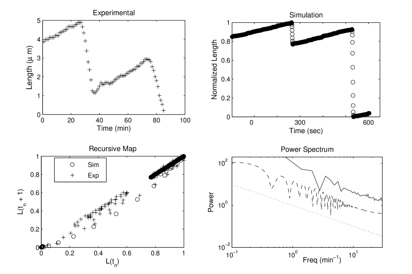
Figure 1:

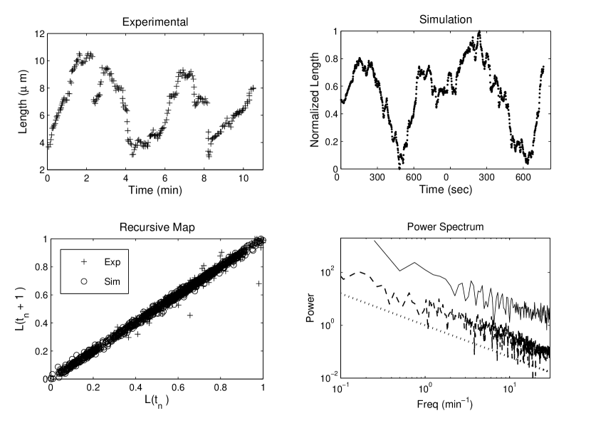
Figure 2:

References

- (1) E. Del Giudice, S. Doglia, M. Milani, G. Vitiello, Nuclear Physics B251 (1985) 375.
- (2) A.S. Davydov, Biology and quantum mechanics (Pergamon, Oxford, 1982).
- (3) A.S. Davydov, Phys. Scripta 20 (1979) 387.
- (4) [3] H. Fröhlich, Rivista del Nuovo Cim. 7 (1977) 399; Advances in Electronics and Electron Physics, ed. L. Marion and C. Matron, vol. 53 (1980) p. 85.
- (5) G. Albrecht-Buehler, Cell and Muscle Motility 6 (1985) 1.
- (6) S. R. Hameroff, Ultimate Computing. Elsevier Science, 1987.
- (7) J. A. Brown, J. A. Tuszynski Phys. Rev. E 56 (1997) 5834.
- (8) A. Priel, J. A. Tuszynski, H. Cantiello, in: E. Bittar and S. Khurana (eds), Ionic Waves Propagation Along the Dendritic Cytoskeleton as a Signaling Mechanism, Molecular Biology of the Cell, Vol. 37, Elsevier, 2006.
- (9) D. K. Fygenson, E. Braun, A. Libchaber, Phys Rev E 50 (1994) 1579.
- (10) D. J. Bicout, Phys Rev E 56 (1997) 6656.
- (11) D. J. Bicout, R. J. Rubin, Phys. Rev. E 59 (1999) 913.
- (12) M. Dogterom, A. C. Maggs, S. Leibler, Proc. Natl. Acad. Sci. USA 92 (1995) 6683.
- (13) M. Dogterom, B. Yurke, Phys. Rev. Lett. 81 (1998) 485.
- (14) M. Dogterom, S. Leibler, Physical aspects of growth and regulation of microtubule structures. Phys. Rev. Lett. 70 (1993) 1347.
- (15) B. Alberts, J. Lewis, M. Raff, K. Roberts, J. D. Watson, Molecular Biology of the Cell, Garland, New York, 1994.
- (16) T. Mitchison, M. Krischner, Nature (London) 312 (1984) 232.
- (17) T. Mitchison, M. Krischner, Nature (London) 312 (1984) 237.
- (18) R. A. Walker, S. A. Inoué, E. D. Salmon, J. Cell. Biol. 108 (1989) 931.
- (19) R. Audenaert, Y. Engelborghs, L. Heremans, K. Heremans Biochim. Biophys. Acta 996 (1989) 110.
- (20) D. J. Odde, L. Cassimeris, H. Buettner, BioPhys. J. 69 (1995) 796.
- (21) H. Flyvbjerg, T. E. Holy, S. Leibler, Phys. Rev. Lett. 73 (1994) 2372.
- (22) H. Flyvbjerg, T. E. Holy, S. Leibler, Phys. Rev. E 54 (1996) 5538.
- (23) T. Antal, P. L. Krapivsky, S. Redner, M. Mailman, B. Chakraborty, Phys. Rev. E 76 (2007) 041907.
- (24) T. Antal, P. L. Krapivsky, S. Redner, J. Stat. Mech. (2007) L05004
- (25) J. M. Dixon, J. A. Tuszynski, J. Appl. Phys. 67 (1990) 5454.
- (26) J. M. Dixon, J. A. Tuszynski, Physica B 163 (1990) 351.
- (27) J. A. Tuszynski, J. M. Dixon, J. Phys. A 22 (1989) 4877.
- (28) J. A. Tuszynski, J. M. Dixon, J. Phys. A 22 (1989) 4895.
- (29) J. A. Tuszynski, J. M. Dixon, Phys. Lett. A 140 (1989) 179.
- (30) J. A. Tuszynski, J. M. Dixon, Physica C 161 (1989) 678.
- (31) J. A. Tuszynski, J. M. Dixon, A. M. Grundland, Fortschritte der Physik (1994) 301.
- (32) J. M. Dixon, J. A. Tuszynski, Phys. Lett. A 155 (1991) 107.
- (33) D. J. Amit, Field Theory, The Renormalisation Group and Critical Phenomena. McGraw-Hill, New York, 1978.
- (34) R. Jackiw, Rev. Mod. Phys. 49 (1977) 681.
- (35) S. K. Ma, Modern Theory of Critical Phenomena. Benjamin, Reading, MA, 1976.
- (36) J. M. Dixon, J. A. Tuszynski, Int. J. Mod. Phys. B 9 (1995) 1611.
- (37) J. A. Tuszynski, D. Sept, J. A. Brown, Physics in Canada, September/October issue (1997) 237.
- (38) M. Caplow, R. L. Ruhlen, J. Shanks, J. Cell Biol. 127 (1994) 779.
- (39) We note that GTP hydrolysis is a subtle biochemical process that carries a quantum of biological energy and thus allows us to make a link between quantum mechanics and polymer dynamics.
- (40) J. A. Tuszynski, J. M. Dixon, Physica A 290 (2001) 69.
- (41) E. Unger, K. J. Bohm, W. Vater, Electron Microsc. Rev. 3 (1990) 355.
- (42) S. Behrens, W. Habicht, J. Wu and E. Unger Surface and Interface Analysis 38, 1014 (2006)
- (43) W. Habicht, S. Behrens, E. Unger, E. Dinjus, Surface and Interface Analysis 38 (2006) 194.
- (44) J. M. Dixon, J. A. Tuszynski, P. L. Clarkson, From Nonlinearity to Coherence; A Study of Universal Features of Many-Body Systems. Oxford University Press, Oxford, 1997.
- (45) E. Mandelkow, E. M. Mandelkow, H. Hotani, B. Hess, S. C. Muller, Science 246 (1989) 1291.
- (46) D. Sept, H-. J. Limbach, H. Bolterauer, J. A. Tuszynski, Journal of Theoretical Biology 197 (1999) 77.
- (47) J. W. H. Sutherland, J. M. Sturtevant, Proc. Natl. Acad. Sci. USA, Vol. 73, No. 10 (1976) 3565.
- (48) I. S. Aranson, L. Kramer, Rev. Mod. Phys. 74 (2002) 99.
- (49) L. Gagnon, P. Winternitz, J. Phys. A: Math. Gen. 21 (1988) 1493.
- (50) L. Gagnon, P. Winternitz, Phys. Lett. A 134 (1989) 276.
- (51) L. Gagnon, P. Winternitz, J. Phys. A: Math. Gen. 22 (1989) 469.
- (52) L. Gagnon, P. Winternitz, J. Phys. A: Math. Gen. 22 (1989) 499.
- (53) L. Gagnon, P. Winternitz, Phys. Rev. A 39 (1989) 296.
- (54) I. S. Aranson, A. R. Bishop, Phys. Rev. Lett. 79 (1997) 4174.
- (55) V. Rezania, O. Azarenko, M. A. Jordan, H. Bolterauer, R. F. Ludue a, J. T. Huzil, J. A. Tuszynski, Biophys. J. ; Published ahead of print on May 23, 2008 as doi:10.1529/biophysj.108.132233
- (56) D. J. Odde, H. Buettner, L. Cassimeris, AIChE J. 42 (1996) 1434.
- (57) H. T. Schek, M. K. Gardner, J. Cheng, D. J. Odde, A. J. Hunt, Microtubule assembly dynamics at the nanoscale. Current Biology 17 (2007) 1445.
- (58) R. Campbell, Information processing in microtubules. PhD thesis, Queensland University of Technology, 2001.
- (59) S. Rasmussen, H. Karampurwala, R. Vaidyanath, K. S. Hensen, S. R. Hameroff, Physica D 42 (1990) 428.
- (60) A. Samsonovich, A. Scott, S. R. Hameroff, Nanobiology 1 (1992) 457.
- (61) J. Tabony, D. Job, Nature 346 (1990) 448.
- (62) S. Portet, J. A. Tuszynski, J. M. Dixon, M. V. Sataric, Stat. Nonlin Soft Matter Phys. 68 (2003) 021903.
- (63) J. A. Tuszynski, M. V. Sataric, S. Portet, J M. Dixon, Phys. Letts. A 340 (2005) 175.
- (64) I. S. Aranson, L. S. Tsimring, Phys. Rev. E 71 (2005) 050901.
- (65) I. S. Aranson, L. S. Tsimring, Phys. Rev. E 74 (2006) 031915.
- (66) R. F. Gildersleeve, A. R. Cross, K. E. Cullen, A. P. Fagen, R. C. Williams Jr., J. Biol. Chem. 267 (1992) 7995.
- (67) E. Shelden, P. Wadsworth, J. Cell Biol. 120 (1993) 935.
- (68) D. Chrtien, S. D. Fuller, E. Karsenti, J. Cell Biol. 129 (1995) 1311.
- (69) D. K. Fygenson, H. Flyvbjerg, K. Sneppen, A. Libchaber, S. Leibler, Phys. Rev. E 51 (1995) 5058.
- (70) I. Arnal, E. Karsenti, A. A. Hyman, J. Cell Biol. 149 (2000) 767.
- (71) S. Pedigo, R. C. Williams Jr., Biophys. J. 83 (2002) 1809.
- (72) N. M. Rusan, C. J. Fagerstrom, A. M. C. Yvon, P. Wadsworth, Mol. Biol. Cell 12 (2006) 971.
- (73) I. A. Vorobjev, T. M. Svitkina, G. G. Borisy, J. Cell Sci. 110 (1997) 2635.
- (74) I. A. Vorobjev, V. I. Rodionov, I. V. Maly, G. G. Borisy, J. Cell Sci. 112 (1999) 2277.
- (75) I. V. Maly, Bulletin Math. Biol. 64 (2002) 213.
- (76) D. J. Odde, Biophys. J. 73 (1997) 88.