The young stellar population of NGC 4214 as observed with HST. II. Results.

Abstract

We present the results of a detailed UV–optical study of the nearby dwarf starburst galaxy NGC 4214 using multifilter HST/WFPC2+STIS photometry. The stellar extinction is found to be quite patchy, with some areas having values of E(4405-5495)$<0.1$ mag and others, associated with star forming regions, much more heavily obscured, a result which is consistent with previous studies of the nebular extinction. We determined the ratio of blue–to–red supergiants and found it to be consistent with theoretical models for the metallicity of the SMC. The stellar IMF of the field in the range $20-100\,\,M_{\odot}$ is found to be steeper than $\gamma=-2.8$ ($\gamma=-2.35$ for a Salpeter IMF). A number of massive clusters and associations with ages between a few and 200 million years are detected and their properties are discussed.

1 Introduction

In this paper we present the results of a comprehensive study of NGC 4214. In Úbeda et al. (2007) (hereafter Paper I) we presented and discussed the deep UV–optical images from two HST instruments: WFPC2 and STIS. We described the methods that we had employed to reduce and analyze our HST images, and we briefly discussed its stellar populations by means of the analysis of two Hertzsprung–Russell [ $\log(T_{\mathrm{eff}})$, $M_{\mathrm{bol}}$ ] diagrams.

In Paper I we made a thorough description of how we used CHORIZOS   (Maíz-Apellániz, 2004), an IDL package that fits an arbitrary family of spectral energy distribution models (SEDs), to analyze our multi–color photometric data. We applied CHORIZOS to stars and clusters separately, using different input SEDs. In this present work we show and discuss the results.

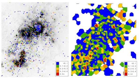
Figure 1: [Left panel] F656N mosaic of NGC 4214 where we have over–plotted the selection of stars that we used to make the extinction map. The color scale represents values of $E(4405-5495)$ [Right panel] Extinction map of the central region of NGC 4214. The orientation is north pointing up and east pointing to the left. The field dimensions are 875 pc $\times$ 972 pc or $61\farcs 4\times 68\farcs 3$. The cluster apertures are also drawn for reference. See the text for a description of how we made this map.

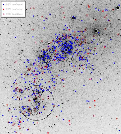
Figure 2: Distribution of blue and red supergiants on an F814W mosaic of NGC 4214. The field shown is the same as in Figure 1. The filled circles represent the confirmed supergiants, both blue and red that we used to calculate the B/R ratio. With open red circles we represent the group of stars that follow the criteria $\log(T_{\mathrm{eff}})\leqslant 3.70$ and $M_{\mathrm{bol}}\leqslant-6.0$. and which might be RSGs, AGBs/ bright RSGs. The cluster apertures are also drawn for reference.

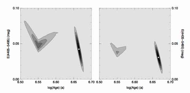
Figure 4: Reddening vs. age likelihood contour plots for cluster I–As provided as output by CHORIZOS and obtained using Starburst99 models. [Left] Contour plot obtained using the LMC2 extinction law. [Right] Contour plot obtained using the SMC extinction law. Note that the age of this cluster is in the range 3.0–4.5 Myr, and that it is characterized by a very small extinction. The white circle marks the most likely value (mode).

NGC 4214 (see Figures 1, 2 and 4 in Paper I) is a nearby ($2.94\pm 0.18$ Mpc; Maíz-Apellániz et al. (2002)) dwarf galaxy (de Vaucouleurs et al., 1991) with a low metallicity content $(Z=0.006)$ (Úbeda et al., 2007). It has two main regions of star formation which we studied using high–resolution images obtained from three HST archival proposals: 6716 (P.I.: Theodore Stecher), 6569 (P.I.: John MacKenty), and 9096 (P.I.: Jesús Maíz-Apellániz).

NGC 4214 possesses a combination of properties (high star formation rate, proximity, low extinction, spatially well resolved) that make it a perfect candidate for astrophysical studies of young stellar populations, which we investigate in the present work. We analyze the ratio of blue to red (B/R) supergiants, the initial stellar mass function (IMF), and the properties of its young– and intermediate–age cluster population. We also study the variable extinction across the galaxy.

In order to advance the understanding of massive stars it is important to have an observational database with which the predictions of stellar evolutionary theory may be compared and refined. In particular, the ratio B/R of the blue to red supergiants is a major characteristic of the luminous star population in galaxies. van den Bergh (1968) first suggested the B/R ratio varied among nearby galaxies as a result of the effect of metallicity on massive star evolution. Several studies confirmed that the B/R ratio is an increasing function of metallicity (Langer & Maeder, 1995; Eggenberger et al., 2002). This fact is known as a result of studies in the Galaxy (Humphreys & McElroy, 1984) and the Magellanic Clouds (Humphreys, 1983; Massey & Olsen, 2003). This ratio has also been studied in M33 (Walker, 1964; Humphreys & Sandage, 1980) and more recently in Sextans A by Dohm-Palmer & Skillman (2002). In this paper we examine the B/R ratio for NGC 4214.

Kroupa (2002) presents an updated review of our current knowledge of the IMF for different types of stars. This function is particularly important for the most massive stars (Garmany et al., 1982) which evolve very quickly and strongly influence their environment via stellar winds and mass loss. Massey et al. (1995a, b) studied the massive star content of OB associations in the Milky Way and the Magellanic Clouds and found that there is no difference in the IMF slope between the MW, the LMC and the SMC; therefore, to first order, metallicity does not appear to affect the IMF of massive stars, at least over the factor of 5 spanned between the SMC ($Z=0.004$), the LMC ($Z=0.008$) and the MW ($Z=0.02$). OB associations have been discovered in some Local Group galaxies, and with the fine spatial resolution provided by the HST, it is possible to obtain the stellar IMF of those systems. Recent works include M31 (Veltchev et al., 2004), M33 (González Delgado & Pérez, 2000), IC10 (Hunter, 2001), and IC1613 (Georgiev et al., 1999). The previous work on the IMF of NGC 4214 has been based on the integrated spectrum of the galaxy (Leitherer et al., 1996; Chandar et al., 2005). Here we present the first work on its IMF based on high–resolution HST imaging.

Stellar clusters have long been recognized as important laboratories for astrophysical research. They are extremely useful in different aspects of Astronomy: they provide classical tests of stellar evolution, they can be used for studies of stellar dynamics and they provide an understanding of the galactic structure (Lada & Lada, 2003). Young clusters are tracers of recent star formation; they form in giant molecular clouds (GMCs) and they remain embedded or close to their parent cloud during the first $\approx 1$ Myr, making it difficult to study them in their early stages. However, recent developments in infrared imaging cameras have led to the conclusion that young embedded clusters are numerous, and that a significant fraction of all stars may form in such systems. Massive Young Clusters (MYCs) can be divided into Super Star Clusters (SSCs), which are organized around a compact core (size $\approx 1-3$ pc), and Scaled OB Associations (SOBAs) which lack such a structure and are more extended objects (size $>10$ pc). SSCs are bound objects and represent the high–mass end of young stellar clusters while SOBAs are unbound and are the massive relatives of regular OB associations (Maíz-Apellániz, 2001). MYCs have been discovered in various environments, including our Galactic Center, in the nuclei of late–type galaxies, in nearby starburst galaxies and in merging galaxies.

The present paper is organized as follows: In Section 2 we present the study of the extinction throughout NGC 4214; in Section 3 we analyze the B/R ratio; the IMF is addressed in Section 4; in Section 5 we perform a detailed study of some interesting clusters. Finally, in Section 6 we summarize our results and provide the conclusions.

2 Extinction

A comparison between stellar atmosphere models and observed colors can be used to infer the extinction toward individual stars. For our study, we used the IDL code CHORIZOS (Maíz-Apellániz, 2004); this program (see Section 2.5 in Paper I) reads unreddened SED models, extinguishes them and obtains the synthetic photometry that is compatible with the input colors. In this way we obtained the extinction law that best agrees with the data, and the extinction value [ $E(4405-5495)$ ]  for each star in our main photometric lists: LIST336 (built with F336W as reference filter) and LIST814 (built with F814W as reference filter) as described in Paper I. For the extinction law, we considered the $R_{5495}-$dependent family of Cardelli et al. (1989) (Galactic extinction); the average LMC and LMC2 laws of Misselt et al. (1999) (extinction of the LMC), and the SMC law of Gordon & Clayton (1998) (extinction of the SMC). CHORIZOS also provides the uncertainties $\sigma$ of the calculated parameters.

In previous studies of NGC 4214, the extinction correction was performed using different values of $E(B-V)$: Maíz-Apellániz et al. (1998) measured a variable $E(B-V)$ with values between 0.0 and 0.6 mag from the ratio of the nebular emission lines H$\alpha$ to H$\beta$. Maíz-Apellániz et al. (2002) measured an average value of $E(B-V)=0.09$ mag from the optical colors of the young stellar population far from the main star–forming complexes. Drozdovsky et al. (2002) and Calzetti et al. (2004) adopted the value $E(B-V)=0.02$ mag provided by the IRAS DIRBE map of Schlegel et al. (1998). All those estimates assume a Cardelli et al. (1989) extinction law with $R_{5495}=3.1$.

In order to develop an extinction map of NGC 4214, we made a selection of objects from LIST336, using the following criteria: We considered all the objects with $\sigma_{E(4405-5495)}\leqslant 0.1$ mag for those stars with $E(4405-5495)\leqslant 0.4$ mag. This selection yields 855 objects with $<{\mathrm{F}336W}>=20.93$ and $<\sigma_{\mathrm{F}336W}>=1.22$. Objects with $E(4405-5495)>0.4$ mag were selected on the basis of their F336W magnitude (F336W $<21$ mag) and their location within the galaxy. We made no restriction according to photometric or extinction error in this case. We found 43 objects with $E(4405-5495)>0.4$ and they present $<E(4405-5495)>=0.54$ mag and $<\sigma_{E(4405-5495)}>=0.21$ mag. Using this biased sample of objects, we may be underestimating the extinction values and probably missing some blue objects. It is important to note that extinction is a complicated three-dimensional effect which involves stars, nebulae and dust and which varies at small ($\lesssim 1$ pc) scales. All these facts contribute to make extinction–modelling quite difficult. Finally, we added the results of the extinction analysis (Section 5.1) for clusters I–As, I–Es, IIIs, and IVs to our list. The left panel of Figure 1 is an F656N mosaic of the surveyed region of NGC 4214, where we have marked the objects in our final list with a color scheme to indicate the extinction distribution throughout the galaxy. To build the H$\alpha$ (filter F656N) mosaic, we used images u3n8010fm + gm from proposal 6569. The total exposure time is 1600 sec. This mosaic clearly shows the patchy nature of the extinction.

To build the extinction map, we created a spatial grid $M$ and assigned a weighted value of the extinction to each pixel in the grid. The procedure follows: We first calculated the distance $d_{ijk}$ (in WF pixels of $0\farcs 1$) between each pixel in the grid $M[i,j]$ and all the stars $k$ in our list. We then calculated a weight with

$$w_{k}=\frac{\exp\left(-\frac{d_{ijk}^{2}}{30}\right)}{\sigma_{E_{k}}^{2}},$$ (1)

where $\sigma_{E_{k}}$ is the error in $E=E(4405-5495)$ for star $k$, and the value 30 is a scale factor. We used several values of the scale factor to represent the extinction map, and we present here the map with the one that best showed the different extinction regions. The value associated to the pixel $M[i,j]$ is given by

$$M[i,j]=\frac{\sum_{k}E_{k}\cdot w_{k}}{\sum_{k}w_{k}}$$ (2)

The extinction map is shown in the right panel of Figure 1. The most prominent feature in this map is the fact that NGC 4214 is characterized by low values of the extinction, except for some well defined regions with high values, which is in agreement with Maíz-Apellániz et al. (1998), Drozdovsky et al. (2002), and Calzetti et al. (2004). In Section 5 we discuss in more detail the regions around some of the clusters.

Maíz-Apellániz et al. (1998) and Maíz-Apellániz (2000) used the Balmer ratio (H$\alpha$/H$\beta$) as a tracer of the reddening that affects the ionized gas and produced maps of this ratio. Their analysis showed a significant difference between the two most prominent complexes in the galaxy: NGC 4214–I and NGC 4214–II. Their conclusions are that the nebular emission and stellar continuum are produced in co–spatial or close regions in NGC 4214–II, while the emitting gas is clearly spatially offset with respect to the stellar cluster in the brightest knots on the NGC 4214–I complex. They also find that the reddening in NGC 4214–II is, on average, higher than in NGC 4214–I. Our results, derived from the stellar colors, validate those points. The two main cavities in NGC 4214–I show low extinction surrounded by higher values while for NGC 4214–II the extinction is higher overall.

Walter et al. (2001) present an interferometric study of the molecular gas in NGC 4214. They detect three regions of molecular emission, in the northwest, southeast, and center of the galaxy. These authors compared the structure of the molecular tracer, CO, with tracers of star formation like H$\alpha$. Two of the three CO complexes are associated directly with star–forming regions. The southeastern CO clump appears co–spatial with NGC 4214–II. The peak of the CO emission is almost on top of one of the clusters. Our extinction map shows a high extinction region co–spatial with this molecular cloud. The central CO emission is associated with the largest region in H$\alpha$ emission, spanning most of the NGC 4214–I region. This CO complex is diffuse instead of centrally concentrated, and the peak of the CO emission is shifted to the west of the peak of the H$\alpha$ emission, with little CO seen at the location of the two main cavities. Overall, our extinction map traces the molecular cloud in this part of the galaxy too, although with less detail.

The extinction derived from the stellar continuum is similar to the extinction derived via the analysis of nebular lines across the galaxy, and this is true on a star by star basis. The coincidence is fairly good throughout the galaxy.

3 The ratio of blue–to–red supergiants

The ratio B/R of the blue to red supergiants of initial masses larger than 15 $M_{\sun}$ is an important observable of the luminous star population in galaxies and it is one of the stellar properties that can be easily measured beyond the Local Group. This quantity depends strongly on the model parameters and it can be used to constrain the model physics very accurately. This ratio has been calculated in Galactic clusters and in some clusters in the LMC and SMC. Both Eggenberger et al. (2002) and Langer & Maeder (1995) present comprehensive reviews of past studies.

The main result from previous observational studies is that, for a given luminosity range, B/R steeply increases with increasing metallicity $Z$, by a factor of about 10 between the SMC and the inner Galactic regions. Current theoretical models of massive stars are unable to correctly reproduce the changes of B/R with metallicity, from solar to SMC value. It is known that the B/R ratio is a sensitive quantity to mass loss, rotation, convection and mixing processes, hence it constitutes an important and sensitive test for stellar evolution models if it were fully understood.

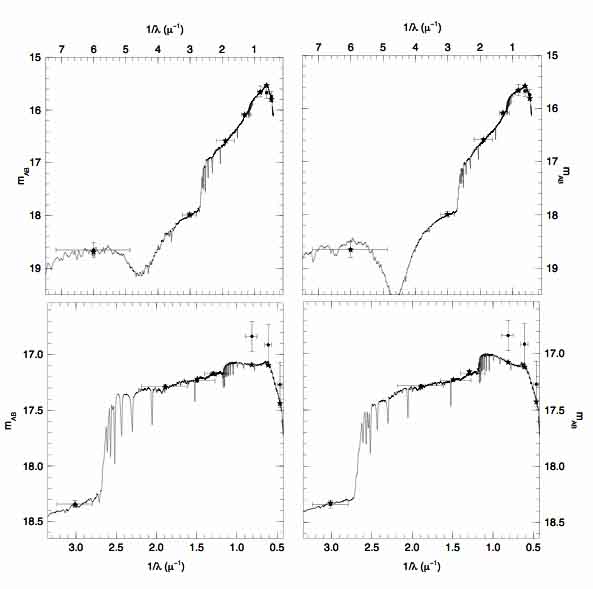
Figure 8: Same as Figure 3 for clusters IIIs and IVs. [Top left] Best fit SED for cluster IIIs for the old (167 Myr) solution. [Top right] Best fit SED for cluster IIIs for the young (16 Myr) solution. [Bottom left] Best fit SED for cluster IVs for the old (150 Myr) solution. [Bottom right] Best fit SED for cluster IVs for the young (16 Myr) solution.

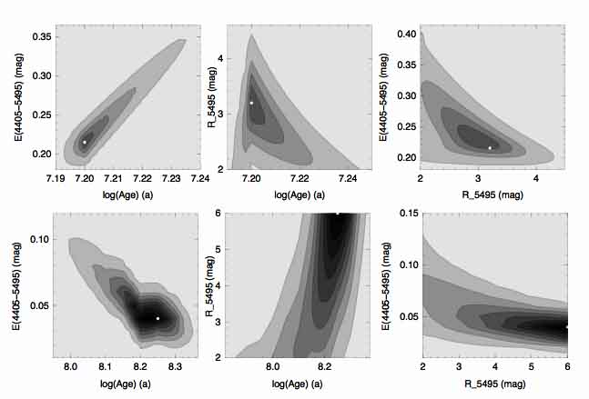
Figure 9: Likelihood contour plots for cluster IVs provided as output by CHORIZOS and obtained using Starburst99 models. The upper row corresponds to the young solution and the lower row to the old one. [Left] Reddening vs. age plot. [Center] Extinction law vs. age. [Right] Extinction law vs. reddening. Age is expressed in years. The white circle marks the most likely value (mode).

In this paper we present our results for NGC 4214. The B/R value is dependent on how stars are counted, and thus disagreement with the predictions of stellar evolutionary models have to be carefully evaluated. Notice that the definition of B/R is not always the same. We followed the method suggested by Maeder & Meynet (2001). We count in the B/R ratio the B star models from the end of the main sequence to type B9.5 I, which corresponds to $\log(T_{\mathrm{eff}})=3.99$ according to the calibration by Flower (1996). We count as red supergiants all star models below $\log(T_{\mathrm{eff}})=3.70$. In both cases we considered stars located between the 15 and 25 $M_{\sun}$ evolutionary tracks. Figures 8 and 9 in Paper I show the detailed evolutionary tracks of non–rotating stellar models for initial masses between 5, 7, 10, 12, 15, 20, 25, 40, and 120 $M_{\sun}$, LMC–like metallicity $(Z=0.008)$ from Schaerer et al. (1993). Two vertical lines (at $\log(T_{\mathrm{eff}})=3.99$ and $\log(T_{\mathrm{eff}})=3.70$) mark the limits between the blue supergiants locus and the position of the red supergiants. The location of the blue and red supergiants is marked in those Figures with two polygons between the 15 and 25 $M_{\sun}$ tracks. We used Figure 8 in Paper I to count red supergiants and Figure 9 in Paper I to count blue supergiants.

Several studies identify supergiants by considering objects brighter than $M_{\mathrm{bol}}=-7.5$ mag which corresponds to masses larger than 15 $M_{\sun}$ for red supergiants. If a lower luminosity is chosen there is a chance of contamination by intermediate asymptotic giant branch (AGB) stars (Brunish et al., 1986). We avoided this problem by selecting objects located above the 15 $M_{\sun}$ evolutionary track in all cases. We performed an analysis to study how the stars located below the 15 $M_{\sun}$ evolutionary track would contaminate those which we consider red supergiants. For this contamination analysis we generated artificial stars with masses that place them below the 15 $M_{\sun}$ evolutionary track and used the typical uncertainties obtained from CHORIZOS for $T_{\mathrm{eff}}$ and $M_{\mathrm{bol}}$ to modify their positions in the H–R diagram accordingly. Then, using the observed distribution below the 15 $M_{\sun}$ track, we tested whether a significant number could have “leaked” to a higher mass bin due to the experimental uncertainties. The contamination thus calculated was found to be less than 1%, so a correction was not applied. For our analysis, we assumed that we are considering single stars and therefore no correction for blends of single stars was performed.

In order to compare our observational results with what theory predicts, we calculated the B/R ratio values using three grids of theoretical models from the Geneva database: [1] the evolutionary tracks of non–rotating ($v_{ini}=0$ km s^-1) stellar models for initial masses between 9 and 60 $M_{\sun}$ and SMC–like metallicity $(Z=0.004)$ (Maeder & Meynet, 2001); [2] the evolutionary tracks of rotating ($v_{ini}=300$ km s^-1) stellar models for initial masses between 9 and 60 $M_{\sun}$ and SMC–like metallicity $(Z=0.004)$ (Maeder & Meynet, 2001); and [3] the evolutionary tracks of non–rotating stellar models for initial masses between 10 and 120 $M_{\sun}$, LMC–like metallicity $(Z=0.008)$ (Schaerer et al., 1993). We did not find any major difference between models with high and normal mass–loss rates, so we adopted normal mass–loss rates evolutionary tracks. Unfortunately, evolutionary tracks of rotating ($v_{ini}=300$ km s^-1) stellar models with LMC–like metallicity are not available in the literature.

The ratio of the densities of blue supergiants to red supergiants at a given initial mass is equal to the ratio of the lifetimes along the evolutionary tracks in the corresponding $\log(T_{\mathrm{eff}})$ intervals. The resulting theoretical B/R values are given in Table 1.

In order to count the number of blue and red supergiants in our lists, we had to apply corrections based on our completeness tests. We used the completeness values described in Section 2.3 of Paper I, which we summarized in its Table 3. We calculated the completeness values for two intervals of $\log(T_{\mathrm{eff}})$ along each evolutionary track: from the end of the main-sequence to $\log(T_{\mathrm{eff}})=3.99$ and for the interval $\log(T_{\mathrm{eff}})\leq 3.70$. For each of the points that define the evolutionary tracks we interpolated linearly in the completeness tables to calculate their completeness value. We also computed a weight defined as the difference between the age of this point on the evolutionary track, and the age of the same point in the immediately older evolutionary track. The adopted completeness value is the weighted mean in each interval.

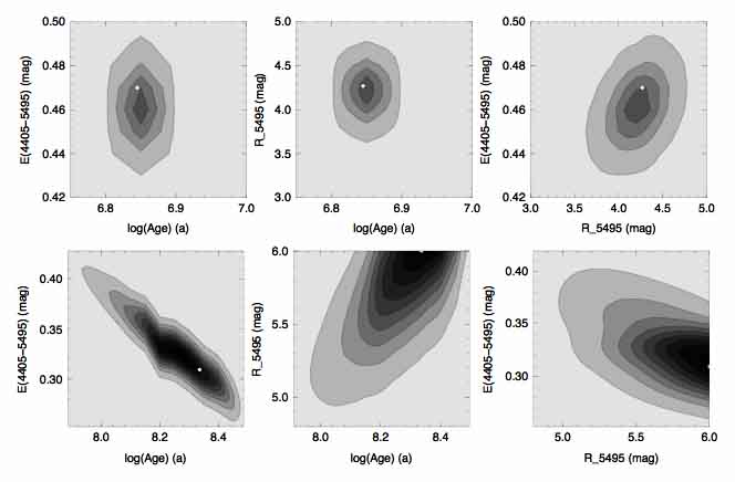
Figure 5: Likelihood contour plots for cluster I–Es provided as output by CHORIZOS and obtained using Starburst99 models. The upper row corresponds to the young solution and the lower row to the old one. [Left] Reddening vs. age plot. [Center] Extinction law vs. age. [Right] Extinction law vs. reddening. Age is expressed in years. The white circle marks the most likely value (mode). Note that the mode in 3D parameter space (shown here) does not necessarily coincide with the mode in 2D parameter space.

Counting the blue supergiants in our sample presented no problem; we simply calculated the number of stars within each mass range provided by the evolutionary tracks. However, if we compare the distribution of red supergiants in the Hertzsprung–Russell diagram to that of the various stellar evolutionary models, we find that none of the models produce RSGs as cool and luminous as what is actually observed. This fact was noted by Massey (2003), and Massey & Olsen (2003). They found the same problem while trying to account for the RSG content in the Magellanic Clouds. In their work, the sample of RSGs includes both stars with known spectral type and a group of objects with known photometry but no spectroscopy. They plot those supergiants in [$\log(T_{\mathrm{eff}})$, $M_{\mathrm{bol}}$] planes and overplot several sets of evolutionary tracks. They use a new calibration between spectral type and $\log(T_{\mathrm{eff}})$ to place stars with known spectral type. For the rest of the stars, they use the intrinsic color $(V-R)_{0}$. Whatever the method to place the stars in the diagram, we can argue that there is no significant difference. Their Figure 5(a) for the LMC RSGs is quite similar to our Figure 8 in Paper I. It is important to note that our method is strictly photometric, because CHORIZOS fits the best known SEDs from Kurucz (2004) to a set of observed photometric colors.

In order to count the RSGs in our sample we had to artificially extend the evolutionary tracks at constant values of $M_{\mathrm{bol}}$, and used the region marked by a small rectangle located between the 15 and 25 $M_{\sun}$ tracks in Figures 8 and 9 in Paper I to the right of $\log(T_{\mathrm{eff}})=3.70$. After counting the red and blue supergiants in our lists we corrected these numbers for incompleteness. A summary of the results of the ratio B/R is presented in Table 1. There, the columns labeled “theory” show the numbers derived from the ratio of time spent by a star in each region and, therefore, assumes a constant star formation rate. The “observation” columns show the numbers previously described in this paragraph.

Figure 2 shows the distribution of blue and red supergiants on an F814W mosaic of NGC 4214. The filled circles represent the confirmed supergiants, both blue and red that we used to calculate the B/R ratio. With open red circles we represent the group of stars that follow the criteria $\log(T_{\mathrm{eff}})\leqslant 3.70$ and $M_{\mathrm{bol}}\leqslant-6.0$. The latter objects may be either RSGs, AGB stars, or even bright red giants that have “leaked” into higher–mass regions in the H–R diagram due to observational uncertainties.

Despite the difficulty in counting RSG because the computed grids do not produce RSGs as cool and luminous as what we observe, we find a good agreement between our data and the non–rotating models with low metallicity $(Z=0.004).$ These models predict a B/R value of 24 in the $15-20\,M_{\sun}$ mass–range, and we measure $34\pm 10$. Some of the stars below the 15 $M_{\sun}$ track may be RSGs, so we are underestimating the real number of RSGs. In the mass–range $20-25\,M_{\sun}$ the theoretical prediction is 47 and we obtain $46\pm 23$. In both cases, our results agree with the theoretical ones within Poisson errors.

There are two caveats regarding this result that should be mentioned. First, the small quantity of confirmed RSGs in our sample in NGC 4214 imply that stochastic effects due to small–number statistics may be present. However, given the large differences in the theoretical ratios shown in Table 1, this effect is likely to be unimportant. The second caveat is related to the conversion from observed colors to effective temperatures and bolometric magnitudes. Levesque et al. (2005) present a new effective temperature scale for Galactic RSGs by fitting MARCS stellar atmosphere models (Gustafsson et al., 1975; Plez et al., 1992) which include an improved treatment of molecular opacity to 74 Galactic $(Z=0.020)$ RSGs of known distance. They compare their location on the [$\log(T_{\mathrm{eff}})$, $M_{\mathrm{bol}}$] plane with theoretical evolutionary models from Meynet & Maeder (2003) and find a much better agreement between theory and observation. Their main result is that RSGs appear to be warmer than previously thought. This effect shifts the stars to the left in the diagrams making them coincide with the end of the tracks. It would be interesting to compare the change of temperature from the fitting of observed optical colors using CHORIZOS or a similar code from Kurucz to MARCS atmospheres to verify if it accounts for the $350-400$ K discrepancy detected in our data. More importantly, such a change should also shift the stars downwards in the H–R diagram, since a higher temperature implies a lower bolometric correction.

At the time in which we performed our fits, CHORIZOS did not have the capability to fit stellar models other than Kurucz or Lejeune. It is in our future plans to reanalyze this data using the MARCS stellar atmospheres models.

4 Initial mass function

4.1 The IMF of the resolved population

A lot of effort has been put into obtaining the IMF of the Milky Way and the Magellanic Clouds in the past decades. Star counts in clusters/associations in those local galaxies reveal an IMF with a slope close to Salpeter $(\gamma=-2.35)$ above $\sim 1M_{\odot}$ (Schaerer, 2003) when a power law of the form $\frac{dN}{dm}=A\,m^{\gamma}$ is used. Massey (1998) concludes that there is no difference in IMF slopes found between the Milky Way, the LMC and SMC. He claims that the weighted average of the IMF slopes of the MW is $\gamma=-2.1\pm 0.1$; and that of the MCs is $\gamma=-2.3\pm 0.1$. This shows that metallicity does not affect the IMF slopes of massive stars.

It has long been known that some very massive stars are not currently found in clusters or associations, but they seem to be part of the field (Massey, 1998). Studies of the MCs showed that very massive stars can be found in highly isolated regions, and that they are the result of small star–forming events. An IMF study of these field objects led to surprising results: the actual IMF slope is quite steep, with $\gamma\sim-5$ (Massey et al., 1995b). This trend is found in the MCs and the Milky Way as well, and is easily detected in the spectral type distribution (van den Bergh, 2004). It is currently debated whether the difference in slopes is due to differences between in situ formation styles or to a majority of field O stars being runaways (de Wit et al., 2004).

What do we know about the stellar IMF above $\sim 1M_{\odot}$ for galaxies beyond the MCs? There are several problems involved in the determination of IMFs in extragalactic systems. Only a few galaxies are close enough for star counts to be carried out with any reliability, and even these are so distant that only the very brightest part of the luminosity function can usually be sampled. In addition, there are practical problems with star counts in external galaxies, including crowding, incompleteness, and corrections for foreground stars. Among other studies, Veltchev et al. (2004) studied the IMF of M 31 and derived a slope of $\gamma=-2.59\pm 0.09$; Jamet et al. (2004) found an IMF slope of $\gamma=-2.37\pm 0.16$ for the ionizing cluster of NGC 588 in the outskirts of the nearby galaxy M 33; Annibali et al. (2003) analyzed the star formation history of NGC 1705 and inferred an IMF slope close to Salpeter.

The most direct and reliable method of obtaining the IMF of a certain stellar population is based on counts of stars as a function of their luminosity/mass. However, there are other indirect methods which do not employ star counts, but still yield some information on the IMF (Scalo, 1986). One of these is the method of population synthesis, which attempts to match the observed galaxy colors, spectrum or line strengths by finding the best mixture of stars of various spectral types and luminosity classes. The main problems that arise with this method are the uniqueness of the solution and the types of astrophysical constrains that need to be imposed on the data.

Chandar et al. (2005) apply this method to estimate the IMF slope in the field stars of NGC 4214. They assume that the faint intra–cluster light in NGC 4214 corresponds to the field stars in the galaxy. They compared the spectroscopic signature with Starburst99 evolutionary synthesis models and found a lack of strong O–star wind features in the spectra, which led them to conclude that the field light originates primarily from a different stellar population, and not from scattering of UV photons leaking out of the massive clusters. Fitting IMF slopes in continuous–formation Starburst99 models they infer that the best value for NGC 4214 would be $\gamma=-3.5$. Their work also provides similar values of the IMF slope for other local starburst galaxies such as NGC 1741, NGC 3310, and NGC 5996.

Comparing low resolution spectra taken with the International Ultraviolet Explorer (IUE) in the 1100–3200 Å range with the predictions of evolutionary population synthesis models, Mas-Hesse & Kunth (1999) obtain $\gamma=-3.0$ for the sum of field and clusters in NGC 4214.

4.2 Method and sample selection

Determining the IMF of a stellar population with mixed ages is a difficult problem. Stellar masses cannot be weighed directly in most instances, so the mass has to be deduced indirectly by measuring the star’s luminosity and evolutionary state. We followed the photometric/spectroscopic method provided by Lequeux (1979): we estimated bolometric magnitudes ($M_{\mathrm{bol}}$), and effective temperatures ($T_{\mathrm{eff}}$) for each star in the sample, as we explain in Paper I. The present–day mass function was estimated by counting the number of stars in the Hertzsprung–Russell diagram between theoretical evolutionary tracks computed for models with different masses. In the case of a coeval star–formation region, the obtained function is the IMF modified by evolution at the high–mass end. For a continuous star formation region, the IMF followed by division of the number of objects in each mass range by the main sequence lifetime $(\tau_{MS})$ of the corresponding mass.

For the IMF determination, we used the theoretical evolutionary tracks from Lejeune & Schaerer (2001) in the mass range 5 to 120 $M_{\odot}$. These theoretical models provide 51 values of $T_{\mathrm{eff}}$, $L$ and age for each evolutionary track for a given metallicity. The first 11 points of each track define their main–sequence sections. A line connecting the first point of each track defines the zero age main–sequence (ZAMS). This line is the left boundary of our main–sequence. A line connecting the 11th point of each track defines the right boundary of the main–sequence.

Here we present a detailed analysis of the IMF of NGC 4214 using two key assumptions: (i) we selected only main–sequence stars from our sample, and (ii) we assumed that the IMF has remained constant as a function of time. Figure 2 in our Paper I shows three regions of strong H$\alpha$  emission, which can be matched to active recent star–forming regions. These regions are I–A, I–B and II. In LIST336 we found a total of 3061 objects located along the main–sequence band. We considered three lists of masses to calculate the IMF: (1) LIST1: a list including all objects (3061 stars), (2) LIST2: a list with objects in regions I–A, I–B and II (active star–forming regions) (900 stars), and (3) LIST3: a list with all objects except those of I–A, I–B and II (2161 stars.) We assumed all binary and higher–order stellar systems are resolved into individual stars. See Section 4.3.3 for a detailed discussion on multiplicity.

We started by determining the stellar masses and their errors of all objects in the lists using the estimated values of $M_{\mathrm{bol}}$ and $T_{\mathrm{eff}}$ obtained with CHORIZOS as described in Paper I. We plotted a Hertzsprung–Russell diagram [$\log$ $T_{\mathrm{eff}}$, $M_{\mathrm{bol}}$] on which we superimposed theoretical evolutionary tracks from Lejeune & Schaerer (2001) in the mass range $5-120M_{\odot}$. We then isolated the main–sequence sections of those tracks and we obtained interpolated mass values between the tracks using splines. We built an IDL code that triangulates the whole grid and interpolates the data to obtain a finely spaced grid of masses throughout the whole Hertzsprung–Russell diagram. This procedure gave us a two variable function $M=f($ $T_{\mathrm{eff}}$, $M_{\mathrm{bol}}$ ) which assigns a mass $(M)$ value from the input values $M_{\mathrm{bol}}$ and $T_{\mathrm{eff}}$. The individual stellar masses $(M_{i})$ followed directly from this function. To obtain the uncertainties $(\sigma_{M_{i}})$ for the individual masses $(M_{i})$, we created a randomly distributed set of 10000 points around the mean values of $T_{\mathrm{eff}}$  and $M_{\mathrm{bol}}$  for each star and inferred their individual masses. Those points were distributed using a bidimensional gaussian distribution according to the parameters provided by the output of CHORIZOS. The standard deviation of these masses gave us a reliable value of the error $(\sigma_{M_{i}})$ in the mass $(M_{i})$ of each star. How dependent are our results on the evolutionary models used for the mass tracks in the Hertzsprung–Russell diagram ? We found that the locus of an evolutionary track of a given mass on the Hertzsprung–Russell diagram, changes with initial conditions such as metallicity, mass–loss, rotation, etc. Most of them show loops which give them a complex shape. However, these changes are minor and may be neglected when we consider the uncertainty in the mass determination for the objects in our lists, especially since we are considering objects that lie within the limits of the main sequence where those changes are insignificant. The covariance ellipse for each single object, usually spans a wide range of evolutionary tracks (due to the intrinsic errors in the determination of $T_{\mathrm{eff}}$ and $M_{\mathrm{bol}}$ from CHORIZOS.) This would have not changed if we had chosen a different set of theoretical models. It is important to note that the most massive objects in our lists have smaller relative errors than the less massive ones. How does that translate into the determination of the error in the mass of each star? Even though the most massive objects have smaller errors in $T_{\mathrm{eff}}$ and $M_{\mathrm{bol}}$, their errors in mass may still be large because their covariance ellipses extend over a wider range of masses. On the other hand, objects with lower masses have bigger errors in $T_{\mathrm{eff}}$ and $M_{\mathrm{bol}}$, but their location in the Hertzsprung–Russell diagram is such that their ellipses span a narrower range of evolutionary tracks.

Regions I–A, I–B and II are young clusters with recent bursts of star formation. They all have different ages as we will show in Section 5. For these regions, we considered that the present–day mass function is the IMF. The rest of the galaxy is composed of a large number of star–forming regions of different ages, and a fairly good approximation would be to consider it as a region of continuous star formation. For this case we corrected the star counts for the main–sequence life–time $\tau_{MS}$ at each particular mass, using values from Table 4 in Paper I.

4.3 Correction of systematic effects

In order to determine the IMF of our sample of stars, we analyzed four sources of systematic effects, as pointed out by Maíz-Apellániz et al. (2005): (1) data incompleteness, (2) appropriate bin selection, (3) unresolved objects in our sample, and (4) mass diffusion.

4.3.1 Data incompleteness

In the derivation of an IMF, a quantitative evaluation of completeness of the photometric data is required. To obtain the completeness values along the main–sequence section of each evolutionary track, we calculated its value on each point that defines the main–sequence using the results from Section 2.3 in Paper I; we also computed a weight defined as the difference between the age of this point on the evolutionary track, and the age of the corresponding point in the nearest more massive evolutionary track. The adopted completeness value is the weighted mean in each interval. All values are summarized in Table 4 in Paper I. We determined the main–sequence lifetime of each available track by interpolating among the ages provided by the models.

4.3.2 Bin selection

To calculate the slope of the IMF we followed the technique suggested by Maíz Apellániz & Úbeda (2005) and used a weighted least square method to fit a power law $\frac{dN}{dm}=A\cdot m^{\gamma}$ using 5 bins of variable size, so that the number of stars in each bin is approximately constant. This method guarantees that the binning biases will be minimum and that the uncertainty estimates are correct. For each bin, we used the weight $w_{i}$ derived from a binomial distribution as suggested by Maíz Apellániz & Úbeda (2005).

4.3.3 Unresolved objects

In distant stellar systems like the MCs or NGC 4214, we encounter a serious problem: namely, crowding of stellar images which makes the IMF determination somewhat complicated. At the distance of NGC 4214 (2.94 Mpc), 1 arcsec corresponds to $\approx$14 pc. We therefore expect some of the regions in the galaxy to be crowded from the observational point of view. We may find unresolved objects in our sample, i.e., merged stellar images, irrespective of their nature as a physical system or a chance coincidence. The reliability of the highest mass stars is questionable because of stochastic effects due to small number statistics and evolutionary effects. Some stellar evolution has certainly taken place for these stars and some of them may fall out of the main–sequence band.

The effect of unresolved objects in a sample used to determine a stellar IMF has been already analyzed by several authors. Sagar & Richtler (1991) studied the effect of actual binaries in the mass range $2-14~{}M_{\odot}$ by performing several Monte-Carlo experiments using initial values $\gamma=-3.5,-2.5,$ and $-1.5$ and several binary fractions. They come to the conclusion that the general effect is a flattening of the mass function. With an intrinsic slope of $\gamma=-3.5$ there is hardly any influence on the MF slope; and for $\gamma=-2.5$ the MF slope undergoes a flattening of 0.34 if the binary fraction increases to 50%. They made the assumption that stellar masses are distributed randomly among the components. Kroupa et al. (1991) show that unresolved binary stars have a significant effect on any photometrically determined luminosity function. Their research leads to the conclusion that when binaries are not taken into account, there is an underestimate on the number of low mass stars, leading to a flattening of the IMF slope. Given the large multiplicity fractions observed for OB stars, this effect must be significant for intermediate– and high–mass stars (Maíz-Apellániz et al., 2005). However, since the binary fraction is unknown in our sample, it is not possible to correct the estimated values of the IMF slope for the presence of binaries. We used $M_{up}=100M_{\odot}$ as the high–mass end of the integration which allowed us to discard some unresolved objects in our sample, but this effect is difficult to solve for a galaxy located at the distance of NGC 4214 because, even with the high–resolution images provided by HST, we still observe multiple systems.

One additional source of multiple objects is the blends of stars caused by chance alignments. The greater the distance to the object of study, the more likely one is prone to encounter these kind of objects. Our analysis of multiple systems leads us to conclude that the real value of the slope would be steeper than the value that we obtain with our study.

For the low–mass end of the integration, we used several mass values in the range $6,6.5,...,25M_{\odot}$. The main problem regarding the low–mass end is the completeness of our data, because the observational sensitivity limit is reached here. We corrected the number of counts for incompleteness using the values given in Table 4 in Paper I, as described above. The IMF slope values that we present were calculated for $M_{low}=20M_{\odot}$ where the completeness is higher than 85 %.

4.3.4 Mass diffusion

Using CHORIZOS we translated uncertainties in the measured magnitudes and colors into uncertainties in temperature (or bolometric magnitudes) and luminosity as we explained in Paper I. We then used the results from Section 4.2 to obtain the uncertainties in mass. For our stellar mass range, the IMF has a negative slope, meaning that there are more low–mass stars than high–mass ones. Therefore, if we measure a star to have magnitude $m^{\prime}$, there should be a higher probability that its real magnitude $m$ is dimmer than $m^{\prime}$ than it is brighter (i.e. there are more dim stars disguising as bright ones at a given measured magnitude than bright stars disguising as dim ones). Maíz-Apellániz et al. (2005) study this artifact that appears when dealing with real data. This effect basically smoothes the IMF slope by shifting dim objects (low–mass stars) to where bright objects (high–mass stars) are, and it is basically due to the effect of uncertainties in temperature and luminosity of individual stars. To take care of this effect, we proceeded in the following way: First, a function $(\sigma_{M}(M))$ was computed from the values for the individual stars $(M_{i},\sigma_{M_{i}})$ by fitting a third degree polynomial. Then, we used a random number generator to produce 50 lists of masses in the range $[10,200]M_{\odot}$ for different input values of the IMF slope which we called $\gamma_{real}$. Those values are in the range $-1.2$ to $-4.0$ with step of 0.1. We assigned errors randomly to the masses in our artificial lists to smooth the values using the function $\sigma_{M}(M)$, and simulated the incompleteness of the data using the values given in Table 4 in Paper I. We then fitted these lists with a power law using 5 bins of variable size, so that the number of stars in each bin is approximately constant. For the integration, we used the same mass limits that we had used for the real data. This process allowed us to fit a polynomial to $\gamma_{fit}-\gamma_{real}$ as a function of $\gamma_{fit}$ which is the correction that needs to be applied in order to obtain $\gamma_{real}$ from the estimated $\gamma_{fit}$.

4.4 IMF Results

The result of the process described in Sections 4.2 and 4.3 is shown in Tables 2 and  3. For each set of stars, we give the computed values $\gamma_{fit}$, and $\gamma_{real}$ that we obtained for six values of the low mass ($M_{low}$ ) used in the integration. We also present the uncertainties ($\sigma$) in $\gamma_{real}$ derived from the $\chi^{2}$ fit as well as the number $(N)$ of stars used for each fit. Table 2 gives the results for a continuous star–formation scenario. Table 3 gives the results for a burst star–formation scenario. We adopt $\gamma_{real}=-2.83\pm 0.07$ as a representative value of the IMF slope of NGC 4214, which we calculated using $M_{low}=20\,M_{\odot}$ and $M_{up}=100\,M_{\odot}$. We used IDL’s CURVEFIT to fit the power law and the $\chi^{2}$ value provided by the fit in the [20, 100] $M_{\odot}$ mass range is 1.94.

Since the correction for unresolved objects is uncertain (given the large distance to NGC 4214), and knowing that unresolved objects produce a systematic flattening of the IMF slope, we conclude that the real value of the slope calculated for LIST1 would be steeper than $\gamma=-2.83$. The burst star–formation model may be only applied to the stars included in regions I–A, I–B and II (LIST2), because these are compact star–forming regions produced as a single burst. Note that the correction supplied by the polynomial is a decreasing function of $M_{low}$. This correction is greater for low values of $M_{low}$ where the incompleteness of the data plays a strong role. When considering objects from LIST2, one has to face two problems: (1) the uncertainty in the correction for unresolved objects as described above for LIST1, and (2) the fact that these regions are composed of a mixture of stars with ages in the range $0-5$ Myr. This means that some of the most massive stars must have evolved and disappear in the form of supernovae emptying the high–mass bins and producing a steeper slope. We studied this problem by considering stars in the following mass ranges (in units of solar masses): [20, 40], [20, 100], and [40, 100]. The values of the IMF slope are $\gamma_{real}=-4.41\pm 0.28$, $\gamma_{real}=-3.56\pm 0.13$, and $\gamma_{real}=-2.97\pm 0.37$ respectively. These different values could be explained by claiming that the fraction of multiple and blended systems is larger in the [40, 100] range than in the [20, 100]. This makes the slope to appear shallower than when using $M_{up}=40M_{\odot}$. In summary, $\gamma_{real}=-3.56$ is a lower value for the IMF slope when using the burst star–forming model.

Chandar et al. (2005) estimate the value $\gamma=-3.5$ for the field stars in NGC 4214 by matching integrated SEDs to STIS spectra, and using $M_{low}=1M_{\odot}$ and $M_{up}=100M_{\odot}$. Their extracted field regions include star clusters, and hence some additional massive stars that do not belong to the field. This implies that their slope value represents a lower limit to the field IMF slope. As a consequence of this, they argue that the field is much less likely to produce massive stars than the cluster environment. Using a similar approach, but with $IUE$ spectra, Mas-Hesse & Kunth (1999) could constrain the IMF slope of NGC 4214 to $\gamma=-3.0$. Their spectra clearly includes stars in clusters as well as field stars. We expect the “real” IMF slope to be shallower than Chandar’s and steeper than our calculated value ($\gamma=-2.83$).

5 Analysis of extended objects

In Paper I we described the process that we used to obtain aperture photometry of 13 stellar clusters ( I–As, I–Es, IIIs, IVs, I–A, I–B, I–Ds, II, II–A, II–B, II–C, II–D, and II–E ) in NGC 4214. The magnitudes are listed in Tables 3 and 4 of that paper. We also explained how we translated the observed magnitudes and photometric colors into clusters physical properties using CHORIZOS  (Maíz-Apellániz, 2004). We based our work on clusters on Starburst99 (Leitherer et al., 1999) models of integrated stellar populations. Here we analyze the results.

5.1 Unresolved clusters

5.1.1 Cluster I–As

We start our analysis with cluster I–As. CHORIZOS was executed using the clusters magnitudes from Table 6 in Paper I, and leaving all three parameters [$\log({\rm age})$, $E(4405-5495)$, $R_{5495}$] unconstrained, which gave us a well defined value of the clusters age: $\log(\rm{age/yr})=6.60\pm 0.06$, and a low value for the extinction $E(4405-5495)=0.07\pm 0.02$ mag. The reddening vs. age likelihood contour plot (not shown) clearly indicates that there is only one solution compatible with the available photometry. However, the low value obtained for the reddening implies a degeneracy in the $R_{5495}$ values, since the effect of extinction becomes nearly independent of the choice of extinction law when $E(4405-5495)$$\ll 1.0$ mag. This means that even though we are able to restrict the age and extinction of this cluster, the appropiate value of $R_{5495}$ remains undefined using our set of observed magnitudes.

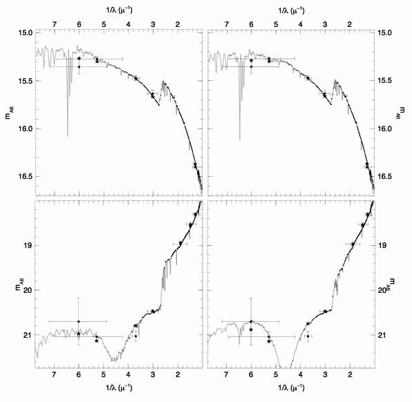
Figure 3: SEDs for the best fits of clusters I–As and I–Es, based on Starburst99 models of integrated stellar populations. The photometry is shown by the symbols with error bars (vertical ones for uncertainties and horizontal ones for the approximate length coverage of each filter.) Star symbols indicate the calculated magnitude of the model SED for each filter. [Top left] Best fit SED for cluster I–As using an LMC2–like extinction law. [Top right] Best fit SED for cluster I–As using an SMC–like extinction law. [Bottom left] Best fit SED for cluster I–Es for the old (189 Myr) solution. [Bottom right] Best fit SED for cluster I–Es for the young (7 Myr) solution.

Running the code with the same set of magnitudes, but constraining the extinction law to a MC–type (average LMC, LMC2, or SMC) we obtained similar values, as shown in Table 4. Since we are fitting two parameters and using four colors (derived from five magnitudes), the problem has 2 degrees of freedom. The best fit, which is certainly degenerate, appears to be the one obtained using the SMC extinction law, according to the $\chi^{2}$ reduced value. Figure 3 shows the SEDs that best agree with the data for the LMC2 and SMC fits. In Figure 4 we show the reddening vs. age likelihood contour plots using the LMC2 and SMC extinction laws. Both plots show that the age of this cluster spans the range $6.50\leq\log(\rm{age/yr})\leq 6.70$.

CHORIZOS provides a time–dependent correction that can be applied to transform the current magnitude of a cluster to the one at zero age. We used this quantity to derive the clusters zero age masses. For our analysis, we used Starburst99 models which only include stars more massive than $1\,M_{\odot}.$ Since most of a cluster’s mass is contained in the low–mass stellar population, we had to further correct these values considering a realistic IMF that spans the mass range $0.1-100\,M_{\odot}.$ All our mass estimates in this paper were therefore calculated using a Kroupa IMF (Kroupa, 2002) which considers stars in the range $0.1-100\,M_{\odot}.$

The derived mass of cluster I–As is $\approx 27\,000M_{\odot}.$ Once the approximate mass of the cluster was known, we used the Starburst99 output to calculate the stellar content of a cluster with this mass, an SMC–like metallicity $(Z=0.004)$ and the appropriate age. The results of the evolutionary synthesis models are shown in Table 4. It is known that cluster I–As is a SSC with a compact core and a strong massive halo, very similar in structure to 30 Doradus in the LMC, as shown by Maíz-Apellániz (2001). This implies that aperture effects are very important when performing any kind of photometric measurements for this cluster, and the derived quantities such as the mass of the cluster and the stellar population will depend on the chosen aperture.

Using an SMC extinction law, our models yield an age of $4.0\pm 0.6$ Myr for cluster I–As from the optical–UV photometry. This value agrees with the ones obtained by Leitherer et al. (1996) using UV spectroscopy (4–5 Myr) and by Maíz-Apellániz et al. (1998) using $W$(H$\beta$) and the strength of the WR 4660 Å blend (3–4 Myr). The models that best fit our data yield the values $A_{V}=0.19\pm 0.06,$ and $E(4405-5495)=0.04\pm 0.01$ mag . This low extinction is expected, since I–As is located within a heart–shaped H$\alpha$ cavity created by the kinetic energy input of the cluster into its surrounding medium (Maíz-Apellániz et al., 1999; MacKenty et al., 2000) and, therefore, one would expect little gas or dust in the line of sight. The quite large number of massive stars formed here have apparently wiped out the dust particles from their surroundings, leaving free paths through which the stellar continuum can emerge. The low extinction agrees with the value measured at this location by Maíz-Apellániz et al. (1998) from the nebular ratio of H$\alpha$ to H$\beta$.

From the detection of a broad emission feature from Wolf–Rayet stars (WRs), several authors (Leitherer et al., 1996; Sargent & Filippenko, 1991; Mas-Hesse & Kunth, 1991; Maíz-Apellániz et al., 1998) indicate the presence of WR stars inside cluster I–As. Leitherer et al. (1996) reexamined the results of Sargent & Filippenko (1991). Their results were calculated from ultraviolet spectra of cluster I–As obtained with the Faint Object Spectrograph onboard the HST in 1993. They used the $1\farcs 0$ circular aperture and assumed a distance of 4.1 Mpc to NGC 4214. They estimated that approximately 15 WN and 15 WC stars are present inside cluster I–As, keeping in mind uncertainties of a factor of 2. These results translate to 5 WR stars using the improved distance of 2.94 Mpc. Maíz-Apellániz et al. (1998) study four regions with WR stars in NGC 4214, including cluster I–As. Using their observed values of the equivalent widths of the WR blend we can estimate 60 WR stars inside an area of radius $1\farcs 8$ assuming a distance of 4.1 Mpc. This result is equivalent to 3 WR stars inside the aperture radius that we had used for cluster I–As at a distance of 2.94 Mpc. The CHORIZOS results predict 4 WRs using the same metallicity $(Z=0.020)$, and 1 WR using $(Z=0.004)$, which is consistent with the observations. It is important to note that WR stars may be present both in the nucleus of the cluster, and they may also be part of the massive halo. We want to emphasize that aperture effects are of great significance in dealing with this cluster. This makes it hard to compare different works performed with different techniques; however, our results are within Poisson errors of previous published values.

5.1.2 Cluster I–Es

We executed CHORIZOS for cluster I–Es using seven observed magnitudes (six colors) from Table 6 in Paper I and leaving all parameters unconstrained. The likelihood map produced by CHORIZOS  shows two solutions in the [$\log({\rm age})$, $E(4405-5495)$] plane, a young one around $\log({\rm age/yr})\approx 6.85$, and an old one around $\log({\rm age/yr})\approx 8.25$. We reran the code to isolate these two solutions using those age intervals, and the properties of both solutions are shown in Table 4. The old solution (age of $189\pm 53$ Myr) is the one that has the highest probability, but the young solution cannot be immediately rejected. The likelihood contour plots produced by CHORIZOS for this cluster are shown in Figure 5 for both solutions. The young solution shows very well defined ellipses in the plots. The old solution yields a high value of $R_{5495}$ which is clearly visible in Figure 5 (lower row, center and right.) The SED for both models are given in Figure 3. Both solutions show that cluster I–Es is older that cluster I–As which agrees with MacKenty et al. (2000) who indicate that the continuum colors of I–Es are significantly redder than for I–As, indicating a greater age. We executed Starburst99  to estimate the stellar content of a cluster with mass, age and metallicity appropiate for both solutions. The young solution ($\approx 6\,000M_{\odot}$ ) predicts the presence of 1 red supergiant and 2 blue supergiants, while the old solution ($\approx 129\,000M_{\odot}$ ) predicts 9 red supergiants and zero blue supergiants.

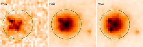
Figure 6: Images of cluster I–Es obtained with HST/WFPC2 using filters F336W, F555W, and F814W. The images have been resampled in order to use the same linear scale in all cases, with the field sizes being $15.9\times 15.9$ pc². The orientation in each case is north pointing up and east pointing to the left. Special attention must be drawn to the two objects located off center from the cluster. See the text for a complete discussion.

Trying to discern between the two possible solutions leads us to give a word of caution about the predictions of stellar synthesis models: in general, theoretical models have intrinsic uncertainties, especially when dealing with fast–evolving phases such as the RSG one. Furthermore, a more subtle effect is caused by incomplete sampling. Most current synthesis codes predict the average values of observables for an infinitely large population of stars, which samples a given IMF completely. Cerviño & Valls-Gabaud (2003) show that for an integrated property which originates from an effective number of stars $N$, there is a critical value of $N\approx 10$ below which the results of the codes must be taken with caution, since they can be biased and underestimate the actual dispersion of the observables. Cluster I–Es is an example of this sampling problem, since its F814W magnitude is dominated by the presence of a few RSGs (both the old and young solutions predict this). Therefore, the integrated colors are not enough to differentiate between the two solutions, since stochastic effects should be larger than evolutionary ones. Is there a way to overcome this issue? One could do it by looking at the resolved stellar population of the cluster, which is what we attempt in Figure 6 by representing cluster I–Es in detail in three filters: F336W, F555W, and F814W. A close inspection of these plots reveals that the cluster has some non–radial substructure. These images show two objects that blend with the structure of cluster I–Es, which are located inside the aperture radius that we used for the photometry marked in green in Figure 6. The object located towards the north is clearly visible in three filters (and is likely to be a BSG), while the other is not detectable in filter F336W (and is likely to be a RSG). The presence of a single bright red object favors the young solution over the old one, given that the first one predicts 1 RSG and the second one 9 of them. On the other hand, the bright red object could simply be a RSG unassociated with the cluster that happens to lie in the same direction (a look at Figure 2 shows that this possibility is not unlikely). Therefore, we have to conclude that the available data does not allow us to discern between the two solutions.

Regarding the extinction that affects I–Es, both solutions (young and old) yield values much higher than for I–As. This is consistent with the H$\alpha$/H$\beta$ results of Maíz-Apellániz et al. (1998) and Maíz-Apellániz (2000) and with the existence of a small peak in the CO distribution near the position of the cluster (Walter et al., 2001). Also, it is interesting to note that the $R_{5495}$ obtained from either solution is higher than the standard 3.1. However, given the uncertainty in the characteristics of this cluster deduced from its integrated colors caused by its relatively low number of stars, we should regard this measurement of $R_{5495}$ as rather uncertain.

5.1.3 Cluster IIIs

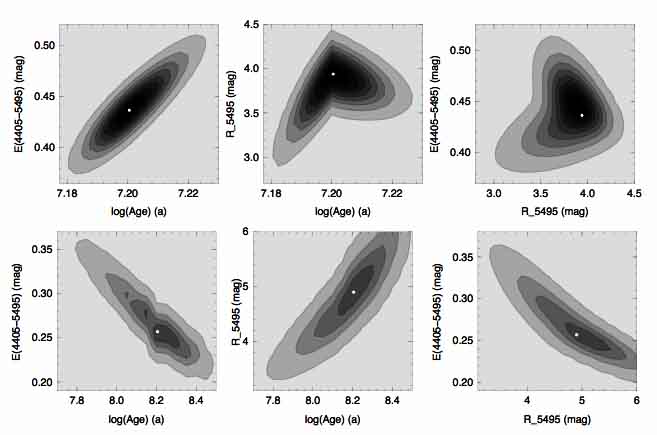
Figure 7: Likelihood contour plots for cluster IIIs provided as output by CHORIZOS and obtained using Starburst99 models. The upper row corresponds to the young solution and the lower row to the old one. [left] Reddening vs. age plot. [Center] Extinction law vs. age. [Right] Extinction law vs. reddening. Age is expressed in years. The white circle marks the most likely value (mode).

To analyze cluster IIIs, we used all seven magnitudes listed in Table 6 from Paper I. We executed CHORIZOS without limiting any parameter and using F336W as the reference filter. This gave us 7 magnitudes, 6 colors and 3 free parameters. We found an excellent fit of the spectrum with two possible solutions: a weak (high $\chi^{2}$) young solution around $\log({\rm age/yr})\approx 7.20$ and a stronger (low $\chi^{2}$) around $\log({\rm age/yr})\approx 8.20$. We reran the code twice to isolate these two solutions and the results for both models are presented in Table 4. The likelihood contour plots for both solutions are presented in Figure 7. Both solutions are very good fits, with small values of $\chi^{2}$. The slight difference between the two SEDs (Figure 8) lies in the depth of the bump located around 2175 Å.This spectroscopic feature is known as the graphite bump. Our study cannot disentangle between both solutions, since we do not have any measured magnitude in this part of the spectrum. However, the relative position of this cluster in the galaxy suggests that a low value of the extinction is to be expected. Also, the image of the cluster appears to be smooth, with no salient features throughout its structure. These two properties suggest that the old solution (age of $168\pm 61$ Myr, mass of $(6\pm 2)\times 10^{5}$ $M_{\odot}$ ) should be preferred over the young solution.

5.1.4 Cluster IVs

To analyze cluster IVs, we used all seven magnitudes listed in Table 6 from Paper I. We executed CHORIZOS without limiting any parameter and using F555W as the reference filter. There are two distinct solutions compatible with our set of magnitudes: a weak young solution around $\log({\rm age/yr})\approx 7.20$ and a more conspicuous old around $\log({\rm age/yr})\approx 8.20$. Figure 8 represents the best fit spectra for both solutions, and Figure 9 shows the probability contour plots for the young (upper row) and old (lower row) solutions. With our current magnitudes, it is not possible to decide between both models. However, for cluster IVs we expect a low value of the extinction since it is located in a region of the galaxy with little gas and dust. Also, as in cluster IIIs, its smooth appearence favors the old solution (age of $150\pm 34$ Myr) over the young model. As in cluster I–As, we find large values of $R_{5495}$ (spanning the range $2.0\leqslant R_{5495}\leqslant 6.0$), indicating that for a low value of the extinction, $R_{5495}$ is degenerated. In order to disentangle this problem, it would be useful to measure a magnitude near the right side of the Balmer discontinuity such as F439W (WFPC2 $B$).

In Table 4 we present the number of K+M stars of types I and II, obtained from Starburst99. It is noticeable that in clusters IIIs and IVs, the young solution provides a much lower quantity of RSGs than the old solution. The larger number of RSGs would explain the smooth appearance observed in the images, and this is another fact that favors the older solution for clusters IIIs, and IVs. Larsen et al. (2004) estimate $\sim(200\pm 52)$ Myr as the age of clusters IIIs and IVs, which is consistent with our results.

5.2 Resolved clusters

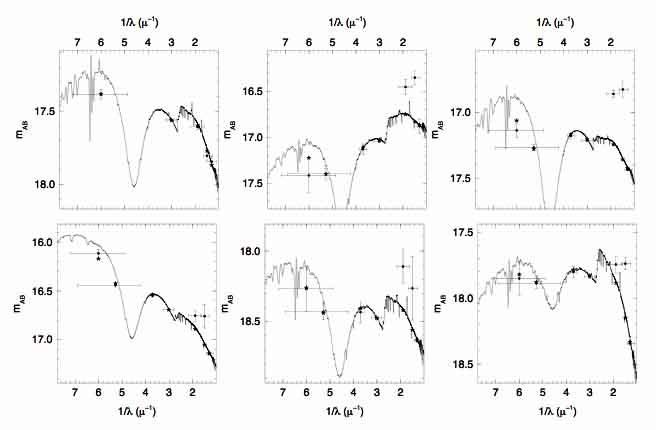
Figure 10: SEDs for the best fits of clusters I–Ds [Top–left], II–A [Top–center], II–B [Top–right], II–C [Bottom–left], II–D [Bottom–center], and II–E [Bottom–right], based on Starburst99 models of integrated stellar populations. The photometry is shown by the symbols with error bars (vertical ones for uncertainties and horizontal ones for the approximate length coverage of each filter.) Star symbols indicate the calculated magnitude of the model SED for each filter. Magnitudes in filters F555W and F702W are displayed in the spectrum of NGC 4214–IIABCDE, but they were not considered during the execution of CHORIZOS because of possible contamination.

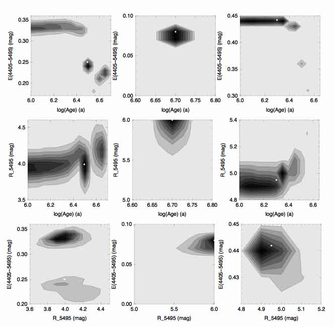
Figure 11: Likelihood contour plots for clusters I–Ds [Left], I–B [Middle], and II [Right] provided as output by CHORIZOS and obtained using Starburst99 models. [Top] Reddening vs. age plot. [Center] Extinction law vs. age. [Bottom] Extinction law vs. reddening. Age is expressed in years. The white circle marks the most likely value (mode).

We used five magnitudes from Table 7 in Paper I to execute CHORIZOS for cluster I–Ds. We left all parameters [ $\log({\rm age})$, $E(4405-5495)$, $R_{5495}$ ] unconstrained, which means that we had only one degree of freedom in this run. Figure 10 shows the best fit spectrum to the measured data. The contour plots for this cluster are presented in Figure 11 (left column.) There appears to be two possible solutions, both of them very young, with a strong peak at $\log({\rm age/yr})\approx 6.5$. The output of the code yields a mean age of $2.6\pm 1.5$ Myr, and a mean extinction of $E(4405-5495)=0.28\pm 0.05$ mag. The results are listed in Table 5.

The rest of the clusters which are part of the structure of complex II, were analyzed in a similar way. We used the set of magnitudes listed in Table 7 from Paper I with the exception of magnitudes F555W and F702W for the reason explained below. We obtain fairly good fits (highest $\chi^{2}=2.53$ ) which we display in Figure 10. Note that the points that correspond to magnitudes F555W and F702W are plotted, but they were not considered during the execution of CHORIZOS because those magnitudes are heavily contaminated by nebular emission.

The equivalent width of the Balmer lines can be used to estimate the age of a star–forming region (Cerviño & Mas-Hesse, 1994). The expected values for $W$(H$\alpha$) are $1000-2500$ Å for very young clusters (age $\lesssim 3$ Myr) and $500-1000$ Å for ages in the range between 3 and 4 Myr. MacKenty et al. (2000) estimated this parameter using three extinction corrections for all the clusters in NGC 4214.

The first execution for cluster II–A showed two possible solutions compatible with our data. One in the range $0.1\leqslant E(4405-5495)\leqslant 0.26$ (in mag) and the other in the range $0.26\leqslant E(4405-5495)\leqslant 0.6$ (in mag). We reran the code to isolate the solutions individually, and here, we present the diagrams corresponding to the second case only. MacKenty et al. (2000) provide values of $W$(H$\alpha$) for all the clusters within NGC 4214–II. These are close to or higher than $1000$ Å indicating a very young age of this complex. This fact led us to favor the solution with the highest $E(4405-5495)$. With this method we can restrict the age of this cluster to $3.1\pm 1.4$ Myr. This means that there may be WR stars within its structure. We also obtain a large value of $R_{5495}$, compatible to the one calculated for cluster II.

As for cluster II–B, the first execution showed two potential solutions with the same mean value of $R_{5495}$. We isolated a young and an old solution. Here we present the plots that correspond to the younger one. Following the same reasoning as for II–A, we favor the younger solution because high values of $W$(H$\alpha$) are measured in this region of the galaxy. This solution yields a very small age: $2.0\pm 0.8$ Myr.

The results of the best fits for the other three clusters are given in Table 5. Cluster II–C yields a single young solution, while II–D and II–E have more complicated outputs; however, their reddenings are very similar, as well as their $R_{5495}$ values.

5.3 Large complexes

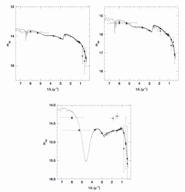
Figure 12: SEDs for the best fits of clusters I–A [Top–left], I–B [Top–right], and II [Bottom], based on Starburst99 models of integrated stellar populations. The photometry is shown by the symbols with error bars (vertical ones for uncertainties and horizontal ones for the approximate length coverage of each filter.) Star symbols indicate the calculated magnitude of the model SED for each filter. Magnitudes in filters F555W and F702W are displayed in the spectrum of NGC 4214–II, but they were not considered during the execution of CHORIZOS because of possible contamination. See text for details.

For complexes I–A, I–B, and II we ran CHORIZOS  leaving all three parameters [ $\log({\rm age})$, $E(4405-5495)$, $R_{5495}$ ] unconstrained. We used the estimated magnitudes from Table 6 in Paper I. Note that for complex II, magnitudes F555W and F702W are listed, but they were not considered for the $\chi^{2}-$fit. The inclusion of the 2MASS magnitudes did not change the output of the code significantly in any case. The best–fit SEDs are presented in Figure 12. The fits of complexes I–A, and I–B are excellent. The F170W magnitude is the one that contributes the most to $\chi^{2}=4.25$ in the case of cluster I–B. Figure 11 shows the contour plots provided as output by CHORIZOS for cluster I–B. It is clear from the plots that for cluster I–B there is a single solution compatible with our photometry. We obtain the same age (5.0 Myr) for both of them and, as expected, a low value for the extinction $E(4405-5495)=0.07$ mag. This value is very close to the one obtained for cluster I–As, as we had expected. It is important to note that the aperture that we used in both cases is large enough to include a part of the galaxy that contains a mixed population of stars. Figure 2 in Paper I clearly shows both late– and early–type stars are present within the apertures, something unexpected for an age of 5.0 Myr. Our extinction analysis showed that these large complexes contain stars with variable extinction as well. This leads to conclude that the SEDs for clusters I–A and I–B are composite spectra of different complex stellar populations. Again, the degeneracy in the extinction law for low values of the reddening gives high values or $R_{5495}$. An estimate of the total mass of these clusters gives: $(156\pm 19)\times 10^{3}$ $M_{\odot}$ for cluster I–A, and $(34\pm 4)\times 10^{3}$ $M_{\odot}$ for cluster I–B. All the results are presented in Table 6.

For cluster II we used the largest aperture radius: 200 PC pixels. This means that we are considering a mixed population of stars embedded in a gas–rich environment. As a result, we obtained a composite spectrum characterized by an age of $1.9\pm 0.9$ Myr. Its estimated mass is $(9\pm 3)\times 10^{5}$ $M_{\odot}$. The right column in Figure 11 shows the contour plots obtained for cluster II. The top plot indicates that this cluster is younger than cluster I–A, and that it is actually extinct. The middle and bottom diagrams imply that the law in the $R_{5495}$–dependent family of Cardelli et al. (1989) that best fits our photometry has a very high value or $R_{5495}$.

Complex II is expected to house objects with high extinction, since these are located within or very near filled H$\alpha$ regions that show little evidence of wind–blown or supernova created bubbles (Maíz-Apellániz et al., 1998; MacKenty et al., 2000). The extinction map represents very well this part of NGC 4214, showing the highest values of extinction in the southern part of cluster II–A and between clusters II–B and II–C. The measured values for the stellar $E(4405-5495)$ are in good agreement with those obtained from H$\alpha$/H$\beta$ (Maíz-Apellániz et al., 1998). We also calculated the mean value of the stellar extinction in each of the clusters (II–ABCDE) inside complex NGC 4214–II and found excellent agreement with the values obtained by fitting Starburst99 models to the spatially–integrated magnitudes. One remarkable result from Table 6 is that our models yield high values of $R_{5495}$ when we analyze large complexes. When using a large aperture one includes a mixed population of stars; we analyzed the $R_{5495}$ output for the brightest stars in this region and found that individual stars have indeed large values of extinction, specially those in cluster II–B. It is well known that the value of $R_{5495}$ depends upon the environment along the line of sight. A direction through low–density ISM usually has rather low value of extinction (about 3.1). Lines of sight penetrating into dense molecular clouds like Orion, Ophiuchus or Taurus yield $4<R_{V}<6$ (Mathis, 1990). For example, star Her 36 in M 8 has $R_{5495}=5.39\pm 0.09$ (Arias et al., 2006).

6 Summary and conclusions

6.1 Extinction

Using the estimated values of stellar extinction from the output of CHORIZOS, we built an extinction map in the field of view where we performed our study. The most noticeable characteristic in this map are the low values of the extinction scattered throughout the map, with the exception of some well defined regions with high values. We compared our extinction map with results provided by Maíz-Apellániz et al. (1998) and Maíz-Apellániz (2000) who used the Balmer ratio (H$\alpha$/H$\beta$) as a tracer of the reddening. They found that the reddening in NGC 4214–II is, on average, higher than in NGC 4214–I. Our results, derived from the stellar colors, are in agreement. The two main cavities in NGC 4214–I show low extinction surrounded by higher values while for NGC 4214–II the extinction is overall higher. Our extinction map traces fairly well the molecular clouds studied by Walter et al. (2001) which are directly associated to the star–forming regions in NGC 4214.

Studying the stellar content of seven blue compact galaxies, Fanelli et al. (1988) found a discrepancy between the extinction derived from the UV continuum of starburst galaxies and that derived from the Balmer lines. The extinction derived from UV continuum was systematically lower. Calzetti et al. (1994) analyzed $IUE$ UV and optical spectra of 39 starburst and blue compact galaxies in order to study the average properties of dust extinction. They derived the UV and optical extinction law under the hypothesis that the dust is a screen in front of the source. The characteristics of the extinction law are different from the MW and LMC laws: the overall slope is more gray than the MW or LMC slopes, and, most remarkably, the 2 175 Å dust feature is absent within the observational uncertainties. The different slope explained the differences observed between stellar and nebular extinction. However, Mas-Hesse & Kunth (1999) showed that the observed UV to optical SEDs of 17 starburst galaxies can be very well reproduced by reddening the corresponding synthetic spectra with one of the three extinction laws (Galactic, LMC, and SMC) with no need to invoke an additional universal law. As proposed by Mas-Hesse & Kunth (1999) and MacKenty et al. (2000), the effect was merely geometrical: while the continuum flux comes from the stars, the nebular emission originates in extended regions adjacent to the original molecular cloud. Stellar winds and supernova explosions might wipe out the dust from the neighborhood of the massive clusters and concentrate it in filaments and dust patches located within the ionizing region. Depending on the specific geometrical distribution of dust and stars, the extinction could affect mainly the nebular gas emission but only weakly the stellar continuum. This implies that the attenuation law by Calzetti et al. (1994) applies only to regions like I–A in NGC 4214, where the stars have evolved long enough to disrupt the ISM; meanwhile, this law should not be applied to NGC 4214–II, because the distribution of stars and dust are co–spatial in this part of the galaxy.

MacKenty et al. (2000) analyzed the differential extinction of the gas in NGC 4214 and found that once a cluster becomes older than $\approx 2$ Myr, the stellar components are mostly concentrated in those regions where the gas shows very low extinction. In our current work, we studied the differential extinction of the continuum from the stars in the galaxy. With this research we arrive to the conclusion that the extinction derived from the stellar continuum is similar to the extinction derived via the analysis of nebular lines across the galaxy, and we find this to be true on a pixel by pixel basis. The coincidence is fairly good throughout the galaxy. This confirms the idea advanced by Mas-Hesse & Kunth (1999) and MacKenty et al. (2000) that the differences between the Calzetti et al. (1994) attenuation law and other extinction laws are caused by the differences in the spatial distribution of the ionized gas and the young stellar population.

6.2 The ratio of blue–to–red supergiants

We approached the problem of determining the ratio of blue to red supergiants (B/R) in NGC 4214. We compared our observational results with three sets of theoretical models calculated with the MC metallicities and arrived at the conclusion that the best fit to our data is the non–rotating, $Z=0.004$, Geneva set (Maeder & Meynet, 2001). These models predict a B/R value of 24 in the $15-20\,M_{\sun}$ mass–range, and we measure $34\pm 10$. In the mass–range $20-25\,M_{\sun}$ the theoretical prediction is 47 and we obtain $46\pm 23$. In both cases, our results agree with the theoretical ones within Poisson errors. We discussed two caveats in the determination of B/R: the stochastic effects due to small–number statistics of RSGs in our sample in NGC 4214, and the conversion from observed colors to effective temperatures and bolometric magnitudes. We observe a discrepancy of $350-400$ K in our data which may be accounted for by fitting the observed optical colors using CHORIZOS or a similar code with MARCS atmospheres instead of Kurucz atmospheres.

6.3 The initial mass function

We studied the initial mass function of NGC 4214 following the method provided by Lequeux (1979) with several improvements, and taking into account four sources of systematic effects (incompleteness of the data, optimum bin size, mass diffusion, and unresolved multiple systems) presented by Maíz-Apellániz et al. (2005). We obtained a mean value of $\gamma=-2.83$ for the IMF slope of NGC 4214 in a continuous star–formation scenario. Since the correction for unresolved objects is uncertain (given the large distance to NGC 4214), and knowing that unresolved objects produce a systematic flattening of the IMF slope, we conclude that the real value of the slope would be steeper than $\gamma=-2.83$. We expect the “real” IMF slope to be shallower than the one provided by Chandar et al. (2005) ($\gamma=-3.5$) and steeper than our calculated value. Our estimation is closer to the one calculated by Mas-Hesse & Kunth (1999) ($\gamma=-3.0$) for the sum of field and clusters in NGC 4214. Some OB associations in the Magellanic Clouds and the Milky Way (Massey, 1998) have comparable values of the IMF slope to the one that we obtained for NGC 4214.

6.4 Clusters

We searched for the best fits of Starburst99 models to photometric colors of 13 clusters in NGC 4214. We chose four unresolved compact clusters, three large complexes and six small resolved clusters.

We find that the best models that are compatible with our data of cluster I–As are those with a MC–like extinction law. These models predict that cluster I–As is a young ($4.0\pm 0.6$ Myr) massive ($\approx 27\,000M_{\odot}$) star cluster with low ( $E(4405-5495)=0.04$ mag ) extinction. Our study is consistent with the presence of WR stars in this cluster, with a number close to the value previously obtained by Leitherer et al. (1996) and Maíz-Apellániz et al. (1998). MacKenty et al. (2000) estimated the equivalent widths of the Balmer lines $W$(H$\alpha$) using three extinction corrections for all the clusters in NGC 4214, in order to restrict the clusters ages. For clusters NGC 4214–I–A and I–B they estimate an age in the range between 4 and 5 Myr, which agrees with our photometric method. Their age estimate for cluster I–Ds is 7 Myr, while we obtain a much smaller value: $2.6\pm 1.5$ Myr. Cluster I–Es provides two very different solutions, but with the current data we prefer not to favor any of the solutions over the other.

MacKenty et al. (2000) find equivalent widths of H$\alpha$ very close or higher than 1000 Å for all the knots in NGC 4214–II, except for II–C, indicating that this large complex is very young. We consistently obtain very small ages for all the clusters within NGC 4214–II, including cluster II–C. The overall value of the $W$(H$\alpha$) for NGC 4214–II is quite lower than 1000 Å. MacKenty et al. (2000) explain that this may be due to the existence of an underlying population. They took this effect into account and estimated the value $2.5-3.0$ Myr for the age of cluster II. Our age estimate is $1.9\pm 0.9$ Myr which agrees with their value. The $W$(H$\alpha$) for NGC 4214–I is in general lower than those of for NGC 4214–II, and these authors suggest an average age in the range $3.0-4.0$ Myr for cluster I.

Our analysis for clusters IIIs and IVs includes six photometric colors covering wavelengths from the UV to the IR. This allowed us to find restrictions to the age and mass of these clusters. Using several arguments (extinction values, number of red supergiants, image appearance) we suggest that the older solutions should be preferred over the younger ones in the case of these two clusters. Billett et al. (2002) study clusters IIIs and IVs as part of a survey of compact star clusters in nearby galaxies which include NGC 4214. Unfortunately, their aperture photometry includes errors such as not taking into consideration the contamination effect for filter F336W and the conversion of HST flight magnitudes to the Johnson–Cousins system, which is not recommended because of their limited precision (Gonzaga, 2003; de Grijs et al., 2005). Using an evolutionary track taken from the Starburst99 models on a color–color diagram, they infer age estimates to these clusters. The evolutionary track on this diagram is clearly degenerate, and shows several possible solutions for the age of these clusters. They used only two photometric colors, and this translates into a very poor determination of the clusters age (de Grijs et al., 2003b). Using the photometry produced by Billett et al. (2002) and the cluster evolutionary models of Bruzual & Charlot (2003), Larsen et al. (2004) infer the age and mass of clusters IIIs and IVs. The mass is inferred using a dynamical method for clusters in virial equilibrium.

We find that NGC 4214–IIIs and –IVs are compact old massive clusters with age $>100$ Myr. Ten other clusters (one unresolved compact cluster, three large complexes and six small resolved clusters) yield ages $<10$ Myr. Cluster luminosity functions and color distributions are the most important tools in the study of cluster populations in nearby galaxies. The use of individual cluster spectroscopy, acquired with 8–m–class telescopes is very time consuming, because observations of large numbers of clusters are needed in order to obtain statistically significant results. Multipassband imaging is a useful alternative. de Grijs et al. (2003b) analyze the systematic uncertainties in age, extinction, and metallicity determinations for young stellar clusters, inherent to the use of broad–band, integrated colors. They studied clusters within NGC 3310 and found that red–dominated passband combinations result in significantly different age solutions, while blue–selected passband combinations tend to result in age estimates that are slightly skewed towards lower ages. Their advise is to use at least four filters including both blue and red optical passbands. This choice leads to the most representative age distribution. See also Anders et al. (2004) and de Grijs et al. (2005).

For our cluster analysis in NGC 4214, we employed at least five filters in each case, and we determined all the free parameters individually for each cluster as suggested by de Grijs et al. (2003a). The accuracy to which the ages can be estimated depends on the number of different broad–band filters and, crucially, on the actual wavelengths range covered by the observations. We found some degeneracies that could have been disentangled, provided that we had a measurement of a magnitude near the right side of the Balmer discontinuity such as F439W (WFPC2 $B$). However, we are confident with the age estimate of our sample of clusters in NGC 4214.

Employing multicolor images of the Antennae galaxies, Fall et al. (2005) studied the age distribution of the population of star clusters. They estimated the cluster ages, by fitting SEDs from the Bruzual & Charlot (2003) models and found the age distribution declines steeply, starting at very young ages. The median age of the clusters is $\sim 10$ Myr. According to their study, after $\sim 10$ Myr, the surface brightness of the clusters would be 5 mag fainter than initially (at $\sim 1$ Myr), and therefore the cluster would disappear among the statistical fluctuations in the foreground and background of field stars. They call this effect the “infant mortality” of clusters. Our sample of clusters in NGC 4214 includes 10 objects younger than 10 Myr, with NGC 4214–IA and –IB already showing effects of disruption. What could cause the disruption of the clusters? Fall et al. (2005) claim that the momentum output from massive stars comes in the form of ionizing radiation, stellar winds, jets, and supernovae, and all these processes could easily remove much of the ISM from the protocluster leaving the stars within it gravitationally unbound. Another explanation is provided by Clark et al. (2005) who performed simulations and showed that unbound giant molecular clouds manage to form a series of star clusters and disperse in $\sim 10$ Myr, making them transient features. At later ages they would not be recognized as clusters. This result is further confirmed by several empirical and theoretical studies. See Lada & Lada (2003) for a review and the references therein. Lamers et al. (2005) present a simple analytical description of the disruption star clusters in a tidal field, and found that about half of the clusters in the solar neighborhood become unbound within about 10 Myr.

6.5 Implications

Nearby galaxies provide ideal laboratories to test how stars form, how star formation is triggered, and details of how galaxies assembled. The study of nearby galaxies like NGC 4214 is rather important because most of the information that we infer about high–redshift galaxies relies on what we observe in galaxies in the local universe. Therefore, understanding nearby galaxies is of extreme importance to comprehend what is going on in more distant ones. NGC 4214 is a low–metallicity galaxy, and this gave us the possibility to study the physical conditions in an environment of current astrophysical interest. In particular, we could infer that the B/R supergiant ratio is close to the one of the SMC and that its IMF is steeper that Salpeter.

Table 1: Comparison between theoretical and observational values of the ration B/R of the number of blue supergiants and red supergiants.

	SMC $v_{ini}\tablenotemark{a}=0$		SMC $v_{ini}=300$		LMC $v_{ini}=0$
mass range	theory	obs	theory	obs	theory	obs
$15-20$	24	$34\pm 10$	0.4	$29\pm 10$	1.0	$13\pm 4$
$20-25$	47	$46\pm 23$	0.4	$45\pm 31$	2.7	$67\pm 66$

Table 2: IMF slope values with their errors for the three lists calculated for several values of the low–mass end ($M_{low}$) and $M_{up}=100M_{\odot}$. These results would apply to a continuous star–formation region.

	I–A + I–B + II				Other regions				NGC 4214
$M_{low}[M_{\odot}]$	$\gamma_{fit}$	$\gamma_{real}$	$N$		$\gamma_{fit}$	$\gamma_{real}$	$N$		$\gamma_{fit}$	$\gamma_{real}$	$N$
15	-2.17	$-2.67\pm 0.08$	752		-2.15	$-2.64\pm 0.06$	1680		-2.15	$-2.64\pm 0.05$	2432
16	-2.20	$-2.61\pm 0.09$	655		-2.28	$-2.72\pm 0.06$	1494		-2.26	$-2.70\pm 0.05$	2149
17	-2.24	$-2.60\pm 0.10$	573		-2.43	$-2.83\pm 0.07$	1357		-2.39	$-2.78\pm 0.06$	1930
18	-2.21	$-2.51\pm 0.10$	501		-2.59	$-2.95\pm 0.08$	1216		-2.48	$-2.82\pm 0.06$	1717
19	-2.30	$-2.57\pm 0.11$	449		-2.72	$-3.03\pm 0.08$	1098		-2.56	$-2.86\pm 0.06$	1547
20	-2.36	$-2.60\pm 0.12$	397		-2.71	$-2.98\pm 0.09$	961		-2.58	$-2.83\pm 0.07$	1358

Table 3: IMF slope values with their errors for regions I–A, I–B, and II. These results would apply to a burst star–formation region.

		I–A + I–B + II
$M_{low}[M_{\odot}]$	$M_{up}[M_{\odot}]$	$\gamma_{fit}$	$\gamma_{real}$	$N$
15	100	-3.30	$-4.41\pm 0.09$	752
16	100	-3.25	$-4.06\pm 0.10$	655
17	100	-3.24	$-3.87\pm 0.10$	573
18	100	-3.14	$-3.61\pm 0.11$	501
19	100	-3.20	$-3.59\pm 0.12$	449
20	100	-3.23	$-3.56\pm 0.13$	397
40	100	-2.89	$-2.97\pm 0.37$	85
20	40	-3.73	$-4.41\pm 0.28$	312

Table 4: Results from CHORIZOS fitting for clusters I–As, I–Es, IIIs, and IVs. The mass was estimated using a Kroupa IMF (Kroupa, 2002). The number of stars is obtained from Starburst99 models.

Parameter	Cluster I–As			Cluster I–Es			Cluster IIIs			Cluster IVs
	LMC2	SMC		Young	Old		Young	Old		Young	Old
Age (Myr)	$4.0\pm 0.6$	$4.2\pm 0.6$		$7.1\pm 0.1$	$189\pm 53$		$15.8\pm 0.2$	$168\pm 61$		$15.8\pm 0.0$	$150\pm 34$
$E(4405-5495)$ (mag)	$0.05\pm 0.01$	$0.04\pm 0.01$		$0.46\pm 0.01$	$0.32\pm 0.03$		$0.44\pm 0.01$	$0.26\pm 0.03$		$0.22\pm 0.01$	$0.06\pm 0.03$
Extinction law / $R_{5495}$	LMC2	SMC		$4.21\pm 0.25$	$5.72\pm 0.26$		$3.95\pm 0.20$	$4.98\pm 0.60$		$3.39\pm 0.52$	$4.35\pm 1.12$
Mass ($10^{3}M_{\odot}$)	$27\pm 4$	$27\pm 4$		$6\pm 1$	$129\pm 26$		$134\pm 18$	$626\pm 175$		$27\pm 4$	$114\pm 20$
$\chi^{2}$ per degree of freedom	1.33	0.91		2.58	2.19		0.39	0.66		1.77	2.18
O+B stars, types I and II	11	11		2	0		31	0		7	0
K+M stars, types I and II	0	0		1	9		6	45		1	26
WR stars	1	1		0	0		0	0		0	0

Table 5: Results from CHORIZOS fitting for resolved clusters.The mass was estimated using a Kroupa IMF (Kroupa, 2002).

Parameter	Cluster I–Ds	Cluster II–A	Cluster II–B	Cluster II–C	Cluster II–D	Cluster II–E
Age (Myr)	$2.6\pm 1.5$	$3.1\pm 1.4$	$2.0\pm 0.8$	$1.7\pm 0.6$	$4.0\pm 4.0$	$3.1\pm 1.4$
$E(4405-5495)$ (mag)	$0.28\pm 0.05$	$0.35\pm 0.08$	$0.35\pm 0.01$	$0.28\pm 0.01$	$0.22\pm 0.16$	$0.20\pm 0.05$
Extinction law / $R_{5495}$	$4.05\pm 0.19$	$3.79\pm 0.33$	$4.11\pm 0.11$	$4.82\pm 0.13$	$4.05\pm 0.91$	$2.92\pm 0.43$
Mass ($10^{3}M_{\odot}$)	$20\pm 9$	$34\pm 23$	$43\pm 10$	$63\pm 14$	$7\pm 5$	$7\pm 3$
$\chi^{2}$ per degree of freedom	1.31	0.41	2.02	2.53	0.15	0.22

Table 6: Results from CHORIZOS fitting for large complexes.The mass was estimated using a Kroupa IMF (Kroupa, 2002).

Parameter	Cluster I–A	Cluster I–B	Cluster II
Age (Myr)	$5.0\pm 0.0$	$5.0\pm 0.0$	$1.9\pm 0.9$
$E(4405-5495)$ (mag)	$0.07\pm 0.01$	$0.07\pm 0.01$	$0.43\pm 0.03$
Extinction law / $R_{5495}$	$5.88\pm 0.16$	$5.81\pm 0.19$	$4.99\pm 0.11$
Mass ($10^{3}M_{\odot}$)	$156\pm 19$	$34\pm 4$	$923\pm 331$
$\chi^{2}$ per degree of freedom	0.95	4.25	0.21

References

- Anders et al. (2004) Anders, P., Bissantz, N., Fritze-v. Alvensleben, U., & de Grijs, R. 2004, MNRAS, 347, 196
- Annibali et al. (2003) Annibali, F., Greggio, L., Tosi, M., & Leitherer, C. 2003, AJ, 126, 2752
- Arias et al. (2006) Arias, J. I., Barbá, R. H., Apellániz, J. M., Morrell, N. I., & Rubio, M. 2006, MNRAS, 366, 739
- Billett et al. (2002) Billett, O. H., Hunter, D. A., & Elmegreen, B. G. 2002, AJ, 123, 1454
- Brunish et al. (1986) Brunish, W. M., Gallagher, J. S., & Truran, J. W. 1986, AJ, 91, 598
- Bruzual & Charlot (2003) Bruzual, G. & Charlot, S. 2003, MNRAS, 344, 1000
- Calzetti et al. (2004) Calzetti, D., Harris, J., Gallagher, J. S., Smith, D. A., Conselice, C. J., Homeier, N., & Kewley, L. 2004, AJ, 127, 1405
- Calzetti et al. (1994) Calzetti, D., Kinney, A. L., & Storchi-Bergmann, T. 1994, ApJ, 429, 582
- Cardelli et al. (1989) Cardelli, J. A., Clayton, G. C., & Mathis, J. S. 1989, ApJ, 345, 245
- Cerviño & Valls-Gabaud (2003) Cerviño, M. & Valls-Gabaud, D. 2003, MNRAS, 338, 481
- Cerviño & Mas-Hesse (1994) Cerviño, M. & Mas-Hesse, J. M. 1994, A&A, 284, 749
- Chandar et al. (2005) Chandar, R., Leitherer, C., Tremonti, C. A., Calzetti, D., Meurer, G. R., & de Mello, D. 2005, ApJ, 628, 210
- Clark et al. (2005) Clark, P. C., Bonnell, I. A., Zinnecker, H., & Bate, M. R. 2005, MNRAS, 359, 809
- de Grijs et al. (2005) de Grijs, R., Anders, P., Lamers, H. J. G. L. M., Bastian, N., Fritze-v. Alvensleben, U., Parmentier, G., Sharina, M. E., & Yi, S. 2005, MNRAS, 359, 874
- de Grijs et al. (2003a) de Grijs, R., Bastian, N., & Lamers, H. J. G. L. M. 2003a, MNRAS, 340, 197
- de Grijs et al. (2003b) de Grijs, R., Fritze-v. Alvensleben, U., Anders, P., Gallagher, J. S., Bastian, N., Taylor, V. A., & Windhorst, R. A. 2003b, MNRAS, 342, 259
- de Vaucouleurs et al. (1991) de Vaucouleurs, G., de Vaucouleurs, A., Corwin, H. G., Buta, R. J., Paturel, G., & Fouque, P. 1991, Third Reference Catalogue of Bright Galaxies (Volume 1-3, XII, 2069 pp. 7 figs.. Springer-Verlag Berlin Heidelberg New York)
- de Wit et al. (2004) de Wit, W. J., Testi, L., Palla, F., Vanzi, L., & Zinnecker, H. 2004, A&A, 425, 937
- Dohm-Palmer & Skillman (2002) Dohm-Palmer, R. C. & Skillman, E. D. 2002, AJ, 123, 1433
- Drozdovsky et al. (2002) Drozdovsky, I. O., Schulte-Ladbeck, R. E., Hopp, U., Greggio, L., & Crone, M. M. 2002, AJ, 124, 811
- Eggenberger et al. (2002) Eggenberger, P., Meynet, G., & Maeder, A. 2002, A&A, 386, 576
- Fall et al. (2005) Fall, S. M., Chandar, R., & Whitmore, B. C. 2005, ApJ, 631, L133
- Fanelli et al. (1988) Fanelli, M. N., O’Connell, R. W., & Thuan, T. X. 1988, ApJ, 334, 665
- Flower (1996) Flower, P. J. 1996, ApJ, 469, 355
- Garmany et al. (1982) Garmany, C. D., Conti, P. S., & Chiosi, C. 1982, ApJ, 263, 777
- Georgiev et al. (1999) Georgiev, L., Borissova, J., Rosado, M., Kurtev, R., Ivanov, G., & Koenigsberger, G. 1999, A&AS, 134, 21
- Gonzaga (2003) Gonzaga, S. 2003, WFPC2 Data Analysis: A Tutorial, version3.0 (STScI)
- González Delgado & Pérez (2000) González Delgado, R. M. & Pérez, E. 2000, MNRAS, 317, 64
- Gordon & Clayton (1998) Gordon, K. D. & Clayton, G. C. 1998, ApJ, 500, 816
- Gustafsson et al. (1975) Gustafsson, B., Bell, R. A., Eriksson, K., & Nordlund, A. 1975, A&A, 42, 407
- Humphreys (1983) Humphreys, R. M. 1983, ApJ, 265, 176
- Humphreys & McElroy (1984) Humphreys, R. M. & McElroy, D. B. 1984, ApJ, 284, 565
- Humphreys & Sandage (1980) Humphreys, R. M. & Sandage, A. 1980, ApJS, 44, 319
- Hunter (2001) Hunter, D. A. 2001, ApJ, 559, 225
- Jamet et al. (2004) Jamet, L., Pérez, E., Cerviño, M., Stasińska, G., González Delgado, R. M., & Vílchez, J. M. 2004, A&A, 426, 399
- Kroupa (2002) Kroupa, P. 2002, Science, 295, 82
- Kroupa et al. (1991) Kroupa, P., Gilmore, G., & Tout, C. A. 1991, MNRAS, 251, 293
- Kurucz (2004) Kurucz, R. L. 2004, in http://kurucz.harvard.edu
- Lada & Lada (2003) Lada, C. J. & Lada, E. A. 2003, ARA&A, 41, 57
- Lamers et al. (2005) Lamers, H. J. G. L. M., Gieles, M., Bastian, N., Baumgardt, H., Kharchenko, N. V., & Portegies Zwart, S. 2005, A&A, 441, 117
- Langer & Maeder (1995) Langer, N. & Maeder, A. 1995, A&A, 295, 685
- Larsen et al. (2004) Larsen, S. S., Brodie, J. P., & Hunter, D. A. 2004, AJ, 128, 2295
- Leitherer et al. (1999) Leitherer, C., Schaerer, D., Goldader, J. D., Delgado, R. M. G., Robert, C., Kune, D. F., de Mello, D. F., Devost, D., & Heckman, T. M. 1999, ApJS, 123, 3
- Leitherer et al. (1996) Leitherer, C., Vacca, W. D., Conti, P. S., Filippenko, A. V., Robert, C., & Sargent, W. L. W. 1996, ApJ, 465, 717
- Lejeune & Schaerer (2001) Lejeune, T. & Schaerer, D. 2001, A&A, 366, 538
- Lequeux (1979) Lequeux, J. 1979, A&A, 80, 35
- Levesque et al. (2005) Levesque, E. M., Massey, P., Olsen, K. A. G., Plez, B., Josselin, E., Maeder, A., Meynet, G., & White, N. 2005, ApJ, 628, 973
- MacKenty et al. (2000) MacKenty, J. W., Maíz-Apellániz, J., Pickens, C. E., Norman, C. A., & Walborn, N. R. 2000, AJ, 120, 3007
- Maeder & Meynet (2001) Maeder, A. & Meynet, G. 2001, A&A, 373, 555
- Maíz-Apellániz (2001) Maíz-Apellániz, J. 2001, ApJ, 563, 151
- Maíz-Apellániz (2004) —. 2004, PASP, 116, 859
- Maíz-Apellániz et al. (2002) Maíz-Apellániz, J., Cieza, L., & MacKenty, J. W. 2002, AJ, 123, 1307