The young stellar population of NGC 4214 as observed with HST. I. Data and methods.

Abstract

We present the data and methods that we have used to perform a detailed UV–optical study of the nearby dwarf starburst galaxy NGC 4214 using multifilter HST/WFPC2+STIS photometry. We explain the process followed to obtain high–quality photometry and astrometry of the stellar and cluster populations of this galaxy. We describe the procedure used to transform magnitudes and colors into physical parameters using spectral energy distributions. The data show the existence of both young and old stellar populations that can be resolved at the distance of NGC 4214 (2.94 Mpc) and we perform a general description of those populations.

1 Introduction

NGC 4214 is a nearby dwarf IAB(s)m galaxy (de Vaucouleurs et al., 1991) in the low–redshift CVn I Cloud (Sandage & Bedke, 1994) located at a distance of $2.94\pm 0.18$ Mpc (Maíz-Apellániz et al., 2002). The galaxy is moderately metal–deficient (Kobulnicky & Skillman, 1996) with $12+\log(\mathrm{O/H})$ between $8.15$ and $8.28$. The optical nebular morphology of NGC 4214 (MacKenty et al., 2000) shows three differentiated components: (1) two large H II star–forming complexes, known in the literature as NGC 4214–I (or NW complex) and NGC 4214–II (or SE complex); (2) a number of isolated fainter knots scattered throughout the field; (3) an extended, structurally amorphous, Diffuse Interstellar Gas (DIG) surrounding the two main complexes and some of the isolated knots; see Figure 1. The individual H$\alpha$ knots have been identified by several authors in the past and MacKenty et al. (2000) have provided a more standardized nomenclature with 13 different units, which we adopt for this work.

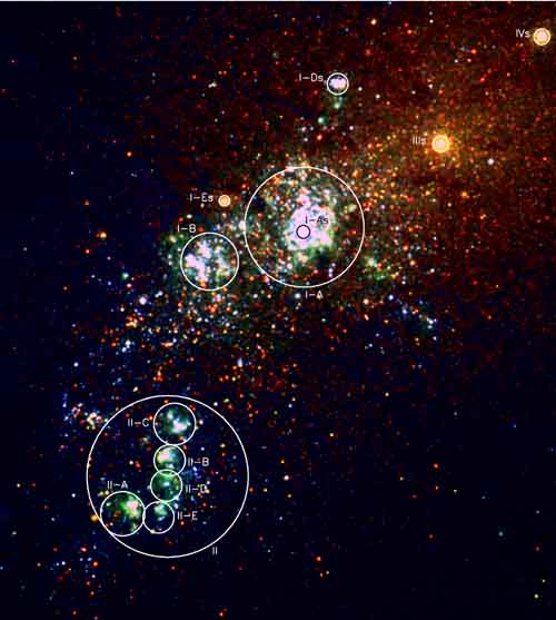
Figure 2: Mosaic of NGC 4214 obtained using images in filter F336W (blue), F555W  (green), and F814W  (red). We show and label the cluster circular apertures. The orientation is north pointing up and east pointing to the left. The field dimensions are 875 pc $\times$ 972 pc or $61\farcs 4\times 68\farcs 3$.

What follows is a summary of this galaxy’s morphology. Refer to Figure 2 for guidance. NGC 4214–I is the largest H II complex in the galaxy and the one with the most intricate morphology. It includes several star clusters and has a complex H$\alpha$ structure dominated by the presence of two cavities or intensity minima. I–As is a massive young Super Star Cluster (SSC) located off–center in a heart–shaped H$\alpha$ cavity. The H$\alpha$ emission surrounding I–As consists of a number of knots joined by filaments. I–Bs is a scaled OB association (or SOBA, Hunter 1999, Maíz-Apellániz 2001): a massive cluster that, as opposed to an SSC, does not show a marked central concentration. I–Bs is also located in the middle of an elongated H$\alpha$ cavity, though not as clearly defined as the I–As one. NGC 4214–II is the second largest complex in the galaxy (in angular size) and harbors the regions with the highest peak H$\alpha$ intensity. Its morphology is quite different from that of NGC 4214–I. In the first place, there is no dominant SSC but several smaller clusters which are responsible for the ionization of the gas. Also, there are no large cavities present and the clusters are located very close to (or at the same position as) the most intensely H$\alpha$ emitting knots (Maíz-Apellániz et al. 1998). II–A and II–B are the two brightest H$\alpha$ knots in NGC 4214–II. They are both located on top of clusters which, at the resolution of WFPC2, appear to be centered at the same positions. NGC 4214–IIIs is a compact continuum source with weak associated H$\alpha$ emission. It is either an older cluster or the nucleus of the galaxy, as suggested by the study of Fanelli et al. (1997) in the I band and the FUV. NGC 4214–IVs has a similar appearance to NGC 4214–IIIs and it is probably another intermediate-age massive cluster. MacKenty et al. (2000) provides a more detailed description.

The high intensity of the recent star and cluster formation rate in NGC 4214 combined with its proximity and its low foreground extinction make this galaxy an excellent target to test several subjects of astrophysical interest regarding young stellar populations. Nearby galaxies, and in particular NGC 4214, provide ideal laboratories to test how stars form, how star formation is triggered, and details of how galaxies assembled. The study of nearby galaxies like NGC 4214 is rather important because most of the information that we infer about high–redshift galaxies relies on what we observe in galaxies in the local universe. Therefore, understanding nearby galaxies is of extreme importance to comprehend what is going on in more distant ones. NGC 4214 is a low–metallicity galaxy, and this gave us the possibility to study the physical conditions in an environment of current astrophysical interest.

In this paper we present the data and the methods that we used to analyze it. We have built detailed photometric lists with the most accurate astrometry. Of particular interest is the new IDL code (Maíz-Apellániz, 2004) that we used to transform observed magnitudes and photometric colors into actual stellar and cluster physical parameters. We also make a brief description of its stellar population.

In the accompanying paper [(Úbeda et al., 2007), hereafter Paper II] we will study the ratio of blue to red (B/R) supergiants, the initial stellar mass function (IMF), the variable extinction across the galaxy, and the properties of its young– and intermediate–age cluster populations. This division is needed due to the vast amount of data and results that we have gathered, and to the intricate structure of the object of study: NGC 4214 presents a number of clusters in different stages of evolution, individually resolved stars, and several regions of star formation, characterized by the presence of complex nebulosities. H II regions of different morphology can be clearly seen in our images, showing the distinct nature of this interesting galaxy.

The present paper is organized as follows: In Section 2 we provide a description of our observations and data reduction, with emphasis on the creation of the photometric lists and the consistency tests. In Section 2.5 we introduce the method used to translate the observed magnitudes and colors into physical parameters. In Section 3 we provide a general description of the stellar populations visible in our images. A brief summary is provided in Sections 4.

2 Observations and data reduction

2.1 WFPC2 Observations and reduction

Wide Field and Planetary Camera 2 (WFPC2) is a two-dimensional imaging photometer which consists of three CCD cameras (WF) with a spatial sampling of $0\farcs 1$ per pixel and a smaller CCD camera (PC) with $0\farcs 046$ per pixel.

The WFPC2 images were acquired in two programs: 6569 (P.I.: John MacKenty) and 6716 (P.I.: Theodore Stecher). Figure 1 shows the location of the WFPC2 fields for the programs that we have used. All images include complexes NGC 4214–I and NGC 4214–II. Table 1 lists all the NGC 4214 WFPC2 data that we have used for this paper. The images available in each program can be summarized as follows: 6716, UV and $UVI$; 6569, narrow–band ([O III] $\lambda$5007, and H$\alpha$) + broad–band $UVI$. The WFPC2 observations of program 6569 were obtained on 22 July 1997, and those of program 6716 were obtained on 29 June and 9 December 1997. For proposal 6569, the pointing of the telescope was chosen in order to minimize charge transfer efficiency (CTE) effects, since in this way no area of interest was separated from its collecting point by low signal areas (MacKenty et al., 2000). In the case of proposal 6716, the location was chosen in order to capture the most interesting regions of NGC 4214 with the PC, a camera that provides a higher resolution. These images allow us to obtain accurate single star photometry not easily achievable from the ground due to the very complex diffuse emission and crowding.

The standard WFPC2 pipeline process takes care of the basic data reduction (bias, dark, flat–field corrections). The reduction of the processed frames was performed using the PSF–fitting package HSTphot (Dolphin, 2000), which yielded calibrated magnitudes in the VEGAMAG system corrected for charge–transfer efficiency (CTE) for all filters. We ran HSTphot twice: first using a flag that estimates the sky locally, and later using the flag that refits the sky during photometry. In both runs we used the default aperture corrections for each filter provided by HSTphot. The adopted magnitude for each star is the mean obtained from the two executions, and the errors in the magnitudes were estimated from the internal errors in each run. The consistency of the photometry is analyzed in Section 2.3.

The WFPC2 CCD windows suffer from a time–dependent contamination which primarily affects UV observations and is negligible at optical wavelengths. The contaminants are largely removed during periodic warmings (decontaminations) of the camera, and the effect upon photometry is both linear and stable and can be removed using values regularly measured in the WFPC2 calibration program (McMaster & Whitmore, 2002). We performed contamination correction for images obtained with filters F170W and F336W. The presence of saturated objects was analyzed in all the images, and we found that cluster I–As appears saturated in filter F555W of proposal 6716 and in filters F336W, F555W, and F702W of proposal 6569. Cluster IIIs appears saturated in all images obtained using filter F555W. In Section 2.4 we explain how we obtained the magnitudes for these clusters.

2.1.1 Astrometry

The geometric distortion of the WFPC2 detectors is well known (Casertano & Wiggs, 2001), allowing for precise relative astrometry. However, the absolute astrometry has two problems: First, the Guide Star Catalog, which is used as a reference on board Hubble Space Telescope, has typical errors of $\sim 1\arcsec$ (Russell et al., 1990). Second, if only one point in one of the four WFPC2 chips can be established as a precise reference using an external catalog, the average error in the orientation induces an error of $\sim 0\farcs 03$ in a typical position in the other three chips. In our case, two objects which are present in the WFPC2 fields are included in the USNO–A2.0 catalog as entries 1200–06870167 and 1200–06870199. We used the VizieR service (Ochsenbein et al., 2000) to obtain their coordinates using the J2000 epoch and equinox, and we adopted object 1200–06870167 as the astrometric reference point. This star is located in the center of region VIn which lies outside our studied field but which can be clearly seen in Figure 2 in MacKenty et al. (2000). 1200–06870199 is located in a very crowded region filled with many objects in our high resolution images, and therefore, its coordinates correspond to a blend of point sources, making it useless for our purposes. The procedure that we followed to establish a uniform coordinate system had three steps: First, we corrected for the difference in plate scale for each filter with respect to F555W using the parameters provided by Dolphin (2000) (note that the tasks mosaic and metric within the IRAF/STSDAS package, use the non–wavelength–dependent Holtzmann solution, which can introduce $\sim 0\farcs 1$ errors for FUV data; errors are up to an order of magnitude smaller if only optical data are involved). Second, we corrected for the geometrical distortion and built mosaics of the four WFPC2 fields using the mosaic utility, which is included in the standard STSDAS package for WFPC2 data analysis. We rotated all mosaiced images in order to make them share a common orientation, keeping in mind that this contributes to the astrometric accuracy due to subpixel rebinning. Third, using 1200–06870167 as a reference object, we corrected for the general displacement in right ascension and declination and compared the positions of the stars of several regions of NGC 4214 using images obtained under different filters. As expected, coordinates differed by a few hundredths of an arcsecond, which we take to be the precision of our absolute astrometry.

2.1.2 Cross–correlation

The field–of–view used for our analysis is shown in Figure 2 and its dimensions are: 875 pc $\times$ 972 pc or $61\farcs 4\times 68\farcs 3$. The region of the galaxy depicted by our field–of–view is clearly the most interesting one to study, because it includes the most prominent star–forming regions, as well as some clusters of importance. This field–of–view represents the overlapping section of several images obtained with HST/WFPC2 and HST/STIS (see next section).

The last step in the data reduction, the registration of the images obtained under different programs, was somewhat complicated. We developed custom–made IDL scripts which allowed us to cross–identify stars in the different bandpasses by positional matching. In order to join the lists obtained in different filters, we built two main photometric lists using F336W and F814W as reference filters. The lists are referred to here as LIST336 and LIST814. Even though the individual lists used in the cross–correlation were obtained with the same instrument, the orientation of the cameras was different for each list and the resolution and S/N used to image each object was also different. To combine the final proposal–6569 list with the final proposal–6716 list with filter F336W as reference, we used a cross–correlation procedure with the following characteristics: In the most crowded regions in our images (NGC 4214–I) we only considered objects from proposal 6716 because these images have a higher resolution. Outside that region, the cross–correlation could yield several cases: (a) an object found in proposal 6569 but not found in proposal 6716, (b) an object found in both proposals, (c) an object found in proposal 6569 that corresponds to two or more objects in proposal 6716. Our final list included all objects in case (a); if the object fell in case (b), we would consider the data from proposal 6569 due to its higher S/N, and get rid of its companion from proposal 6716. Finally, if the object fell in case (c) we would consider those objects from proposal 6716 due to the higher resolution of the PC and get rid of its companion from proposal 6569. With all the objects that were not correlated, we built another list using filter F814W as reference. LIST336 has 14 389 objects and LIST814 has 21 614 objects. Both lists of objects (LIST336 and LIST814) are available in the electronic edition of this paper. Tables 2 and 3 contain the first five lines of those lists as a sample. The tables include the equatorial coordinates ($\alpha$, $\delta$) for each object and their corresponding PSF (WFPC2 filters) or aperture (STIS) photometry.

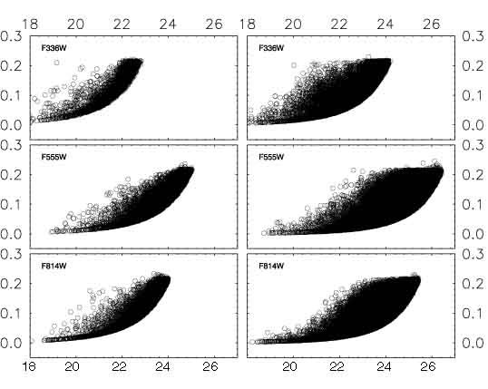
Figure 3: Residuals in magnitudes for the WFPC2 filters F336W, F555W, and F814W. The results in the left column correspond to the lists from proposal 6716. The plots in the right column are those from proposal 6569.

We analyzed the photometric errors as a function of magnitude for all the considered filters. The photometric uncertainties are determined for each star based upon statistical errors, sky determination errors and aperture correction errors. We found that some points clearly exceed the statistical errors, especially in the F555W and F814W bands: these are stars deeply embedded in the H II regions where line emission significantly enhances the local background. Figure 3 presents six plots of the magnitude errors as a function of magnitudes F336W, F555W, and F814W obtained using our photometry lists from proposals 6716 and 6569.

2.2 STIS Observations and reduction

We summarize the STIS data sets analyzed for this study in Table 1. All the UV observations employed the STIS near–ultraviolet (NUV) Cs₂Te Multi-Anode Microchannel Array (MAMA) detector. This detector has a field of view of $25"\times 25"$ and a pixel size of $\approx 0\farcs 02468.$ The images were obtained from proposal 9096 (P.I.: Jesús Maíz-Apellániz) and they show the two targets, regions NGC4214–I and NGC4214–II, with higher resolution than the WFPC2 images.

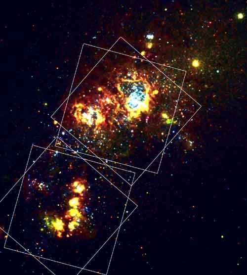
Figure 4: HST/STIS fields drawn over a WFPC2 color mosaic of NGC 4214. Each field corresponds to one visit. The mosaic was built using original images in filters F336W (blue), F555W+[O III] $\lambda$5007 (green), and F814W+H$\alpha$ (red). The field shown is the same as in Figure 2.

Each target was imaged using two different orientations shown in Figure 4. This is an RGB mosaic which we made by assigning the F336W image to the blue pixel values, the F555W+[O III] $\lambda$5007  images to the green pixel values, and the F814W+H$\alpha$  images to the red pixel values. Filter F25CN182 (F25CN270) provides medium–band width imaging with a central wavelength of 1820 Å (2700 Å) and an FWHM of 350 Å (350 Å). The STIS data were reduced by the STScI calibration pipeline, via the on–the–fly reprocessing which uses the best calibration reference files available at the time of retrieval from the HST archive. This used the latest geometric distortion correction taken from Maíz-Apellániz & Úbeda (2004).

Comparing Figures 1 and 4 we see that the STIS field–of–view is situated within the WFPC2 images of NGC 4214. We obtained the coordinates of all objects in our 11 STIS images using a customized version of the DAOFIND task in the DAOPHOT software package Stetson (1987) running under IDL and then we performed aperture photometry on all the images. We cross–correlated the 11 STIS photometric lists with the list obtained from the WFPC2 images using F336W as reference filter (LIST336). We found that a few stars in the WFPC2 list have two or more counterparts in the STIS list. This is the result of the fact that STIS has a higher resolution than WFPC2. At the distance of NGC 4214 (2.94 Mpc), the problem of multiple unresolved systems is unavoidable. For example: Maíz-Apellániz et al. (2005) study the problem derived from stellar multiplicity in the determination of initial mass functions. They present results for Trumpler 14, a massive young cluster in the Carina Nebula that contains at least three very–early O–type stars. If this cluster were located at a distance similar to that of NGC 4214, it would appear as a point source even though we know for certain that it is a multiple system. We use this result to justify our approach to solve this issue, by including a combination of objects as a single object in our final list.

2.3 Completeness tests

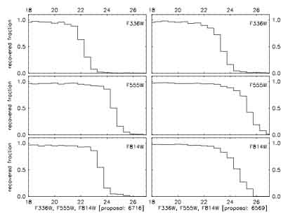
Figure 5: Completeness levels of the WFPC2 photometry based on artificial star tests performed using HSTphot (Dolphin, 2000). The fraction of recovered artificial stars is plotted against the magnitude for filters F336W, F555W, and F814W. The results in the left column correspond to the tests performed on images from proposal 6716. The plots in the right column are the tests performed on images from proposal 6569.

The detailed analysis of NGC 4214 data (such as the study of the B/R ratio and the derivation of an IMF) require a quantitative evaluation of completeness of the photometric data. We therefore conducted several experiments in which we added artificial stars with known magnitude and position to the images and then attempted to recover them using the same finding procedures that we used for the real stars. This was done using routines within the HSTphot suite of codes. The artificial stars were given random magnitudes and colors in the range $14\leq$F336W $\leq 26$ and $-2.0\leq$ F336W – F555W $\leq 4.0$. Approximately 50 000 fake stars were added in each image in all four chips. HSTphot generates a grid of artificial stars which are distributed according to the flux of the image, so that crowded areas would contain more fake stars than less crowded ones. Then the artificial stars were detected and measured using the same algorithms that we used for the observed data. To be recovered, a star must have survived the fitting process, having been found automatically and it must have passed the cross–identification test. The ratios of recovered to inserted stars in the different magnitude bins give directly the completeness factor as a function of magnitude. In Figure 5, we plotted the results of the artificial star tests for filters F336W, F555W, and F814W in proposals 6569 and 6717 and we observe that, at the bright end, the completeness is about 95% or higher in all images. For fainter magnitudes, the completeness falls off more quickly with increasing magnitude in the images obtained in proposal 6716 than in those obtained in proposal 6569, as expected from the shorter exposure times of the former.

The next step was to map the Hertzsprung–Russell diagram as a finely spaced grid, and to calculate the completeness values at each point. In order to do this, we used CHORIZOS (see Section 2.5) to obtain two useful relationships: the relation between F336W – F555W and $T_{\mathrm{eff}}$; and the relation between F336W – F555W and $M_{\mathrm{bol}}$ for $E(4405-5495)=0.1$ mag which is a typical value of the extinction in NGC 4214 as estimated by Leitherer et al. (1996). This procedure was only used to estimate the completeness values which we list on Table 4, not to determine stellar or cluster physical properties. A separate independent study of completeness for the STIS data was not necessary, because we matched all the stars in the STIS lists to stars in LIST336. Therefore, the completeness tests conducted for LIST336 include both WFPC2 and STIS data. Since the STIS images go deeper than the WFPC2 data, our results are limited by the depth of the WFPC2 images.

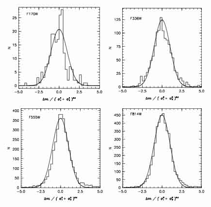
Figure 6: Histograms for the measured magnitude difference normalized by the experimental uncertainty ( $\Delta m/\sqrt{\sigma_{1}^{2}+\sigma_{2}^{2}}$ ). Here we are comparing magnitudes of stars observed in two different visits during proposal 6716. See text for details about the method. The black curve shows the expected normal distribution.

In order to check for the consistency of our data, we used the fact that NGC 4214 was visited twice for proposal 6716: first on June 29, 1997 and later on December 09, 1997. The orientation of the cameras in the sky was different for both visits as can be clearly seen in Figure 1. It is important to note that the idea behind this proposal was to obtain the best resolution of regions NGC 4214–I and NGC 4214–II and that is why those complexes are centered in the PC. The fields of view that correspond to both visits in proposal 6716 contain a significant amount of overlap, allowing us to test the internal consistency of the photometry in order to check for possible systematic uncertainties introduced by the CTE or contamination corrections. For each of the four filters in this proposal we obtained two photometric lists, one for each visit to NGC 4214. We then performed a statistical test on all the objects which were identified as the same star in the two lists. We calculated the distribution of $(m_{1}-m_{2})/\sqrt{\sigma_{1}^{2}+\sigma_{2}^{2}}$, where $m_{i}$ and $\sigma_{i}$ are the magnitude and its uncertainty in list $i$. This distribution closely resembles a normal distribution with zero mean and a standard deviation of unity for all the filters used, as we show in the histograms in Figure 6. The total number of points (N) considered for the histograms, the average value of $\Delta m/\sqrt{\sigma_{1}^{2}+\sigma_{2}^{2}}$ and its standard deviation are given in Table 5. The same study with filters F25CN182 and F25CN270 was performed for our STIS lists. Again, we obtained histograms that closely resemble a normal distribution with zero mean and standard deviation of unity, showing the agreement between different photometric lists.

The completeness values obtained in this section will allow us to better estimate the actual number of blue and red supergiants in the galaxy. We will also use them to infer the initial mass function as we explain in detail in Paper II.

2.4 Cluster photometry

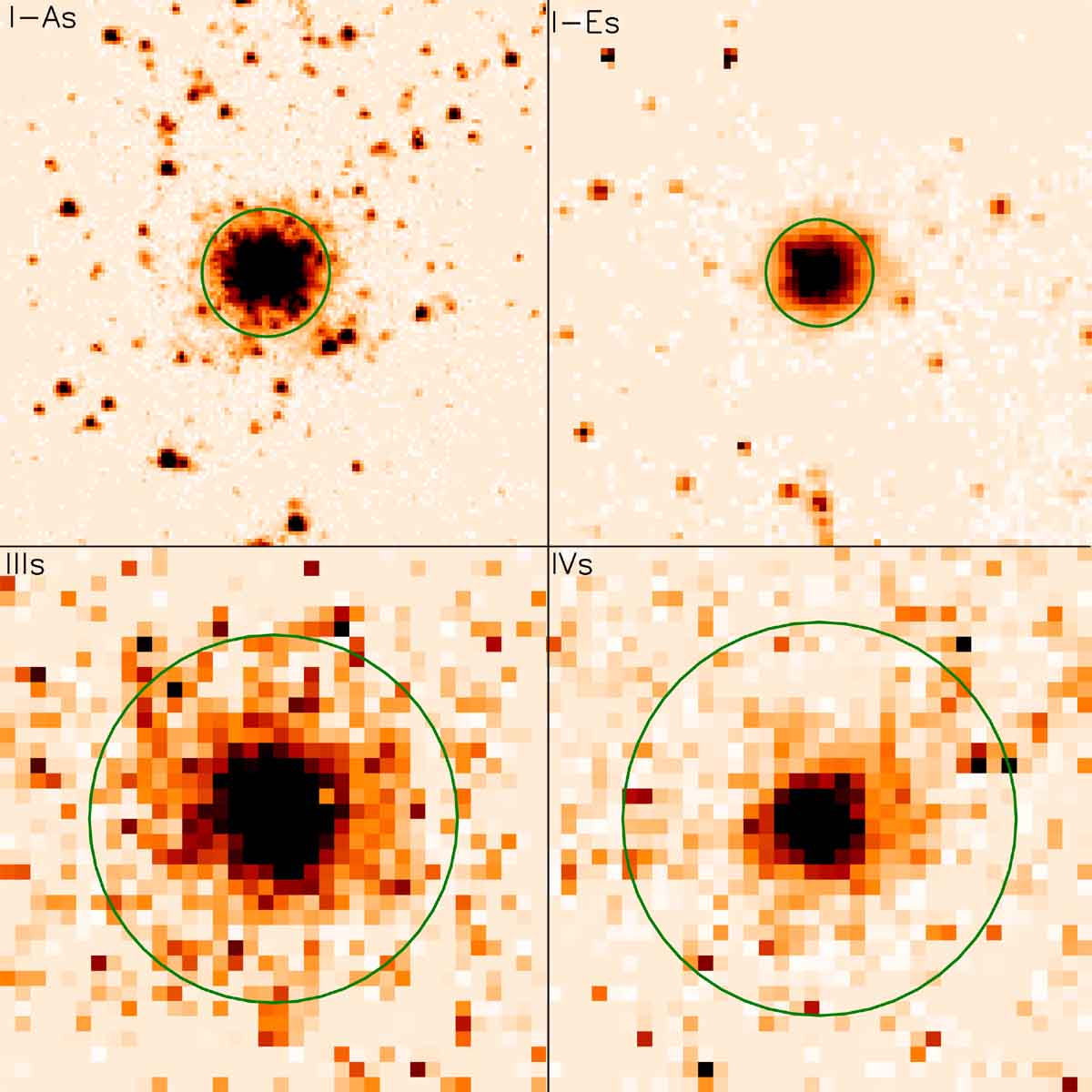
Figure 7: HST images of star clusters I–As, I–Es, IIIs, and IVs. The images have been scaled in order to use the same linear size, with the field being $50$ pc $\times 50$ pc in all cases. North is up and east is left. The circles depict the apertures used for our photometry. Cluster I–As is shown on a STIS image in filter F25CN270. We used a WFPC2/PC image in filter F555W to show cluster I–Es. Clusters IIIs and IVs are depicted on WFPC2/WF F814W images. These images clearly show the different pixel size (and resolution) of the three cameras that we have used.

The HSTphot package (Dolphin, 2000) was developed specifically to obtain stellar photometry of point sources on images obtained with HST WFPC2. Our WFPC2 and STIS images contain some objects (I–As, I–Es, IIIs, and IVs) which are known to be unresolved stellar clusters, and which appear as extended sources rather than point–like objects. The position of these clusters is shown in Figure 2, and their corresponding blowups are in Figure 7. Other clusters are resolved into stars and we also analyzed them using aperture photometry. These clusters are organized in two groups: large complexes (which include smaller clusters): I–A, I–B, and II; and resolved clusters: I–Ds, II–A, II–B, II–C, II–D, and II–E. Their positions in the galaxy are shown in Figure 2.

We performed detailed aperture photometry of these clusters, carefully selecting the aperture radii and the sky apertures. We used the closest possible radii values to those provided by (MacKenty et al., 2000). In all cases we included more than 90% of the light from each cluster, with the exception of cluster I–As, which presents an extended halo. See Paper II for a full discussion. We used custom made IDL codes to perform this task on WFPC2 and STIS CCD images. The values of the aperture correction (in magnitudes) that we used to calculate the aperture correction for the STIS images are taken from Proffitt et al. (2003) which refer to point sources. When the cluster was bright enough and no confusion with nearby sources was apparent, we measured the $JHK_{s}$ photometry from 2MASS data using the same apertures that we had used with the WFPC2 and STIS images. Clusters IIIs and IVs have their $JHK_{s}$ magnitudes listed in the 2MASS catalogue. We compared the profile fitting and the aperture photometric measurement provided by 2MASS with our own measurements to determine an aperture correction. This correction was required to compare the 2MASS magnitudes with the WFPC2 ones, given the different spatial resolutions. The complete photometry of all the clusters is summarized in Tables 6 and 7.

2.4.1 Unresolved clusters

Images from proposal 6716 show cluster I–As on the PC of the WFPC2, while those of proposal 6569 picture this region on the WF3. This cluster is the brightest feature in NGC 4214 at optical wavelengths, and its pixels appear saturated in some images (filter F555W in proposal 6716; filters F336W, F555W, and F702W in proposal 6569.) This object can also be seen in some of our STIS images. Unfortunately, images obtained during programme 6716 on December 1997 show a bad column passing through cluster I–As; in order to get rid of this problem, we interpolated the number of counts in each pixel along the column using the pixels from two adjacent columns of the chip. Aperture photometry was obtained using an aperture radius of 9 PC pixels which is equivalent to $5.84$ pc at a distance of 2.94 Mpc, or $0\farcs 41.$ The adopted equatorial coordinates of the cluster are given in Table 8. Once we obtained the magnitudes in all the available images, we calculated a weighted mean for each filter, using their own errors as weights.

A small cluster can be seen between I–A and I–B: cluster I–Es. It was imaged in proposal 6716 images using filters F170W, F336W, F555W, and F814W on the PC. It was also captured in all the images from proposal 6569 on the WF3 camera. This object can also be seen in some of our STIS images. Some images of this cluster show a bad column and we solved this problem using the same technique as we did for cluster I–As.

Cluster IIIs can be found in proposal 6716 images in filters F170W, F336W and F814W on the WF4. It appears as a saturated object in filter F555W. It was also found in all the images from proposal 6569 on the WF3 camera, but the central pixels are saturated in image F702W. On images from proposal 6716, the cluster appears very near the vignetted field between the PC and the WF4. For this reason, we thought that the calculated magnitudes might be affected and we discarded all of them except for the magnitude obtained with filter F170W, and we relied on the magnitudes obtained with images from proposal 6569. Aperture photometry was obtained using an aperture radius of 12 WF pixels which is equivalent to $17.1$ pc at a distance of 2.94 Mpc. Once we obtained the magnitudes in all the available images, we calculated a weighted mean for each filter. This object is present in the 2MASS All–Sky Catalog of Point Sources (Skrutskie et al., 2006) and is located in a relatively isolated region, which provided us with useful magnitudes in the $J$, $H$ and $K_{s}$ bands. Nevertheless, an aperture correction was required in order to compare those magnitudes with the WFPC2 ones, given the different spatial resolutions. The field–of–view of the available NICMOS images does not cover the clusters analyzed in this paper.

Cluster IVs falls on the vignetted field between the WF3 and the WF4 on the proposal 6716 images, making it impossible to calculate its magnitude in those images. This object is clearly visible in proposal 6569 images in filters F336W, F555W, F702W and F814W pictured on the WF3. Aperture photometry was obtained using an aperture radius of 11.40 pc or $0\farcs 8.$ Cluster IVs is also listed in the 2MASS Catalog. We retrieved its $J$, $H$ and $K_{s}$ magnitudes and corrected them for aperture effects as we did for cluster IIIs. The complete photometry of these clusters is summarized in Table 6.

2.4.2 Large complexes of smaller clusters or SOBAs

We performed aperture photometry for complexes I–A, I–B, and II using aperture radii very similar to the ones that that MacKenty et al. (2000) use to describe the clusters. We centered cluster I–A at a position slightly displaced from cluster I–As. Whenever we found bad columns in our images, we corrected them using the same procedure that we employed for cluster I–As. Some of our images have some saturated pixels within an aperture radius of 150 PC pixels; those filters were discarded. We were able to obtain the photometry of this cluster in images with filters F170W, F336W, F814W, F25CN182, and F25CN270.

Another cluster which is part of the large complex NGC 4214–I is cluster I–B, which is located to the south–east of cluster I–A. We used an aperture radius of 42.18 pc ($2\farcs 96$). We were not able to use the images from proposal 6569 because this cluster lies very close to the vignetted section of the chips. Some of the images in proposal 6716 have bad columns across the cluster.

The other large nebular structure in the galaxy is NGC 4214–II. This complex part of NGC 4214 is very well imaged on the WF4 chip from proposal 6716, on the WF2 chip from proposal 6569, and on some of our STIS images. We used an aperture radius of 200 PC (or 91 WF) pixels to perform the photometry. We encountered some bad columns extending across this cluster, specially through clusters II–A, and II–C.

Using the images provided by the 2MASS All–Sky Survey, we performed aperture photometry in filters $J$, $H$, and $K_{s}$ for clusters I–A, I–B, and II. We used the centers and aperture radii given in Table 8. To calibrate our measurements, we used the magnitudes given by the 2MASS All–Sky Catalog for clusters IIIs and IVs, which were calculated using a $4\farcs 0$ aperture radius. Since the sky in these images is very noisy (the number of counts in the sky is of the order of counts in the clusters), we obtained big errors in our 2MASS photometry. The complete photometry of these clusters is summarized in Table 6.

2.4.3 Resolved clusters

Cluster I–Ds is composed of a small group of stars located towards the north of cluster I–A, and has only a small amount of gas in its surroundings (MacKenty et al., 2000). A small aperture of 20 PC pixels (12.97 pc) was used for the photometry. This cluster falls out of the field–of–view of our STIS images. It is located near the vignetted area in the WF3 camera chip from proposal 6569. We also found it on the PC in one of the visits from proposal 6716 and on the WF4 in the other visit.

We performed a detailed analysis of the structure of cluster II by examining its five components (II–A, II–B, II–C, II–D, and II–E.) These fairly well–resolved clusters are embedded within several H$\alpha$ regions as can be observed comparing Figures 2 and  4. To perform the aperture photometry, we followed the same routine as for cluster II, taking into account the bad columns in all cases. The aperture radii for these clusters are 50, 37, 57, 32, and 35 PC pixels respectively or 32.49, 23.94, 36.91, 20.81, 22.66 pc respectively. The complete photometry of these clusters is summarized in Table 7.

2.5 SED fits using CHORIZOS

Our images provide photometric magnitudes in various filters, which represent the main observable. To translate these observables into fundamental stellar/cluster parameters – e.g. effective temperature ($T_{\mathrm{eff}}$), bolometric magnitude ($M_{\mathrm{bol}}$), and cluster age – we used CHORIZOS (Maíz-Apellániz, 2004), an IDL package that fits an arbitrary family of spectral energy distribution models (SEDs) to multi–color photometric data. The fundamental parameters are determined simultaneously by a likelihood–maximization technique from the photometric colors calculated from the measured magnitudes. The associated errors for these parameters are computed from the resulting likelihood multidimensional array. We applied CHORIZOS to stars and clusters separately, using different sets of theoretical models.

2.5.1 Application to stars

We applied CHORIZOS to our observed stellar magnitudes to measure the effective temperature, monochromatic color excess [ $E(4405-5495)$, see e.g. Maíz-Apellániz 2004 for its relationship to $E(B-V)$ ], and (when possible) extinction law of the stars in our sample. For the stars we used as input SEDs low–gravity Kurucz models with $\log(Z/Z_{\sun})=-0.5$. The stars in LIST336 were treated in the following way:

six and five filters

All the stars with six and five observed magnitudes were processed through CHORIZOS first. For these objects $T_{\mathrm{eff}}$, $E(4405-5495)$, and the extinction law were left as free parameters. The extinction law was chosen among the $R_{5495}$–dependent family of Cardelli et al. (1989), and the MC laws of Misselt et al. (1999) and Gordon & Clayton (1998).

four filters

For the objects with only four observed magnitudes (three independent colors), the extinction law was restricted to three values in three different runs: First we ran the code using an SMC–like extinction law; as a second experiment, we used a Galactic–extinction law with the widely used value $R_{5495}=3.1$, and for the last experiment we fixed the value $R_{5495}=5.0$. We compared the values of the goodness of the fit $(\chi^{2})$ for each star and kept the results that correspond to the lowest value of $\chi^{2}.$ For this set of objects we had three independent colors and, having fixed the extinction law, only two parameters to be determined: $T_{\mathrm{eff}}$ and $E(4405-5495)$.

three filters

The remaining objects with only three observed magnitudes were processed through CHORIZOS leaving only $T_{\mathrm{eff}}$ and $E(4405-5495)$ as free parameters and using the extinction law of Cardelli et al. (1989), with $R_{5495}=3.1$. For this set of objects, we had only two independent colors and we had to fix at least one parameter. This left us with zero degrees of freedom but this is the best that can be done with only three observed magnitudes.

It is well known from studies of our own and other galaxies that the extinction law can vary in small (less than 1 pc) spatial scales (see Arias et al. (2006) for a recent study). We decided to fix $R_{5495}=3.1$ to the objects with three and four filters, because this value is very close to the mean values of $R_{5495}$ calculated for stars with five and six filters, where we left $R_{5495}$ as a free parameter in the fit, and because $R_{5495}=3.1$ is the standard value measured in the Galaxy.

Objects in LIST814 have magnitudes in three WFPC2 filters: F555W, F702W, and F814W, with which we built two photometric colors: F555W–F702W and F555W–F814W. In this case, the maximum allowed number of free parameters is two but, for this specific filter combination, there are strong color degeneracies that hamper the simultaneous determination of $T_{\mathrm{eff}}$ and $E(4405-5495)$. Therefore, we decide to use our extinction results (see Paper II) by restricting $E(4405-5495)$ to the range $-0.05\leqslant E(4405-5495)\leqslant 0.25$ and by fixing $R_{5495}=3.1$, as explained above.

In order to assess the goodness of the fit we rely on the value of $\chi^{2}$ provided by CHORIZOS for each star. All objects with $\chi^{2}\leq 4.0$ were considered as good fits throughout our work. We performed a detailed analysis of those objects from lists with six and five filters with $\chi^{2}>4.0$. An inspection of the output plots which shows the theoretical spectrum overplotted on the measured magnitudes, reveals in some of these cases that one or two of the observed magnitudes are not in agreement with the rest. This may be due to several reasons, such as strong nebular contamination in F555W or unresolved multiple systems. Those cases were analyzed on a one–to–one basis. In all these cases, we accordingly removed one or two magnitudes from the list (e.g. F555W for a star with strong nebular contamination or F814W for an early–type star with an apparent late–type companion) and reran CHORIZOS with the new set of magnitudes.

The output of CHORIZOS  that corresponds to the stellar components of NGC 4214 will be used to analyze various aspects of this galaxy: In this paper we present two Hertzsprung–Russell diagrams from which we infer the galaxy’s stellar population. In Paper II we will implement these results to study the variable extinction throughout our field–of–view, to calculate the blue to red supergiant ratio, and to determine the initial mass function slope using the most direct and reliable method which is based on counts of stars as a function of their luminosity/mass.

2.5.2 Application to clusters

The extended sources in our sample (both resolved and unresolved) were treated in a different way. CHORIZOS includes precalculated Starburst99 (Leitherer et al., 1999) cluster models, where the intrinsic parameters are the cluster age and its metallicity and the external parameters are the same as in the stellar case: $E(4405-5495)$ and $R_{5495}$. These models are tabulated for a Salpeter (1955) stellar initial mass function of 1 to 100 $M_{\sun}$. The exact low mass limit of the IMF is not important for our age determinations because the integrated colors of clusters with ages younger than $10^{8}$ years are dominated by stars with masses greater than 1 $M_{\sun}$, but it is relevant for the determination of the total mass.

For all our clusters we used Starburst99 models of integrated stellar populations with metallicity $Z/Z_{\sun}=0.4$, appropiate for NGC 4214 (Kobulnicky & Skillman, 1996), and ages of the models varying between $\log({\rm age/yr})=6.0$ and $\log({\rm age/yr})=9$. The available reddening values $E(4405-5495)$ are in the range $0.0-5.0.$ For the extinction law, we considered the $R_{5495}-$dependent family of Cardelli et al. (1989) (Galactic extinction); the average LMC and LMC2 laws of Misselt et al. (1999) (extinction of the LMC), and the SMC law of Gordon & Clayton (1998) (extinction of the SMC).

The comprehensive study of the CHORIZOS output is presented in Paper II, where we address several issues such as the determination of clusters age, mass, and massive stellar constituents. We analyze the different solutions for each cluster and we present arguments to choose the best possible model that fits our data in each case. In Paper II, we will also discuss the problems that arise when using large and small aperture radii.

3 General description of the observed stellar populations

With the output values of CHORIZOS from the stellar analysis, we can build a theoretical Hertzsprung–Russell diagram for NGC 4214. These diagrams allow us to compare our observations with stellar evolution models and to interpret them in physical terms such as mass, age, composition etc. We used sets of evolutionary tracks provided by Lejeune & Schaerer (2001). These use the entire set of non–rotating Geneva stellar evolution models covering masses from $0.8$ to $120M_{\sun}$.

NGC 4214 is moderately metal deficient, with an abundance of $12+\log(\mathrm{O/H})=8.15-8.28$ (Kobulnicky & Skillman, 1996) or about $Z=0.34Z_{\odot}=0.006$ using the results provided by Massey (2003) for the MCs and the Galaxy. We bracketed the data between theoretical models with metallicities $Z=0.004$ and $Z=0.008$, which are the closest available to the estimated metallicity of NGC 4214 $(Z\approx 0.006).$

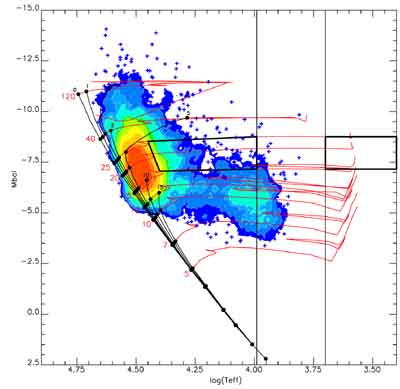
Figure 9: Hess diagram for all stars in LIST336 (the main photometric list using F336W as reference filter) with calculated $M_{\mathrm{bol}}$and $T_{\mathrm{eff}}$ obatined from the CHORIZOS output. The contour levels correspond to stellar counts of 5, 10,15,20,40,50,75,100,150, and 200 objects per element. Each element measures 0.0875 mag in the $M_{\mathrm{bol}}$ axis and 0.0075 in the $\log(T_{\mathrm{eff}})$ axis. Individual stars are shown as small crosses in those regions of the diagrams where the density was lower than 5 stars. The red lines represent the evolutionary tracks for stars in the mass–range 5, 7, 10, 12, 15, 20, 25, 40, and 120 $M_{\sun}$. The solid black lines represent the isochrones calculated for ages 0, 1, 2, 3, 5, 10, and 15 Ma. This diagram also shows two polygons between tracks labeled 15 and 25 $M_{\sun}$. These are the regions that we will use to count blue and red supergiants in Paper II.

These theoretical models provide the luminosity, age, and effective temperature of representative evolutionary points. We calculated seven isochrones by interpolating the bolometric magnitudes as a function of the logarithm of the age along each mass track in steps of $1-5$ million years (ZAMS, 1Myr, 2Myr, 3Myr, 5Myr, 10Myr, and 15Myr.) The Hertzsprung–Russell diagrams of NGC 4214 are presented in Figures 8 and 9.

We have separated the stars in two diagrams: Figure 8 is a plot of objects from LIST814 and Figure 9 is a plot of objects taken from LIST336. Instead of representing individual stars, we display contour plots to show the varying density of stars in the [ $\log(T_{\mathrm{eff}})$, $M_{\mathrm{bol}}$ ] plane also referred to as Hess diagrams. The contour levels correspond to stellar counts of 10, 15, 20, 40, 50, 100, 300, 600, 1200, and 2000 objects per HRD element in Figure 8, and 5, 10, 15, 20, 40, 50, 75, 100, 150, and 200 objects per HRD element in Figure 9. Each HRD element measures 0.0875 mag in the $M_{\mathrm{bol}}$ axis and 0.0075 in the $\log(T_{\mathrm{eff}})$ axis. Individual stars are shown as small crosses in those regions of the diagrams where the density was lower than 10 and 5 stars respectively .

As a dwarf irregular galaxy, NGC 4214 is an interesting laboratory where the process of star formation can be studied. This is a young galaxy which is still processing gas into stars. It is a relatively gas–rich system with a young stellar population of bright, blue stars and H II regions. The star formation regions are concentrated along a bar structure surrounded by a large disk of gas. A second, less intense, region of recent star formation, is located off the northern tip of the bar at a distance of about 2 kpc from the galactic center but is not covered by the HST data (see Figure 1). Because the ISM is readily ionized by the intense UV radiation from young stars in H II regions, H$\alpha$ is often used as an indicator of the presence of recent star formation. Figure 4 pictures the regions of star formation through the H$\alpha$ tracer.

Figures 8 and 9 allow us to analyze the stellar population of NGC 4214. Figure 8 shows the objects from LIST814. The most striking feature present in this plot is the crowded clump in the red part of the diagram. This feature shows a great concentration of stars in the range $3.50\leqslant\log(T_{\mathrm{eff}})\leqslant 3.75$. It is composed of the red giant locus, the asymptotic giant branch, and, along its blue extent, of intermediate age blue loop stars. Most probably, these stars represent a mixed–age population that has evolved off the zero–age main sequence. A group of red supergiants stars can be seen at the tip of the red plume. These are stars with initial masses $\gtrsim 40M_{\odot}$ which had evolved past the main sequence and into the RSG phase. One noticeable fact is that some of the stars are located to the right of the extreme of the evolutionary tracks. This fact has been observed by Massey & Olsen (2003) while studying RSGs in the Magellanic Clouds. The evolutionary tracks do not go far enough to the right (cool temperatures) to produce the RSGs that are actually observed. The same problem was mentioned by Massey (2003) for Galactic RSGs. Levesque et al. (2005) present a new effective temperature scale for Galactic RSGs by fitting MARCS stellar atmosphere models (Gustafsson et al., 1975; Plez et al., 1992) which include an improved treatment of molecular opacity to 74 Galactic $(Z=0.020)$ RSGs of known distance. Their main result is that RSGs appear to be warmer than previously thought. This effect shifts the stars to the left in the diagrams (by $\sim 300-400$ K) making them coincide with the end of the tracks.

Figure 9 is characterized by a blue plume of stars. This is the realm of the H–burning (main–sequence) massive stars. The locus of these stars lies above the $5M_{\odot}$ evolutionary track and extends up to $M_{\mathrm{bol}}\approx-14.$ It is well populated in the range $\approx 12M_{\odot}-60M_{\odot}$, indicating some ongoing star formation. In the figure we can clearly see a group of objects lying along the main sequence, indicating that these are young objects. However, for large masses, the mean locus of the position of the stars is located to the right (lower temperatures) of this sequence. This is likely to be caused by a combination of two effects: the difficulty of observing ZAMS stars at high mass (because they are in highly extinguished regions) and the existence of unresolved stellar systems (which also has the consequence of producing a number of points above the $120M_{\odot}$ track). The other feature in this diagram is the group of stars located between the $5M_{\odot}$ and the $20M_{\odot}$ evolutionary tracks, and with $\log(T_{\mathrm{eff}})\lesssim 4.25$. These objects are evolved massive stars with ages greater than 15 Myr.

We agree with Drozdovsky et al. (2002) in that stars appear to populate the Hertzsprung–Russell diagram  of NGC 4214 throughout all of the major phases of stellar evolution, leading one to conclude that the star formation was more or less continuous in recent times, although there could have been some recent starbursts present. Most of the brightest stars in the galaxy are concentrated towards the two main regions of star formation, which are NGC 4214–I and NGC 4214–II. These are regions characterized by different morphology, which MacKenty et al. (2000) interpret as an evolutionary or aging trend. The stellar components of NGC 4214-II are co-spatial with the gas, and individual massive stars can be seen in different stages of stellar evolution. As we show in Paper II, this is the youngest (age $\approx$ 2 Myr) region in the galaxy. On the other hand, NGC 4214–I (age $\approx 3-5$ Myr) shows some signs of cluster evolution, with evacuated cavities produced by winds and supernova explosions. Younger stars tend to concentrate around the main two clusters (I–A and I–B) in this part of the galaxy. Concentrations of bight stars are also detected outside the central area, outlining a bar structure which is a characteristic of NGC 4214. The crowded clump in the red part of the diagram in Figure 8 suggests that the galaxy possesses a significant underlying intermediate–age / old population. This fact is reinforced by the prominent red halo observed in Figure 1. The analysis of Maíz-Apellániz et al. (1998) shows that the older population contributes to around 50 % of the optical continuum. This population does not contribute to the UV continuum, but dominates the emission in the IR. All this means that the present burst is not the first episode of star formation in the nucleus of NGC 4214.

4 Summary and conclusions

In this paper we present the HST/WFPC2 and HST/STIS observations of the well–resolved nearby galaxy NGC 4214. We obtained PSF photometry of the stellar components and aperture photometry of some interesting clusters using high resolution images. We explain how we managed to translate observed quantities such as magnitudes and photometric colors into physical parameters such as $T_{\mathrm{eff}}$, and $M_{\mathrm{bol}}$ for stars, and age for clusters, using CHORIZOS (Maíz-Apellániz, 2004).

The stellar content of NGC 4214 has been discussed using two [ $\log(T_{\mathrm{eff}})$, $M_{\mathrm{bol}}$ ] Hertzsprung–Russell diagrams: one shows the stars from a list with filter F336W as reference, and the other was built with filter F814W as reference. The first diagram shows most objects on the main–sequence, while the second diagram is characterized by a crowded concentration of stars in the range $3.50\leqslant\log(T_{\mathrm{eff}})\leqslant 3.75$.

In Paper II we will present the following results: the blue to red supergiant ratio, an estimate of the initial mass function, a study of the variable extinction throughout the galaxy, and a detailed analysis of the cluster population.

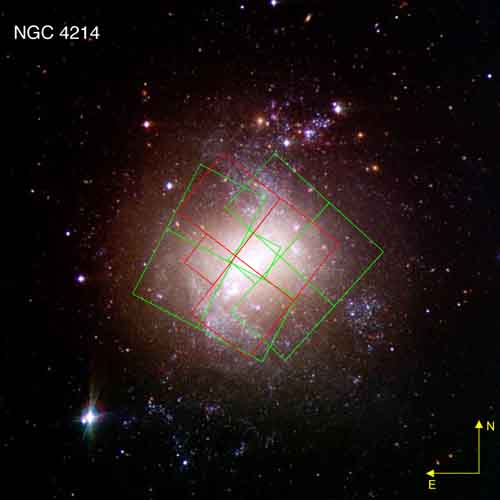
Figure 1: $9\arcmin\times 9\arcmin$ (7.7 kpc $\times$ 7.7 kpc) image of NGC 4214 from an RGB combination of public B, V and R band images obtained with the Isaac Newton Telescope. HST/WFPC2 fields (green) are overplotted for proposal 6716. The left field corresponds to the second visit (09 Dec 1997) and the right field corresponds to the first visit (29 Jun 1997). The HST/WFPC2 field from proposal 6569 is displayed in red (center field).

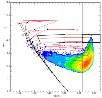
Figure 8: Hess diagram for all stars in LIST814 (the main photometric list using F814W as reference filter) with calculated $M_{\mathrm{bol}}$and $T_{\mathrm{eff}}$ obtained from the CHORIZOS output. The contour levels correspond to stellar counts of 10, 15, 20, 40, 50, 100, 300, 600, 1200, and 2000 objects per element. Each element measures 0.0875 mag in the $M_{\mathrm{bol}}$ axis and 0.0075 in the $\log(T_{\mathrm{eff}})$ axis. Individual stars are shown as small crosses in those regions of the diagrams where the density was lower than 10 stars. The red lines represent the evolutionary tracks for stars in the mass–range 5, 7, 10, 12, 15, 20, 25, 40, and 120 $M_{\sun}$. The solid black lines represent the isochrones calculated for ages 0, 1, 2, 3, 5, 10, and 15 Ma. This diagram also shows two polygons between tracks labeled 15 and 25 $M_{\sun}$. These are the regions that we will use to count blue and red supergiants in Paper II.

Table 1: Journal of observations, with filters and exposure times for WFPC2 and STIS images. The dates of the observations are given in the main text.

Proposal	Filter	Band	Dataset	Exposure Time (s)
	F336W	WFPC2 U	u3n80101m + 2m + 3m	260 + 900 + 900
	F555W	WFPC2 V	u3n80104m + 5m + 6m	100 + 600 + 600
6569	F702W	WFPC2 wide R	u3n80107m + 8m	500 + 500
	F814W	WFPC2 I	u3n8010am + bm + cm	100 + 600 + 600
	F170W	UV	u4190101r + 102r + 201m + 202m	400 + 400 + 400 + 400
	F336W	WFPC2 U	u4190103r + 104r + 203m + 204m	260 + 260 + 260 + 260
6716	F555W	WFPC2 V	u4190105r + 205m	200 + 200
	F814W	WFPC2 I	u4190106r + 206m	200 + 200
	F25CN182		o6bz02isq + 02iwq + 01afq	288 + 288 + 288
	F25CN182		o6bz04r8q + 04raq + 03afq	288 + 288 + 288
9096	F25CN270		o6bz02j7q + 02jbq + 03awq	288 + 288 + 288
	F25CN270		o6bz04ruq + 04ryq	288 + 288

Table 2: Photometry of stars in LIST336. The photometric uncertainties are determined for each star based upon statistical errors, sky determination errors and aperture correction errors. The complete lists is in the electronic version of this paper.

$\alpha$ (J2000)	$\delta$ (J2000)	F336W	F170W	F555W	F702W	F814W	CN182	CN270
12:15:37.802	36:19:44.200	$17.55\pm 0.01$		$19.06\pm 0.01$	$18.90\pm 0.01$	$18.94\pm 0.04$
12:15:39.584	36:19:35.376	$17.66\pm 0.04$	$17.67\pm 0.10$	$19.08\pm 0.07$		$19.03\pm 0.04$	$17.43\pm 0.12$	$17.22\pm 0.11$
12:15:40.561	36:19:33.604	$17.86\pm 0.02$	$18.00\pm 0.10$	$19.24\pm 0.01$		$19.16\pm 0.02$	$18.04\pm 0.14$	$17.73\pm 0.12$
12:15:39.586	36:19:29.245	$17.87\pm 0.01$	$17.25\pm 0.06$	$19.57\pm 0.05$	$19.57\pm 0.05$		$17.04\pm 0.11$	$17.18\pm 0.11$
12:15:40.574	36:19:33.422	$17.88\pm 0.06$	$16.78\pm 0.08$	$19.62\pm 0.07$		$19.74\pm 0.06$	$17.28\pm 0.12$	$17.65\pm 0.11$

Table 3: Photometry of stars in LIST814. The photometric uncertainties are determined for each star based upon statistical errors, sky determination errors and aperture correction errors. The complete lists is in the electronic version of this paper.

$\alpha$ (J2000)	$\delta$ (J2000)	F814W	F555W	F702W
12:15:41.449	36:18:59.382	$18.80\pm 0.00$	$20.79\pm 0.01$	$19.42\pm 0.00$
12:15:39.384	36:18:59.959	$18.83\pm 0.00$	$21.16\pm 0.01$	$19.59\pm 0.01$
12:15:33.382	36:19:25.804	$18.94\pm 0.00$	$25.32\pm 0.16$	$24.81\pm 0.22$
12:15:32.202	36:19:36.543	$18.95\pm 0.01$	$20.90\pm 0.04$	$19.51\pm 0.08$
12:15:38.633	36:20:40.951	$19.06\pm 0.00$	$20.51\pm 0.00$	$19.18\pm 0.00$

Table 4: Completeness values for each track from Lejeune & Schaerer (2001) and their corresponding main sequence lifetime ($\tau_{MS}$).

Track ($M_{\odot}$)	7	10	12	15	20	25	40	60	85	120
Completeness	0.041	0.263	0.497	0.705	0.855	0.899	0.929	0.946	0.953	1.000
$\tau_{MS}$ (Myr)	46.50	23.98	17.84	12.95	9.12	7.17	4.82	3.71	3.48	3.01

Table 5: Analysis of the consistency of the photometry using two WFPC2 photometry lists from proposal 6716 (P.I.: Theodore Stecher).

	F170W	F336W	F555W	F814W
N	189	1114	3219	4116
average	-0.120	-0.013	0.119	0.049
$\sigma\tablenotemark{b}$	0.839	0.915	0.841	0.847

Table 6: Photometry of unresolved clusters and of large complexes

Filter	Cluster I–As	Cluster I–Es	Cluster IIIs	Cluster IVs	Cluster I–A	Cluster I–B	Cluster II
F170W	13.47 $\pm$ 0.07	18.82 $\pm$ 0.52	16.77 $\pm$ 0.15		11.81 $\pm$ 0.02	13.54 $\pm$ 0.03	12.45 $\pm$ 0.04
F25CN182	13.50 $\pm$ 0.02	19.27 $\pm$ 0.10			11.99 $\pm$ 0.02	13.60 $\pm$ 0.02	12.91 $\pm$ 0.02
F25CN270	14.00 $\pm$ 0.03	19.56 $\pm$ 0.11			12.51 $\pm$ 0.01	14.17 $\pm$ 0.02	13.20 $\pm$ 0.02
F336W	14.46 $\pm$ 0.04	19.30 $\pm$ 0.03	16.82 $\pm$ 0.05	17.17 $\pm$ 0.03	12.96 $\pm$ 0.01	14.62 $\pm$ 0.01	13.59 $\pm$ 0.01
F555W		18.98 $\pm$ 0.05	16.59 $\pm$ 0.03	17.30 $\pm$ 0.01		15.83 $\pm$ 0.23	14.37 $\pm$ 0.04
F702W		18.27 $\pm$ 0.04		16.97 $\pm$ 0.01			14.04 $\pm$ 0.08
F814W	15.98 $\pm$ 0.02	17.90 $\pm$ 0.03	15.67 $\pm$ 0.03	16.75 $\pm$ 0.02	13.93 $\pm$ 0.01	15.55 $\pm$ 0.01	14.24 $\pm$ 0.01
$J$			14.74 $\pm$ 0.10	15.93 $\pm$ 0.13	14.43 $\pm$ 0.50	15.69 $\pm$ 0.25	14.27 $\pm$ 0.63
$H$			14.30 $\pm$ 0.11	15.55 $\pm$ 0.19	14.31 $\pm$ 0.88	15.05 $\pm$ 0.27	13.65 $\pm$ 0.70
$K_{s}$			13.87 $\pm$ 0.10	15.39 $\pm$ 0.20	13.54 $\pm$ 0.66	15.27 $\pm$ 0.42	13.71 $\pm$ 1.02

Table 7: Photometry of resolved clusters

Filter	Cluster I–Ds	Cluster II–A	Cluster II–B	Cluster II–C	Cluster II–D	Cluster II–E
F170W	15.51 $\pm$ 0.03	15.54 $\pm$ 0.18	15.26 $\pm$ 0.05	14.23 $\pm$ 0.04	16.39 $\pm$ 0.16	15.97 $\pm$ 0.13
F25CN182		15.63 $\pm$ 0.06	15.50 $\pm$ 0.02	14.67 $\pm$ 0.02	16.66 $\pm$ 0.06	16.12 $\pm$ 0.04
F25CN270		15.66 $\pm$ 0.06	15.70 $\pm$ 0.02	15.07 $\pm$ 0.02	16.96 $\pm$ 0.07	16.33 $\pm$ 0.04
F336W	16.39 $\pm$ 0.01	15.87 $\pm$ 0.01	16.04 $\pm$ 0.01	15.52 $\pm$ 0.01	17.30 $\pm$ 0.02	16.67 $\pm$ 0.01
F555W	17.62 $\pm$ 0.02	16.46 $\pm$ 0.08	16.87 $\pm$ 0.03	16.76 $\pm$ 0.06	18.12 $\pm$ 0.12	17.75 $\pm$ 0.06
F702W	17.54 $\pm$ 0.04	16.09 $\pm$ 0.07	16.56 $\pm$ 0.06	16.50 $\pm$ 0.12	18.00 $\pm$ 0.22	17.48 $\pm$ 0.05
F814W	17.43 $\pm$ 0.03	16.46 $\pm$ 0.08	17.02 $\pm$ 0.01	16.72 $\pm$ 0.01	18.21 $\pm$ 0.01	17.93 $\pm$ 0.01

Table 8: The clusters astrometry and aperture radii.

Cluster	$\alpha$ (J2000)	$\delta$ (J2000)	Radius	Radius
	$12^{h}15^{m}+$	$36^{\circ}+$	[”]	[pc]
I–As	39.54	19 36.49	0.41	5.84
I–Es	40.26	19 39.94	0.36	5.13
IIIs	38.27	19 46.29	1.20	17.10
IVs	37.34	19 58.20	0.80	11.40
I–A	39.53	19 37.00	6.83	97.33
I–B	40.40	19 33.18	2.96	42.18
II	40.79	19 09.26	9.10	129.68
I–Ds	39.22	19 52.96	0.91	12.97
II–A	41.20	19 05.12	2.28	32.49
II–B	40.77	19 11.06	1.68	23.94
II–C	40.72	19 15.11	2.59	36.91
II–D	40.80	19 08.25	1.46	20.81
II–E	40.87	19 04.71	1.59	22.66

References

- Arias et al. (2006) Arias, J. I., Barbá, R. H., Apellániz, J. M., Morrell, N. I., & Rubio, M. 2006, MNRAS, 366, 739
- Cardelli et al. (1989) Cardelli, J. A., Clayton, G. C., & Mathis, J. S. 1989, ApJ, 345, 245
- Casertano & Wiggs (2001) Casertano, S. & Wiggs, M. S. 2001, WFPC2 Instrument Science Report 2001-10 (STScI)
- de Vaucouleurs et al. (1991) de Vaucouleurs, G., de Vaucouleurs, A., Corwin, H. G., Buta, R. J., Paturel, G., & Fouque, P. 1991, Third Reference Catalogue of Bright Galaxies (Volume 1-3, XII, 2069 pp. 7 figs.. Springer-Verlag Berlin Heidelberg New York)
- Dolphin (2000) Dolphin, A. E. 2000, PASP, 112, 1383
- Drozdovsky et al. (2002) Drozdovsky, I. O., Schulte-Ladbeck, R. E., Hopp, U., Greggio, L., & Crone, M. M. 2002, AJ, 124, 811
- Fanelli et al. (1997) Fanelli, M. N., Waller, W. W., Smith, D. A., Freedman, W. L., Madore, B., Neff, S. G., O’Connell, R. W., Roberts, M. S., Bohlin, R., Smith, A. M., & Stecher, T. P. 1997, ApJ, 481, 735
- Gordon & Clayton (1998) Gordon, K. D. & Clayton, G. C. 1998, ApJ, 500, 816
- Gustafsson et al. (1975) Gustafsson, B., Bell, R. A., Eriksson, K., & Nordlund, A. 1975, A&A, 42, 407
- Hunter (1999) Hunter, D. A. 1999, in IAU Symp. 193: Wolf-Rayet Phenomena in Massive Stars and Starburst Galaxies, 418
- Kobulnicky & Skillman (1996) Kobulnicky, H. A. & Skillman, E. D. 1996, ApJ, 471, 211
- Leitherer et al. (1999) Leitherer, C., Schaerer, D., Goldader, J. D., Delgado, R. M. G., Robert, C., Kune, D. F., de Mello, D. F., Devost, D., & Heckman, T. M. 1999, ApJS, 123, 3
- Leitherer et al. (1996) Leitherer, C., Vacca, W. D., Conti, P. S., Filippenko, A. V., Robert, C., & Sargent, W. L. W. 1996, ApJ, 465, 717
- Lejeune & Schaerer (2001) Lejeune, T. & Schaerer, D. 2001, A&A, 366, 538
- Levesque et al. (2005) Levesque, E. M., Massey, P., Olsen, K. A. G., Plez, B., Josselin, E., Maeder, A., Meynet, G., & White, N. 2005, ApJ, 628, 973
- MacKenty et al. (2000) MacKenty, J. W., Maíz-Apellániz, J., Pickens, C. E., Norman, C. A., & Walborn, N. R. 2000, AJ, 120, 3007
- Maíz-Apellániz (2001) Maíz-Apellániz, J. 2001, ApJ, 563, 151
- Maíz-Apellániz (2004) —. 2004, PASP, 116, 859
- Maíz-Apellániz et al. (2002) Maíz-Apellániz, J., Cieza, L., & MacKenty, J. W. 2002, AJ, 123, 1307
- Maíz-Apellániz et al. (2005) Maíz-Apellániz, J., Úbeda, L., Walborn, N. R., & Nelan, E. P. 2005, in ASP Conf. Ser. Vol. TBA: Resolved Stellar Populations
- Maíz-Apellániz et al. (1998) Maíz-Apellániz, J., Mas-Hesse, J. M., Muñoz-Tuñón, C., Vílchez, J. M., & Castañeda, H. O. 1998, A&A, 329, 409
- Maíz-Apellániz & Úbeda (2004) Maíz-Apellániz, J. & Úbeda, L. 2004, STIS Instrument Science Report 2004-01 (STScI)
- Massey (2003) Massey, P. 2003, ARA&A, 41, 15
- Massey & Olsen (2003) Massey, P. & Olsen, K. A. G. 2003, AJ, 126, 2867
- McMaster & Whitmore (2002) McMaster, M. & Whitmore, B. 2002, WFPC2 Instrument Science Report 2002-07 (STScI)
- Misselt et al. (1999) Misselt, K. A., Clayton, G. C., & Gordon, K. D. 1999, ApJ, 515, 128
- Ochsenbein et al. (2000) Ochsenbein, F., Bauer, P., & Marcout, J. 2000, A&AS, 143, 23
- Plez et al. (1992) Plez, B., Brett, J. M., & Nordlund, A. 1992, A&A, 256, 551
- Proffitt et al. (2003) Proffitt, C. R., Brown, T., Mobasher, B., & Davies, J. 2003, STIS Instrument Science Report 2003-01 (STScI)
- Russell et al. (1990) Russell, J. L., Lasker, B. M., McLean, B. J., Sturch, C. R., & Jenkner, H. 1990, AJ, 99, 2059
- Salpeter (1955) Salpeter, E. E. 1955, ApJ, 121, 161
- Sandage & Bedke (1994) Sandage, A. & Bedke, J. 1994, The Carnegie atlas of galaxies (Washington, DC: Carnegie Institution of Washington with The Flintridge Foundation, —c1994)
- Skrutskie et al. (2006) Skrutskie, M. F., Cutri, R. M., Stiening, R., Weinberg, M. D., Schneider, S., Carpenter, J. M., Beichman, C., Capps, R., Chester, T., Elias, J., Huchra, J., Liebert, J., Lonsdale, C., Monet, D. G., Price, S., Seitzer, P., Jarrett, T., Kirkpatrick, J. D., Gizis, J. E., Howard, E., Evans, T., Fowler, J., Fullmer, L., Hurt, R., Light, R., Kopan, E. L., Marsh, K. A., McCallon, H. L., Tam, R., Van Dyk, S., & Wheelock, S. 2006, AJ, 131, 1163
- Stetson (1987) Stetson, P. B. 1987, PASP, 99, 191
- Úbeda et al. (2007) Úbeda, L., Maíz-Apellániz, J., & MacKenty, J. W. 2007, AJ, 133, 917 (Paper II)