Structure of the Roper Resonance with Diquark Correlations

Abstract

We study electromagnetic properties of the nucleon and Roper resonance in a chiral quark-diquark model including two kinds of diquarks needed to describe the nucleon: scalar and axial-vector diquarks. The nucleon and Roper resonance are described as superpositions of two quark-diquark bound states of a quark and a scalar diquark and of a quark and an axial-vector diquark. Electromagnetic form factors of the nucleon and Roper resonance are obtained from one-loop diagrams where the quark and diquarks are coupled by a photon. We include the effects of intrinsic properties of the diquarks: the intrinsic form factors both of the diquarks and the anomalous magnetic moment of the axial-vector diquark. The electric form factors of the proton and neutron reasonably agree with the experiments due to the inclusions of the diquark sizes, while the magnetic moments become smaller than the experimental values because of the scalar dominance in the nucleon. The charge radii of the Roper resonance are almost comparable with those of the nucleon.

1 Introduction

Diquarks or diquark correlations, which are strongly attracted two quarks, are known to play important roles in several phenomena, such as the ratio of the structure functions $\displaystyle{\lim_{x\to 1}}F_{2}^{n}(x)/F_{2}^{p}(x)\to 1/4$, $\Delta I=1/2$ rule in semi-leptonic weak decays, recent exotic studies and so on [1]. The existence and applications of the diquark correlations are of recent interests and have been investigated extensively. Recently, we have proposed a quark-diquark description of the Roper resonance as a partner of the nucleon [2], where diquarks played a crucial role on the existence of the Roper resonance and its excitation energy.

Diquark models describe the nucleon as a superposition of the two kinds of the quark-diquark bound states: a bound state of a scalar diquark and quark and of an axial-vector diquark and quark. If the spin-flavor symmetry $SU(4)_{SF}$ is an exact symmetry, the nucleon is restricted to be the linear combination of those quark-diquark bound states with the equal weight due to the Pauli-principle. On the other hand, if $SU(4)_{SF}$ is not an exact one, the nucleon can be an arbitrary linear combination. In addition, not only the nucleon but also the other state orthogonal to the nucleon are allowed to appear as a physical state. Most famous effect of the spin-flavor violation is the color magnetic interaction between quarks, as it generates the mass difference between the nucleon and $\Delta(1232)$ being about 300 MeV. Hence the mass difference between the nucleon and the other state is expected to be the typical order of $SU(4)_{SF}$ violation $M_{\Delta}-M_{N}\sim 300$, which is comparably smaller than the nodal excitation energy of the Roper resonance $2\hbar\omega$.

In Ref. [2], we showed that the two quark-diquark bound states were identified with the nucleon and Roper resonance by evaluating their masses in the framework of a chiral quark-diquark model. The chiral quark-diquark model incorporates the two kinds of diquarks. We assumed the mass difference between the scalar and axial-vector diquarks to be an order of the color magnetic interactions. Hence we have this amount of the mass difference between the pure bound states of a quark and a scalar diquark and of a quark and an axial-vector diquark. Introducing a mixing interaction for those two channels causes an additional mass difference, as we are familiar with two-level problems in quantum mechanics. In this model setup, we showed that the mass difference between the two states were about 300-600 MeV. Assigning the low-lying state to the nucleon, the other state with the excitation energy about 500 MeV is naturally identified with the Roper resonance.

In the quark-diquark description, the difference of the diquark correlations between the scalar and axial-vector types is a root cause of the violation of the $SU(4)_{SF}$ symmetry and of the appearance of the Roper resonance. In this sense the Roper resonance is a spin-partner of the nucleon having different diquark components of different spins, which is much different from conventional descriptions, the Nambu-Goldstone boson exchange [3], collective excitations such as the vibrational [4], and rotational mode [5]. If the Roper is described by diquark correlations, its nature would be much different.

In the present paper, we extend the chiral quark-diquark model to the electromagnetic properties of the nucleon and Roper resonance. The method of the chiral quark-diquark model resembles the Faddeev approach of the NJL model with the static approximation, where Mineo et al. [6] investigated the electromagnetic properties of the nucleon. Hence we expect that the chiral quark-diquark model describes the electromagnetic properties of the nucleon. Since the Roper resonance appears with the nucleon, the properties of the Roper resonance is obtained simultaneously with the nucleon.

This paper is organized as follows. In section 2 we construct the quark-diquark model for the quark and diquarks with the photon introduced via the covariant derivatives. In terms of the path-integral auxiliary field method, which we call the path-integral hadronization, the quark and diquark fields are transformed into auxiliary baryon fields. Expanding a Tr ln term resulted from the path-integral hadronization, we obtain various loop diagrams describing hadron properties. We briefly review the kinetic and mass terms studied in Ref. [2], where the auxiliary baryon fields are identified with the nucleon and Roper resonance. The electromagnetic properties of the nucleon and Roper resonance are obtained from loop diagrams where the quark and diquarks are coupled with a photon. We show numerical results in section 3. The final section is devoted to a summary.

2 Framework

We construct the chiral quark-diquark model and derive thek kinetic and mass terms, and electromagnetic properties of the nucleon and Roper resonance.

2.1 Chiral Quark-Diquark Model

We start from the SU(2)${}_{R}\times$ SU(2)_L chiral quark-diquark model of [7, 8, 9],

$${\cal L}_{qD} = \bar{\chi}_{c}(i\hbox to0.0pt{/\hss}\partial-m_{q})\chi_{c}+\;D^{\dagger}_{c}(\partial^{2}+M_{S}^{2})D_{c}$$ (1)

$$+{\vec{D}^{{\dagger}\;\mu}}_{c}\left[(\partial^{2}+M_{A}^{2})g_{\mu\nu}-\partial_{\mu}\partial_{\nu}\right]\vec{D}^{\nu}_{c}+{\cal L}_{int},$$

where $\chi_{c}$, $D_{c}$ and $\vec{D}_{\mu c}$ are the constituent quark, scalar diquark and axial-vector diquark fields, $m_{q}$, $M_{S}$ and $M_{A}$ are their masses. The indices $c$ represent the color. Note that the diquarks microscopically correspond to the quark bi-linears: $D_{c}\sim\epsilon_{abc}\tilde{\chi}_{b}\chi_{c},\ \vec{D}_{\mu c}\sim\epsilon_{abc}\tilde{\chi}_{b}\gamma_{\mu}\gamma_{5}\vec{\tau}\chi_{c}$, where $\tilde{\chi}=\chi^{T}C\gamma_{5}i\tau_{2}$. Both the diquarks belong to color anti-triplets and baryons to singlets [7, 9, 10]. The term ${\cal L}_{int}$ is the quark-diquark interaction, which is written as

$${\cal L}_{int} = G_{S}\bar{\chi}_{c}D^{\dagger}_{c}D_{c^{\prime}}\chi_{c^{\prime}}+v(\bar{\chi}_{c}D^{\dagger}_{c}\gamma^{\mu}\gamma^{5}\vec{\tau}\cdot\vec{D}_{\mu c^{\prime}}\chi_{c^{\prime}}+\bar{\chi}_{c}\gamma^{\mu}\gamma^{5}\vec{\tau}\cdot\vec{D}^{\dagger}_{\mu c}D_{c^{\prime}}\chi_{c^{\prime}})$$ (2)

$$+G_{A}\bar{\chi}_{c}\gamma^{\mu}\gamma^{5}\vec{\tau}\cdot\vec{D}^{\dagger}_{\mu c}\vec{\tau}\cdot\vec{D}_{\nu c^{\prime}}\gamma^{\nu}\gamma^{5}\chi_{c^{\prime}},$$

where $G_{S}$ and $G_{A}$ are the coupling constants for the quark and scalar diquark, and for the quark and axial-vector diquark, while $v$ causes the mixing between the scalar and axial-vector channels in the nucleon. The term ${\cal L}_{int}$ is invariant under the non-linear chiral transformation [7, 9].

The quark-diquark interaction terms are gathered in a simple form

$${\cal L}_{int}=\bar{\psi}\hat{G}\psi,$$ (3)

where we employ matrix notations,

$$\psi = \left(\begin{array}[]{c}D\chi\\ \vec{D}_{\mu}\cdot\vec{\tau}\gamma^{\mu}\gamma^{5}\chi\end{array}\right),\bar{\psi}=\left(\begin{array}[]{cc}\bar{\chi}D^{\dagger},&\bar{\chi}\vec{D}_{\mu}^{\dagger}\cdot\vec{\tau}\gamma^{\mu}\gamma^{5}\end{array}\right),\hat{G}=\left(\begin{array}[]{cc}G_{S}&v\\ v&G_{A}\end{array}\right).$$ (9)

Note that the quark-diquark fields $D\chi$ and $\vec{D}_{\mu}\cdot\vec{\tau}\gamma^{\mu}\gamma^{5}\chi$ have the quantum number of the nucleon. Here and from now on, we omit the color indices.

The photon field $A_{\mu}$ is introduced via the gauge couplings $\hat{D}_{\mu}=\partial_{\mu}+iQA_{\mu}$

$${\cal L}_{qD}=\bar{\chi}\left(S\right)^{-1}\chi\;+\;D^{\dagger}\left(\Delta\right)^{-1}D+D^{{\dagger}\;\alpha i}\left(\Delta_{\alpha\beta}^{ij}\right)^{-1}D^{\beta j}+\bar{\psi}\hat{G}\psi,$$ (10)

where we have introduced the shorthand notations $S,\;\Delta$ and $\Delta_{\mu\nu}$:

$$\left(S\right)^{-1} = \left(S^{0}\right)^{-1}+\Gamma_{q}^{\mu}A_{\mu},$$ (11)

$$\left(\Delta\right)^{-1} = \left(\Delta^{0}\right)^{-1}+\Gamma_{S}^{\mu}A_{\mu},$$ (12)

$$\left(\Delta_{\alpha\beta}^{ij}\right)^{-1} = \left(\delta^{ij}\Delta_{\alpha\beta}^{0}\right)^{-1}+\Gamma_{A\alpha\beta}^{\mu ij}A_{\mu}.$$ (13)

$S^{0}$, $\Delta^{0}$ and $\Delta_{\alpha\beta}^{0}$ are the bare propagators of the quark, scalar diquark and axial-vector diquark and $\Gamma_{q}^{\mu}$, $\Gamma_{S}^{\mu}$ and $\Gamma_{A\alpha\beta}^{\mu ij}$ are the electromagnetic vertices for the quark, scalar and axial-vector diquarks given as

$$\Gamma_{q}^{\mu} = -Q_{q}\gamma^{\mu},$$ (14)

$$\Gamma_{S}^{\mu}(p_{1},\;p_{2}) = -Q_{S}(p_{1}+p_{2})^{\mu},$$ (15)

$$\Gamma_{A\alpha\beta}^{\mu ij}(p_{1},\;p_{2}) = -Q_{A}^{ij}\left[g_{\alpha}^{\mu}p_{2\beta}+g_{\beta}^{\mu}p_{1\alpha}-g_{\alpha\beta}(p_{1}+p_{2})^{\mu}\right.$$ (16)

$$+\left.\kappa(g_{\alpha}^{\mu}(p_{2}-p_{1})_{\beta}+g_{\beta}^{\mu}(p_{1}-p_{2})_{\alpha})\right].$$

Here $p_{1}$ and $p_{2}$ are the momenta of the incoming and outgoing diquarks, and $\kappa$ is an anomalous magnetic moment of the axial-vector diquark  [11, 12]. $Q_{q},\;Q_{S}$ and $Q_{A}^{ij}$ are the charges of the quark, scalar diquark and axial-vector diquark, as defined by $Q_{q}=\tau_{0}/6+\tau_{3}/2$, $Q_{S}=1/3,\;Q_{A}^{ij}=\mbox{diag}(4/3,-2/3,1/3)$, where $D^{\mu i}=(D^{-},\;D^{+},\;D^{0})$.

Next we carry out the path-integral hadronization to introduce baryon fields. To begin with, we introduce auxiliary baryon fields in Eq. (10),

$${\cal L}_{qDB}={\cal L}_{qD}-\bar{B}\hat{G}^{-1}B.$$ (17)

$B=(B_{1},B_{2})^{T}$ is a two component auxiliary baryon field, which correspond to $B_{1}\sim D\chi$ and $B_{2}\sim\vec{\tau}\cdot\vec{D}_{\mu}\gamma^{\mu}\gamma^{5}\chi$. Eliminating the quark and diquark fields using the path-integral identities [7], Eq. (17) is reduced to

$${\cal L}_{B}=-\bar{B}\hat{G}^{-1}B+i\mbox{Tr}\;\mbox{ln}(1-A).$$ (18)

Here the matrix $A$ is defined by

$$A = \left(\begin{array}[]{cc}a_{11}&a_{12}\\ a_{21}&a_{22}\end{array}\right),$$ (21)

$$a_{11} = \Delta^{T}\bar{B}_{1}SB_{1},$$ (22)

$$a_{12} = \Delta^{T}\bar{B}_{2}\tau^{i}\gamma^{\nu}\gamma^{5}SB_{1},$$ (23)

$$a_{21} = (\Delta_{\rho\nu}^{lj})^{T}\bar{B}_{1}S\gamma^{\mu}\gamma^{5}\tau^{j}B_{2},$$ (24)

$$a_{22} = (\Delta_{\rho\nu}^{lj})^{T}\bar{B}_{2}\gamma^{\nu}\gamma^{5}\tau^{i}S\gamma^{\mu}\gamma^{5}\tau^{j}B_{2}.$$ (25)

Though the Lagrangian Eq. (18) looks simple, it contains many physical ingredients, which are explicitly obtained by the expansion,

$$\mbox{Tr}\;\mbox{ln}(1-A)=-\left(A+\frac{1}{2}A^{2}+\frac{1}{3}A^{3}+\cdots\right).$$ (26)

and by the expansion of the propagators Eqs. (13), for instance for the quark,

$$S=S_{0}-S_{0}(\Gamma_{q}^{\mu}A_{\mu})S_{0}+\cdots.$$ (27)

Similarly, the propagators of the scalar and axial-vector diquarks are expanded in a series of the photon fields. Since Eq. (26) is the expansion in powers of the baryon fields, the first term describes static properties of the baryons, the second term baryon-baryon interaction. While Eq. (27) is in powers of the photon fields. In the subsequent sections, we study mass terms and electromagnetic couplings of the baryons by taking relevant terms of these expansions.

2.2 Mass Terms

Due to the nature of the auxiliary fields, $B_{1,2}$ do not have the kinetic and mass terms intrinsically. They are obtained from loop diagrams comprised of the quark and diquarks, then $B_{1,2}$ are identified with the physical states.

Taking the first terms both of the expansions Eqs. (26) and (27), we obtain one-loop diagrams shown in Fig. (1). Up to this order, the Lagrangian Eq. (18) is written as

$${\cal L}=\bar{B}\left(\begin{array}[]{cc}\Sigma_{S}(p)&0\\ 0&\Sigma_{A}(p)\end{array}\right)B-\frac{1}{|\hat{G}|}\bar{B}\left(\begin{array}[]{cc}G_{A}&-v\\ -v&G_{S}\end{array}\right)B,$$ (32)

where $|\hat{G}|=\mbox{det}\hat{G}=G_{S}G_{A}-v^{2}$. The scalar and axial-vector diquark contributions to the self-energies, $\Sigma_{S}$ and $\Sigma_{A}$, are given as

$$\Sigma_{S}(p) = -iN_{c}\int\frac{d^{4}k}{(2\pi)^{4}}\frac{1}{k^{2}-M_{S}^{2}}\frac{/{p}-/{k}+m_{q}}{(p-k)^{2}-m_{q}^{2}},$$ (33)

$$\Sigma_{A}(p) = -iN_{c}\int\frac{d^{4}k}{(2\pi)^{4}}\frac{k^{\mu}k^{\nu}/M_{A}^{2}-g^{\mu\nu}}{k^{2}-M_{A}^{2}}\gamma_{\nu}\gamma_{5}\tau_{i}\frac{/{p}-/{k}+m_{q}}{(p-k)^{2}-m_{q}^{2}}\tau_{i}\gamma_{\mu}\gamma_{5}.$$ (34)

Here $N_{c}$ is the number of colors. We regularize these self-energies by the three momentum cutoff scheme following the previous work [9].

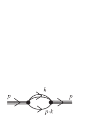
Figure 1: A diagrammatic representation of the baryon self-energies. The single, double and triple lines represent the quark, diquark and baryon respectively. The blobs represent the three point quark-diquark-baryon interactions.

With the three momentum cutoff, $\Sigma_{S}$ and $\Sigma_{A}$ are decomposed into Lorentz scalar and vector $(\gamma^{0})$ parts as

$$\Sigma_{S}(p_{0})-\frac{1}{|\hat{G}|}G_{A} = Z_{S}^{-1}(p_{0}\gamma^{0}-a_{S}),$$ (35)

$$\Sigma_{A}(p_{0})-\frac{1}{|\hat{G}|}G_{S} = Z_{A}^{-1}(p_{0}\gamma^{0}-a_{A}),$$ (36)

where we employ the baryon rest frame $p_{\mu}=(p_{0},\ \vec{0})$. The bare baryon fields $B_{1,2}$ are now renormalized as

$$\left(\begin{array}[]{c}B_{1}\\ B_{2}\end{array}\right)=\left(\begin{array}[]{c}\sqrt{Z_{S}}B_{1}^{\prime}\\ \sqrt{Z_{A}}B_{2}^{\prime}\end{array}\right),$$ (41)

with which the Lagrangian (32) is reduced to

$${\cal L}=\bar{B}^{\prime}(p_{0}\gamma^{0}-\hat{M})B^{\prime}\,.$$ (42)

Here the mass matrix $\hat{M}$ is given as

$$\hat{M}=\left(\begin{array}[]{cc}a_{S}&-\sqrt{Z_{S}Z_{A}}\frac{v}{|\hat{G}|}\\ -\sqrt{Z_{S}Z_{A}}\frac{v}{|\hat{G}|}&a_{A}\end{array}\right).$$ (45)

When there is no mixing interaction $(v=0)$, $B_{1,2}^{\prime}$ become the physical states with $a_{S}$ and $a_{A}$ being their masses. In the presence of the mixing, the physical states are obtained by the diagonalization of the mass matrix with an unitary transformation:

$$B^{\prime}=U^{\dagger}N,\;U\hat{M}U^{\dagger}=\mbox{diag}(M_{1},\;M_{2}).$$ (46)

Finally, Eq. (42) becomes

$${\cal L}=\bar{N_{1}}(p_{0}\gamma^{0}-M_{1})N_{1}+\bar{N_{2}}(p_{0}\gamma^{0}-M_{2})N_{2},$$ (47)

where the eigenvalues $M_{1,2}$ and eigenvectors $N=(N_{1},\ N_{2})^{T}$ are obtained as

$$M_{1,2} = \frac{1}{2}\left[a_{S}+a_{A}\pm\sqrt{(a_{S}-a_{A})^{2}+4Z_{S}Z_{A}\left(\frac{v}{|\hat{G}|}\right)^{2}}\;\right]\,,$$ (48)

$$N_{1} = \cos\phi B_{1}^{\prime}+\sin\phi B_{2}^{\prime}$$ (49)

$$N_{2} = -\sin\phi B_{1}^{\prime}+\cos\phi B_{2}^{\prime}\,,$$ (50)

and the mixing angle $\phi$ is given by

$$\tan\phi=\frac{|\hat{G}|\sqrt{Z_{S}Z_{A}}(a_{S}-M_{1})}{v}\,.$$ (51)

Eq. (48) should be read as a self-consistent equation where the quantities on the right hand side are functions of $M_{1,2}$. The equations are then equivalent to the Schrödinger equation for the quark-diquark system interacting through the delta function type interaction with a suitable cutoff.

2.3 Electromagnetic couplings of the nucleon and Roper resonance

We proceed to the electromagnetic terms obtained from the first term of Eq. (26) and second one of Eq. (27),

$${\cal L}_{BB\gamma} = -\bar{B}^{\prime}(p^{\prime})\left(\begin{array}[]{cc}\Lambda_{S}^{\mu}(q)&0\\ 0&\Lambda_{A}^{\mu}(q)\end{array}\right)B^{\prime}(p)A_{\mu}(q),$$ (54)

where $\Lambda_{S}(q)$ and $\Lambda_{A}(q)$ are the electromagnetic form factors of $B_{1}^{\prime}$ and $B_{2}^{\prime}$, respectively. Each of them consists of the contributions from quark-photon and diquark photon couplings, as shown in Fig. 2,

$$\Lambda_{S}^{\mu}(q) = \Lambda_{Sq}^{\mu}(q)+\Lambda_{SD}^{\mu}(q),$$ (55)

$$\Lambda_{A}^{\mu}(q) = \Lambda_{Aq}^{\mu}(q)+\Lambda_{AD}^{\mu}(q).$$ (56)

Their Feynman integrals are given by,

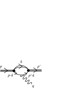
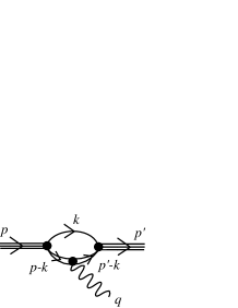
Figure 2: The electromagnetic couplings of the baryons. The left and right panels show the contribution from the quark and diquarks.

$$\Lambda_{Sq}^{\mu}(q) = iQ_{q}N_{c}Z_{S}\int\frac{d^{4}k}{(2\pi)^{4}}\Delta_{0}(k)S_{0}(p^{\prime}-k)\gamma^{\mu}S_{0}(p-k),$$ (57)

$$\Lambda_{SD}^{\mu}(q) = -iQ_{S}N_{c}Z_{S}\int\frac{d^{4}k}{(2\pi)^{4}}\Delta_{0}(p^{\prime}-k)\Gamma^{\mu}_{S}(p,\;p^{\prime})\Delta_{0}(p-k)S_{0}(k),$$ (58)

$$\Lambda_{Aq}^{\mu}(q) = \frac{3}{2}iN_{c}Z_{A}(\tau_{0}-\tau_{3})\int\frac{d^{4}k}{(2\pi)^{4}}\Delta_{0}^{\alpha\beta}(k)\gamma_{\alpha}\gamma_{5}S_{0}(p^{\prime}-k)\gamma^{\mu}S_{0}(p-k)\gamma_{\beta}\gamma_{5},$$

$$\Lambda_{AD}^{\mu}(q) = 3iN_{c}Z_{A}(\tau_{0}+2\tau_{3})$$

$$\times \int\frac{d^{4}k}{(2\pi)^{4}}\Delta_{0\alpha\beta}(p^{\prime}-k)(-\Gamma_{A}^{\beta\gamma\mu}(p,\;p^{\prime}))\Delta_{0\gamma\delta}(p-k)\gamma^{\alpha}\gamma_{5}S_{0}(k)\gamma^{\delta}\gamma^{5}.$$

where $p$ and $p^{\prime}$ are the four-momentum of $B^{\prime}_{1,2}$ in the initial and final states, and $q=p^{\prime}-p$ is the four-momentum transfer carried by the photon. Note that each $B^{\prime}_{1,2}$ is an isodoublet having two components: the charge $+1$ and $0$. Then $\tau_{0}$ and $\tau_{3}$ describe the iso-scalar and iso-vector form factors.

For the computation of the form factors at finite momentum transfer $q\neq 0$, we employ the Breit frame defined by $p^{\prime}=(p_{0},\;\vec{q}/2),\;p=(p_{0},\;-\vec{q}/2),\;q=(0,\vec{q})$. The form factors $\Lambda^{\mu}_{\alpha},\;(\alpha=Sq,\;SD,\;Aq,\;AD)$ are decomposed into the electric form factors $\Lambda^{0}_{\alpha}(q)=\Lambda^{E}_{\alpha}({\vec{q}}^{\,2})\gamma^{0}$, and the magnetic form factors $\Lambda^{i}_{\alpha}(q)=\Lambda^{M}_{\alpha}({\vec{q}}^{\,2})i\epsilon_{ijk}\sigma_{j}q_{k}\;(i=1,\;2,\;3)$. Then Eq. (54) is reduced to

$${\cal L}_{BB\gamma}= - \bar{B}^{\prime}(p^{\prime})\left(\begin{array}[]{cc}\Lambda_{S}^{E}({\vec{q}}^{\,2})&0\\ 0&\Lambda_{A}^{E}({\vec{q}}^{\,2})\end{array}\right)\gamma^{0}B^{\prime}(p)A_{0}$$ (63)

$$- \bar{B}^{\prime}(p^{\prime})\left(\begin{array}[]{cc}\Lambda_{S}^{M}({\vec{q}}^{\,2})&0\\ 0&\Lambda_{A}^{M}({\vec{q}}^{\,2})\end{array}\right)i\epsilon_{ijk}\sigma_{j}q_{k}B^{\prime}(p)A_{i}.$$ (66)

By the unitary transformation Eq.(46), we obtain the electromagnetic couplings of the nucleon and Roper resonance as

$${\cal L}_{NN\gamma}=-\bar{N}(p^{\prime})F^{E}({\vec{q}}^{\,2})\gamma^{0}N(p)A_{0}-\bar{N}(p^{\prime})F^{M}({\vec{q}}^{\,2})i\epsilon_{ijk}\sigma_{j}q_{k}N(p)A_{i},$$ (67)

where $F^{E,M}$ are defined by the unitary transformation of Eq. (66):

$$F^{E,M}({\vec{q}}^{\,2}) = U\left(\begin{array}[]{cc}\Lambda_{S}^{E,M}(\vec{q}^{\,2})&0\\ 0&\Lambda_{A}^{E,M}(\vec{q}^{\,2})\end{array}\right)U^{\dagger}_{,}$$ (70)

$$= \left(\begin{array}[]{cc}\Lambda_{S}^{E,M}\cos^{2}\phi+\Lambda_{A}^{E,M}\sin^{2}\phi&(\Lambda_{A}^{E,M}-\Lambda_{S}^{E,M})\sin\cos\phi\\ (\Lambda_{A}^{E,M}-\Lambda_{S}^{E,M})\sin\cos\phi&\Lambda_{S}^{E,M}\sin^{2}\phi+\Lambda_{A}^{E,M}\cos^{2}\phi\end{array}\right)_{.}$$ (73)

Eq. (73) is the $2\times 2$ matrix in the nucleon-Roper space, and each element is also a $2\times 2$ matrix in iso-doublet space. Therefore, Eq. (73) describes the electromagnetic properties of the four particles: the nucleon ($p$ and $n$), and the Roper resonance ($p^{*}$ and $n^{*}$), where $p$ and $p^{*}$ have the charges $+1$ and $n$ and $n^{*}$ have $0$. Thus the diagonal elements describe the form factors of them, while the off-diagonal ones their transitions. In the present paper, we shall study the diagonal components. The off-diagonal terms should be calculated in other frame, for instance the Roper-rest-frame.

It is convenient to redefine the form factors as

$$\Lambda_{Sq}^{\mu}(q) \to Q_{q}\Lambda_{Sq}^{\mu},$$ (74)

$$\Lambda_{SD}^{\mu}(q) \to Q_{S}\Lambda_{SD}^{\mu},$$ (75)

$$\Lambda_{Aq}^{\mu}(q) \to \frac{3}{2}(\tau_{0}-\tau_{3})\Lambda_{Aq}^{\mu},$$ (76)

$$\Lambda_{AD}^{\mu}(q) \to 3(\tau_{0}+2\tau_{3})\Lambda_{AD}^{\mu}.$$ (77)

Then, the electric form factors of the proton and neutron are given as,

$$G_{p}^{E}({\vec{q}}^{\,2}) = \left[\frac{2}{3}\Lambda^{E}_{Sq}({\vec{q}}^{\,2})+\frac{1}{3}\Lambda^{E}_{SD}({\vec{q}}^{\,2})\right]\cos^{2}\phi+\left[0\cdot\Lambda^{E}_{Aq}({\vec{q}}^{\,2})+\Lambda^{E}_{AD}({\vec{q}}^{\,2})\right]\sin^{2}\phi,$$

$$G_{n}^{E}({\vec{q}}^{\,2}) = \left[-\frac{1}{3}\Lambda^{E}_{Sq}({\vec{q}}^{\,2})+\frac{1}{3}\Lambda^{E}_{SD}({\vec{q}}^{\,2})\right]\cos^{2}\phi+\left[\frac{1}{3}\Lambda^{E}_{Aq}({\vec{q}}^{\,2})-\frac{1}{3}\Lambda^{E}_{AD}({\vec{q}}^{\,2})\right]\sin^{2}\phi.$$

Those of the Roper resonance are obtained by the substitution of $\sin\phi\leftrightarrow\cos\phi$. The magnetic form factors of the proton and neutron are given by,

$$\frac{G_{p}^{M}({\vec{q}}^{\,2})}{2M_{N}} = \left[\frac{2}{3}\Lambda^{M}_{Sq}({\vec{q}}^{\,2})+\frac{1}{3}\Lambda^{M}_{SD}({\vec{q}}^{\,2})\right]\cos^{2}\phi+\left[0\cdot\Lambda^{M}_{Aq}({\vec{q}}^{\,2})+\Lambda^{M}_{AD}({\vec{q}}^{\,2})\right]\sin^{2}\phi,$$

$$\frac{G_{n}^{M}({\vec{q}}^{\,2})}{2M_{N}} = \left[-\frac{1}{3}\Lambda^{M}_{Sq}({\vec{q}}^{\,2})+\frac{1}{3}\Lambda^{M}_{SD}({\vec{q}}^{\,2})\right]\cos^{2}\phi+\left[\frac{1}{3}\Lambda^{M}_{Aq}({\vec{q}}^{\,2})-\frac{1}{3}\Lambda^{M}_{AD}({\vec{q}}^{\,2})\right]\sin^{2}\phi.$$

Again, those of the Roper resonance are obtained by the substitution of $\sin\phi\leftrightarrow\cos\phi$ and $M_{N}\to M_{R}$.

2.4 Intrinsic Properties of Diquarks

The form factors are defined with the point-like diquarks. It is natural that the diquarks have intrinsic structures. First, the axial-vector diquark may have an anomalous magnetic moment, which was already introduced in Eq. (16). In addition both the diquarks have intrinsic form factors. Expressing those intrinsic form factors by $\Lambda_{I,\alpha}({\vec{q}}^{\,2}),\;(\alpha=SD,\;AD)$, they can be included by multiplying to the original ones

$$\Lambda_{\alpha}({\vec{q}}^{\,2})\to\Lambda_{\alpha}({\vec{q}}^{\,2})\Lambda_{I,\alpha}({\vec{q}}^{\,2}).$$ (82)

Here we introduce a common form factor for both the electric and magnetic terms. Then we parameterize them as,

$$\Lambda_{I,SD}({\vec{q}}^{\,2})=\frac{1}{(1+{\vec{q}}^{\,2}/b_{S})},$$ (83)

$$\Lambda_{I,AD}({\vec{q}}^{\,2})=\frac{1}{(1+{\vec{q}}^{\,2}/b_{A})^{2}},$$ (84)

We have employed the monopole and dipole shapes for the scalar and axial-vector diquarks, followed by Kroll et al. [11]. Those shapes are obtained by considering the magnetic form factors of the nucleon in high energy region. Although it is not obvious that the parameterization can be applied to the low-energy region ($\leq 1$ GeV) we are interested in, we shall employ Eqs. (84) in order to decrease the number of parameters. The values of $b_{S}$ and $b_{A}$ control the sizes of the diquarks. Explicitly the radii of the diquarks are given by

$$\langle r^{2}\rangle_{S}=\frac{6}{b_{S}}_{,}$$ (85)

$$\langle r^{2}\rangle_{A}=\frac{12}{b_{A}}_{.}$$ (86)

3 Numerical Results

3.1 Masses and Parameters

For numerical calculations, we first explain the model parameters. The constituent mass of the $u,d$ quarks $m_{q}$ and the three momentum cutoff $\Lambda$ are determined in such a way that they reproduce meson properties in the NJL model [13, 14]. The masses of the diquarks may be also calculated in the NJL model [13, 15]. We choose the mass of the scalar diquark $M_{S}$=650 MeV. The mass difference $M_{A}-M_{S}$ is related to that of the nucleon and $\Delta(1232)$. Hence, we assume the mass difference $M_{A}-M_{S}=400$ MeV with the mass of the axial-vector diquark $M_{A}=1050$ MeV . The quark-diquark coupling constants $G_{S},\;G_{A}$ and $v$ are determined so as to reproduce the masses of the nucleon and Roper resonance [2]. The parameters are summarized in Table 1.

Table 1: The parameters used in this model.

$m_{q}$ $[$GeV]	$M_{S}$ [GeV]	$M_{A}$ [GeV]	$m_{N}$ [GeV]	$m_{R}$ [GeV]
0.39	0.65	1.05	0.94	1.44

$\Lambda$ [GeV]	$G_{S}$ [GeV-1]	$G_{A}$ [GeV-1]	$v$ [GeV-1]	$\phi$ [degree]
0.6	102	11.2	23.2	18.4

In the previous section, we have introduced three parameters, $b_{S}$, $b_{A}$ and $\kappa$. We employ $b_{S}=1.25$ [GeV²] with the radius of the scalar diquark $\langle r^{2}\rangle_{S}^{1/2}=0.50$ [fm] obtained in the NJL model [18]. In Ref. [18], the axial-vector diquark has the large size $1\sim 2$ [fm]. Rather we assume that the axial-vector diquark is smaller than the nucleon, and that it is larger than the scalar diquark, because there are no strong attraction between the quarks in the axial-vector diquark. Hence the axial-vector diquark size is assumed to be within a range $\langle r^{2}\rangle_{A}^{1/2}=0.6\sim 0.9$ [fm]. Within this range, we determine $\langle r^{2}\rangle_{A}^{1/2}=0.82$ [fm] with $b_{A}=0.7$, which are appropriate to reproduce the charge radii of the proton and neutron .

For the determination of $\kappa$, it turns out that it is not easy to reproduce the magnetic moments of the nucleon with a reasonable value of $\kappa$, because of the scalar dominance with the small mixing angle $\phi\sim 18^{\circ}$. Then, we shall qualitatively investigate the effects of $\kappa$ to the magnetic moments with employing $\kappa=2$, which is larger than the values used in Kroll et al.

3.2 Electromagnetic Properties

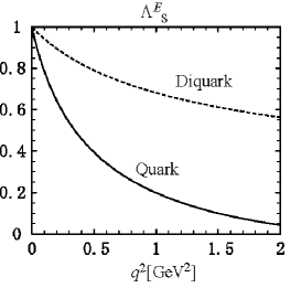
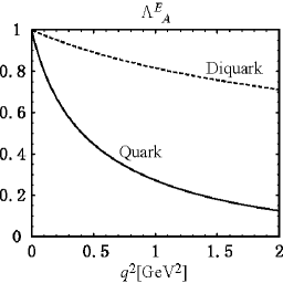
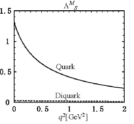
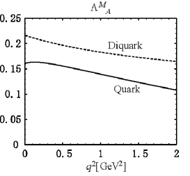
Figure 3: The eight fundamental form factors. The topped and bottomed figures show electric and magnetic form factors, where the left and right panels show the scalar and axial-vector channels. The solid and dashed lines are for the quark and diquark contributions.

The top panels of Fig. 3 show the electric form factors $\Lambda^{E}_{Sq,Aq,SD,AD}$. Here we do not include the intrinsic diquark form factors, hence the figures show the distributions of the orbital motion of the quark and diquarks. In both the scalar (left panel) and the axial-vector (right) channels, the quark contributions $\Lambda^{E}_{Sq,Aq}$ have larger $\vec{q}^{\;2}$-dependence than the diquarks $\Lambda^{E}_{SD,AD}$. In addition, the quarks have almost the same distributions in the scalar and axial-vector channels. This is understood from the system of a lighter quark and a heavier diquark, where the quark moves further from the center of mass than the diquarks. Since the quark-scalar diquark and quark-axial-vector diquark bound states have the same binding energy 50 MeV, the quarks have the similar spatial distributions and kinetic energies. As for the diquark contributions, the scalar diquarks have larger $\vec{q}^{\;2}$-dependence than the axial-vector diquarks, however both of them are almost negligible. The bottom panels of Fig. 3 show the magnetic form factors of $\Lambda^{M}_{Sq,Aq,SD,AD}$. The magnetic moments are dominated by $F^{M}_{Sq}$, while the other contributions are rather small, which is consistent with the Faddeev equation by Mineo et. al [6].

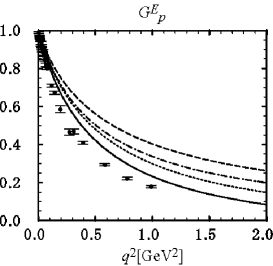
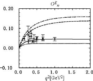
Figure 4: The electric form factors of the proton (left) and neutron (right). The dotted, dotted-dashed, solid and dashed lines are for the cases (i), (ii), (iii) and (iv). The experimental data are taken from [25, 26].

Figures 4 show the electric form factors of the proton and neutron. To see the effects of the intrinsic diquark form factors, we consider the following four cases; case (i) include the intrinsic form factor only for the scalar diquark, case (ii) only for the axial-vector diquark, case (iii) for both the diquarks and case (iv) for neither the scalar nor axial-vector diquarks. The intrinsic form factor of the scalar diquark improves both $G^{E}_{p}$ and $G^{E}_{n}$, while that of the axial-vector diquark improves $G^{E}_{p}$ but $G^{E}_{n}$. Including both the scalar and axial-vector diquark form factors, we obtain the reasonable results both for $G^{E}_{p}$ and $G^{E}_{n}$ in the region $0\leq\vec{q}^{\;2}\leq 1$ [GeV²].

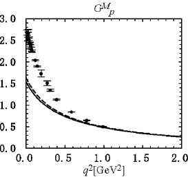
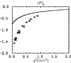
Figure 5: The magnetic form factors of the proton (left) and neutron (right). The solid and dashed lines are for $\kappa=0$ and $\kappa=2$. The experimental data are taken from [25, 27].

Figures 5 plot the magnetic form factors of the proton and neutron. Here we qualitatively estimate the effects of the anomalous magnetic moment $\kappa$ of the axial-vector diquark by considering two cases; one is a result with $\kappa=0$ and the other is with $\kappa=2$. For both cases, the intrinsic diquark form factors are included. We find that the magnetic moments of the proton and neutron are underestimated even if we include the anomalous magnetic moment: $\mu_{p}=1.6$ (exp. $2.8$), $\mu_{n}=-0.76$ $(-1.9)$ for $\kappa=2$. The deficiency is mostly found in the iso-vector magnetic moments: $\mu_{S}=0.42$ (exp. $0.44)$ and $\mu_{V}=1.2$ $(2.4)$. It is caused by the ratio of the weight factors $\cos^{2}\phi:\sin^{2}\phi=9:1$ due to the small mixing angle $\phi=18^{\circ}$. Since the magnetic moments of the nucleon are dominated by the scalar channels, the anomalous magnetic moment of the axial-vector diquark does not contribute $\mu_{p,n}$ largely .

Mineo et al. showed that the electromagnetic transition vertex between the scalar and axial-vector diquarks enhanced the magnetic moments around $2.3$ for proton and $-1.5$ for neutron. They also showed that the remaining deficiencies were supplied by the effect of the pion . Similar results were also obtained in the covariant quark-diquark model by Oettel et al. [22]. We can expect that the transition vertex contributes the magnetic moments largely, because the contribution of the transition vertex appear with a factor $\sin\phi\cos\phi$. In addition, the transition vertex contributes only to the iso-vector magnetic moment, where the deficiency is observed in our results.

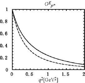
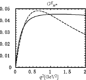
Figure 6: The electric form factors of the Roper resonance, $p^{*}$ (left) and $n^{*}$ (right). For a reference, the dashed lines are for the proton and neutron. We employ $b_{S}=0.96,\;b_{A}=0.7$ [GeV²].

Now we proceed to the Roper resonance. Figures 6 show the electric form factors of the Roper resonance. The slope of $p^{*}$ at $\vec{q}^{\;2}=0$ is comparable to that of the proton, precisely the slope of $p^{*}$ is slightly larger than that of $p$. Therefore the charge radius of $p^{*}$ is larger than that of $p$. This is understood from that the charge radius of $p$ is dominated by the orbital motion of the quark in the scalar channel, while that of $p^{*}$ is dominated by the intrinsic size of the axial-vector diquark owing to the small mixing angle and negligible orbital motion of the diquarks. For the neutron component (right panel), the charge radius of $n^{*}$ are almost same value as that of $n$. For the charge radius of $n$, the orbital motion of quark with the charge $+1/3$ and the intrinsic size of the scalar diquark with $-1/3$ almost cancel, however the former is slightly larger than the latter. Owing to this cancellation, the charge radius of $n$ become negative. There is also similar cancellation for the charge radius of $n^{*}$. In this case, however, the intrinsic size of the axial-vector diquark is slightly larger than the orbital motion of the quarks. Hence the charge radius of $p^{*}$ becomes negative. We note that the charge radius of $n^{*}$ is sensitive to the intrinsic size of the axial-vector diquark, as shown in Table 2, which is also understood from the cancellation mechanism explained above.

Table 2: The charge radii for various values of $b_{A}$, where $b_{S}$=0.96 [GeV²].

$b_{A}$ [GeV2]	$\langle r^{2}\rangle^{1/2}_{p}$ [fm]	$\langle r^{2}\rangle^{1/2}_{p^{*}}$ [fm]	$\langle r^{2}\rangle_{n}$ [fm2]	$\langle r^{2}\rangle_{n^{*}}$ [fm2]	$\langle r^{2}\rangle^{1/2}_{A}$ [fm]
$0.7$	0.75	0.84	-0.074	-0.046	0.82
$1$	0.74	0.73	-0.067	0.013	0.68
$1.3$	0.73	0.68	-0.065	0.036	0.60

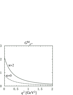
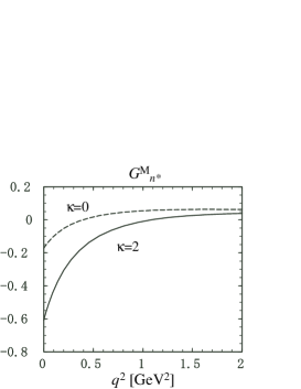
Figure 7: The magnetic form factors of the Roper resonance, $p^{*}$ (left) and $n^{*}$ (right). The solid and dashed lines are for $\kappa=2$ and $\kappa=0$. We employ $b_{S}=0.96,\;b_{A}=0.7$ [GeV²].

Figures 7 show the magnetic form factors of the Roper resonance. We also consider the following two cases: $\kappa=0$ and $\kappa=2$. The magnetic moments of the Roper are affected largely by the value of $\kappa$, in contrast to the case of the nucleon, as is easily understood from the axial-vector dominance of the Roper resonance. In the case $\kappa=0$, the magnetic moments of the Roper resonance is smaller than those of the nucleon, while in the case $\kappa=2$ the strengths of them are reversed. Now, we discuss the effects of $\kappa$. As we have explained we can obtain larger values of $\mu_{p,n}$ by employing the larger values of $\kappa$. In this case the magnetic moments of the Roper become extremely large. Hence, we can not determine the value of $\kappa$ at this moment, because there are no experimental data for the magnetic moments of the Roper resonance. Again, we expect several effects for the magnetic moments: the scalar-axial-vector diquark transition vertex, the pionic effect and so on. The determination of $\kappa$ should be done by including such effects and by reproducing the proton and neutron magnetic moments. Qualitatively, note that the magnetic moments of the nucleon and Roper can have different values. In the radial or collective excitation picture, they have the same amount of the magnetic moments, since the nucleon and Roper resonance have the same flavor wave-function. In the quark-diquark picture, the Roper has different diquark components from the nucleon. Hence the magnetic moments of the Roper differ from those of the nucleon by the effects of the (difference of) diquark correlations. Finally, Table 3 summarize the properties of the nucleon and Roper resonance.

Table 3: The charge $Q$, magnetic moment $\mu$ and charge radius $\langle r^{2}\rangle$ of $p,\;n,\;p^{*}$ and $n^{*}$. The experimental values are in the bracket. We employed $b_{S}=0.96,\;b_{A}=0.7$ [GeV²].

	$p$	$n$	$p^{*}$	$n^{*}$
$Q$	$1$	$0$	$1$	$0$
$\mu(\kappa=0)$	$1.5(2.79)$	$-0.73(-1.91)$	$0.82$	$-0.172$
$\mu(\kappa=2)$	$1.6(2.79)$	$-0.76(-1.91)$	$2.1$	$-0.61$
$\langle r^{2}\rangle^{1/2}_{E}$ [fm]	$0.75(0.86)$	-	$0.84$	-
$\langle r^{2}\rangle_{E}$ [fm2]	-	$-0.074(-0.12)$	-	-$0.046$

4 Summary and conclusion

We discussed the electromagnetic properties of the nucleon and Roper resonance in the chiral quark-diquark model. We showed that the mass difference between the nucleon and Roper resonance was reproduced by the difference of the diquark correlations between the scalar and axial-vector channels. Thus the appearance of the Roper resonance and its excitation energy is generated by the violation of the spin-flavor symmetry caused by the diquark correlation. In the present study, we employed the quark-diquark model in order to realize this scenario, however we should note that the violation of the spin-flavor symmetry is not restricted to the quark-diquark model, hence the present study can be applied to other approaches.

With the intrinsic form factors of the scalar and axial-vector diquarks we reproduced the reasonable values of the charge radii both of the proton and neutron. On the other hand, we obtained the smaller values of the magnetic moments of them than the experimental values due to the small mixing angle. The deficiencies were mostly observed in the iso-vector magnetic moments. We expect that these deficiencies are compensated by the inclusion of the electromagnetic transition vertex between the scalar and axial-vector diquarks and of the pionic effects, as suggested by Mineo et al [6]. The pion cloud probably affects both the electric and magnetic form factors, then the present picture for the nucleon and Roper resonance should be considered as their core part.

We investigated the electric form factors of the nucleon and Roper resonance, where we employ several values for the axial-vector diquark size from $\langle r^{2}\rangle_{A}^{1/2}$=0.6 $\sim$0.8 [fm]. For the proton components, the charge radii of the $p^{*}$ and $p$ are almost the same size and it is less sensitive to the diquark size. While the charge radii of $n^{*}$ is sensitive to the value of $\langle r^{2}\rangle_{A}^{1/2}$. When we employ $\langle r^{2}\rangle_{A}^{1/2}$=0.82 [fm], the charge radii of $n^{*}$ is almost comparable with those of the nucleon both for the proton and neutron components.

In conventional picture of the collective excitation of the Roper resonance, the charge radii of the Roper resonance are larger than those of the nucleon both for the proton and neutron component. In the quark-diquark picture, the Roper resonance is a spin-partner of the nucleon with the different spin component. In this case the charge radius of the Roper resonance is smaller than those in the collective picture.

References

- [1] A. Selem and F. Wilczek, arXiv:hep-ph/0602128 ; R. L. Jaffe, Phys. Rept. 409, 1 (2005) [Nucl. Phys. Proc. Suppl. 142, 343 (2005)] [arXiv:hep-ph/0409065] ; R. L. Jaffe and F. Wilczek, Phys. Rev. Lett. 91, 232003 (2003) ; M. Anselmino, E. Predazzi, S. Ekelin, S. Fredriksson and D. B. Lichtenberg, Rev. Mod. Phys. 65, 1199 (1993).
- [2] K. Nagata and A. Hosaka, J. Phys. G 32, 777 (2006).
- [3] L. Y. Glozman and D. O. Riska, Phys. Rept. 268, 263 (1996).
- [4] G. E. Brown, J. W. Durso and M. B. Johnson, Nucl. Phys. A 397, 447 (1983) ; T. Hatsuda, Nucl. Phys. A 458, 583 (1986) ; J. D. Breit and C. R. Nappi, Phys. Rev. Lett. 53, 889 (1984) ; A. Hayashi, G. Eckart, G. Holzwarth and H. Walliser, Phys. Lett. B 147, 5 (1984) ; I. Zahed, U. G. Meissner and U. B. Kaulfuss, Nucl. Phys. A 426, 525 (1984) ; M. P. Mattis and M. E. Peskin, Phys. Rev. D 32, 58 (1985) ; A. Hosaka and H. Toki, Z. Phys. A 330, 111 (1988).
- [5] A. Hosaka, M. Takayama and H. Toki, Nucl. Phys. A 678, 147 (2000).
- [6] H. Mineo, W. Bentz, N. Ishii and K. Yazaki, Nucl. Phys. A 703, 785 (2002).
- [7] L. J. Abu-Raddad, A. Hosaka, D. Ebert and H. Toki, Phys. Rev. C 66, 025206 (2002).
- [8] K. Nagata and A. Hosaka, Prog. Theor. Phys. 111, 857 (2004).
- [9] K. Nagata, A. Hosaka and L. J. Abu-Raddad, Phys. Rev. C 72, 035208 (2005) [Erratum-ibid. C 73, 049903 (2006)].
- [10] K. Nagata, A. Hosaka and V. Dmitrasinovic, arXiv:0705.1896 [hep-ph].
- [11] P. Kroll, T. Pilsner, M. Schurmann and W. Schweiger, Phys. Lett. B 316, 546 (1993).
- [12] J. He and Y. b. Dong, J. Phys. G 32, 189 (2006).
- [13] U. Vogl and W. Weise, Prog. Part. Nucl. Phys. 27, 195 (1991).
- [14] T. Hatsuda and T. Kunihiro, Phys. Rept. 247, 221 (1994).
- [15] R. T. Cahill, C. D. Roberts and J. Praschifka, Phys. Rev. D 36, 2804 (1987).
- [16] K. Orginos, PoS LAT2005, 054 (2006) [arXiv:hep-lat/0510082].
- [17] M. Hess, F. Karsch, E. Laermann and I. Wetzorke, Phys. Rev. D 58, 111502 (1998).
- [18] C. Weiss, A. Buck, R. Alkofer and H. Reinhardt, Phys. Lett. B 312, 6 (1993).
- [19] C. Alexandrou, Ph. de Forcrand and B. Lucini, Phys. Rev. Lett. 97, 222002 (2006).
- [20] A. Hosaka and H. Toki, Phys. Rept. 277, 65 (1996).
- [21] A. W. Thomas, Adv. Nucl. Phys. 13, 1 (1984).
- [22] M. Oettel, R. Alkofer and L. von Smekal, Eur. Phys. J. A 8, 553 (2000).
- [23] J. Szweda, L. S. Celenza, C. M. Shakin and W. D. Sun, Few Body Syst. 20, 93 (1996).
- [24] G. Hellstern, R. Alkofer, M. Oettel and H. Reinhardt, Nucl. Phys. A 627, 679 (1997).
- [25] G. Hohler, E. Pietarinen, I. Sabba Stefanescu, F. Borkowski, G. G. Simon, V. H. Walther and R. D. Wendling, Nucl. Phys. B 114, 505 (1976).
- [26] T. Eden et al., Phys. Rev. C 50, 1749 (1994) ; M. Ostrick et al., Phys. Rev. Lett. 83, 276 (1999) ; D. Rohe et al., Phys. Rev. Lett. 83, 4257 (1999) ; H. Zhu et al. [E93026 Collaboration], Phys. Rev. Lett. 87, 081801 (2001) ; G. Warren et al. [Jefferson Lab E93-026 Collaboration], Phys. Rev. Lett. 92, 042301 (2004) ; J. Bermuth et al., Phys. Lett. B 564, 199 (2003) ; J. Becker et al., Eur. Phys. J. A 6, 329 (1999) ; C. Herberg et al., Eur. Phys. J. A 5, 131 (1999).
- [27] E. E. W. Bruins et al., Phys. Rev. Lett. 75, 21 (1995) ; H. Anklin et al., Phys. Lett. B 428, 248 (1998) ; J. Golak, G. Ziemer, H. Kamada, H. Witala and W. Gloeckle, Phys. Rev. C 63, 034006 (2001) ; W. Xu et al., Phys. Rev. Lett. 85, 2900 (2000) ; G. Kubon et al., Phys. Lett. B 524, 26 (2002).