Empirical distributions of Chinese stock returns at different microscopic timescales

Abstract

We study the distributions of event-time returns and clock-time returns at different microscopic timescales using ultra-high-frequency data extracted from the limit-order books of 23 stocks traded in the Chinese stock market in 2003. We find that the returns at the one-trade timescale obey the inverse cubic law. For larger timescales (2-32 trades and 1-5 minutes), the returns follow the Student distribution with power-law tails. With the decrease of timescale, the tail becomes fatter, which is consistent with the vibrational theory.

, ,

1 Introduction

The distribution of asset price fluctuations has crucial implication on asset pricing and risk management Mantegna-Stanley-2000 , Bouchaud-Potters-2000 , Malevergne-Sornette-2006 . In the seminal paper for option pricing, Black and Scholes assume that asset prices follow geometric Brownian motion, that is, the returns are normally distributed Black-Scholes-1973-JPE . It is well-known that, for most financial assets, this assumption is merely a rude approximation at large time scale. In addition, Fama finds that the portfolio selection in a stable Paretian market is different from that in a Gaussian market Fama-1965-MS . It is natural that the distribution of returns remains a hot topic especially when huge databases recording transaction-level time series of stocks become available, which enables us to test classic theories and models in finance, such as the mixture of distributions hypothesis Clark-1973-Em .

The modeling of the distribution of price variations in financial markets can be traced back to the work of Bachelier in 1900 Bachelier-1900 . Let $S(t)$ denote the price of a security at time $t$. Bachelier submits that the price variation

$$\Delta{S}(t)=S(t)-S(t-\Delta{t})$$ (1)

is an i.i.d. variable and follows Gaussian distribution with zero mean. As pointed out by Mandelbrot Mandelbrot-1967-JB , an implicit assumption of Bachelier’s model is that the variance of $\Delta{S}(t)$ is independent of the price level $S(t)$ per se, which however contradicts empirical findings. Nowadays, the logarithmic return is usually used

$$r(t)=\ln S(t)-\ln S(t-\Delta{t})~{},$$ (2)

which is a precise approximation of the price growth rate Fama-1965-JB . In addition, investors are more sensitive to the relative price changes than the absolute changes according to the Weber-Fechner law Osborne-1959a-OR . Quite a few scholars found evidence supporting the Brownian motion model Osborne-1959a-OR , Laurent-1959-OR , Osborne-1959b-OR . This model is also called the Bachelier-Osborne model since Osborne independently rediscovered the model Fama-1965-JB .

More than half a century after Bachelier’s work, a revolutionary breakthrough was made by Mandelbrot, who introduced the Pareto-Lévy distribution to describe the tail of incomes and speculative price returns Mandelbrot-1960-IER , Mandelbrot-1961-Em , Mandelbrot-1963-IER , Mandelbrot-1963-JPE , Mandelbrot-1963-JB . The concept of Paretian market is soon accepted by mainstream financial scholars Fama-1965-JB . Using high-frequency data of the S&P 500 index, Mantegna and Stanley find that the distribution of returns can be well characterized by a truncated Lévy law Mantegna-Stanley-1995-Nature . Mathematically, the density of the Lévy distribution has a power-law decay in the tail

$$f(r)\sim r^{-(\alpha+1)}~{},$$ (3)

where $0<\alpha<2$. Pareto finds that the income distribution has a universal power-law exponent $\alpha=1.5$ Pareto-1896 , while Mandelbrot finds that the price fluctuations of cotton give $\alpha\approx 1.7$ Mandelbrot-1963-JB . For the S&P 500 index, it is found that $\alpha=1.4$ Mantegna-Stanley-1995-Nature .

In recent years, new evidence provided by Stanley’s group shows that the tail distributions of many stock indexes and stock prices for the USA markets exhibit an inverse cubic law Gopikrishnan-Meyer-Amaral-Stanley-1998-EPJB , Gopikrishnan-Plerou-Amaral-Meyer-Stanley-1999-PRE , Plerou-Gopikrishnan-Amaral-Meyer-Stanley-1999-PRE , where the power-law exponent is found to be close to $\alpha=3$. In contrast, empirical analyses for other stock markets have unveiled power law tail exponents other than the Lévy regime and the inverse cubic law. Makowiec and Gnaciński have studied the daily WIG index (the main index of Warsaw Stock Exchange in Poland) for five years and found that the distribution of return follows power-law behaviors in three parts with $\alpha$ equal to 0.76, 2.03 and 3.88 for the positive tail and 0.69, 1.83 and 3.06 for the negative tail Makowiec-Gnacinski-2001-APP . Bertram focuses on the high-frequency data of 200 most actively traded stocks in the Australian Stock Exchange in the period from 1993 to 2002, and reports that the distribution of returns has power-law tails with $\alpha>3$, which varies with different time interval $\Delta{t}$ from 10 to 60 minutes Bertram-2004-PA . Coronel-Brizio et al. analyze the daily data (1990-2004) of the Mexican Stock market index (IPC) and find that the distribution of the daily returns followed a power-law distribution with the exponent $\alpha^{+}=3.33$ (positive tail) and $\alpha^{-}=3.12$ (negative tail) by selecting a suitable cutoff value Coronel-Hernandez-2005-PA . Yan et al. investigate the daily returns of 104 stocks (76 from the Shanghai Stock Exchange and 28 from Shenzhen Stock Exchange) in the Chines stock markets in the period from 1994 to 2001 and argue that the tail exponent is $\alpha^{+}=2.44$ for the positive part and $\alpha^{-}=4.29$ for the negative part Yan-Zhang-Zhang-Tang-2005-PA . After removing the opening and close returns of high-frequency data for the Shanghai Stock Exchange Composite index, the tail exponents are much closer to $\alpha=3$ Zhang-Zhang-Kleinert-2007-PA .

There are also controversial results for some markets. An example comes from the Indian stock market. Matia et al. analyze the daily returns of 49 largest stocks in the National Stock Exchange over 8 years (1994-2002) and find that the distribution of daily returns significantly deviates from the power-law form but decays exponentially in the form of $P(r)=e^{-\beta r}$ with the decay coefficient $\beta=1.34$ for the positive tail and $\beta=1.51$ for the negative tail Matia-Pal-Salunkay-Stanley-2004-EPL . In contrast, Pan and Sinha have studied the the daily data of two stock indices (Nifty, 1990-2006 and Sensex, 1991-2006) and found the daily returns are exponentially distributed followed by power-law decay in the tails ($\alpha^{+}=3.10$ and $\alpha^{-}=3.18$ for Nifty and $\alpha^{+}=3.33$ and $\alpha^{-}=3.45$ for Sensex) Pan-Sinha-2007-arXiv . They also analyze the high-frequency data of 489 stocks containing the information about all the transactions carried out in the National Stock Exchange (NSE) for two-year period (2003-2004) and observe power-law tails with $\alpha^{+}=2.87$ and $\alpha^{-}=2.52$ for $\Delta t=5$ and $\alpha\approx 3$ for $\Delta{t}$ ranging from 10 to 60 minutes Pan-Sinha-2007-EPL .

An alternative model for the distribution of returns is the stretched exponential family, which serves as a bridge between exponential and power-law distributions Laherrere-Sornette-1998-EPJB , Sornette-2004 :

$$f(r)=\frac{c}{r_{0}}\left(\frac{r}{r_{0}}\right)^{c-1}e^{-(r/r_{0})^{c}},~{}~{}(r\geqslant 0)$$ (4)

where the distribution approaches to exponential when $c\to 1$. The stretched exponential model has a very interesting behavior when $c\to 0$. If $c(r/r_{0})^{c}\to\beta$ as $c\to 0$, then the stretched exponential density goes to a power law Malevergne-Pisarenko-Sornette-2005-QF , Malevergne-Pisarenko-Sornette-2006-AFE :

$$f(r)\sim\beta\frac{r_{0}^{\beta}}{r^{\beta+1}}~{}.$$ (5)

This framework is well verified by empirical analyses Malevergne-Pisarenko-Sornette-2005-QF , Malevergne-Pisarenko-Sornette-2006-AFE , Malevergne-Sornette-2006 .

A closely relevant issue concerns with the time scale $\Delta{t}$ defining the return. Roughly speaking, the tail distribution evolves from power law at small time scale to Gaussian at large scale Ghashghaie-Breymann-Peinke-Talkner-Dodge-1996-Nature , based on the variational theory in turbulence Castaing-Gagne-Hopfinger-1990-PD , Castaing-Gagne-Marchand-1993-PD , Castaing-Chabaud-Hebral-Naert-Peinke-1994-PB , Castaing-1994-PD . Numerous empirical studies have been performed in various stock prices and indexes, such as the S&P 500 index Gopikrishnan-Plerou-Amaral-Meyer-Stanley-1999-PRE , Silva-Prange-Yakovenko-2004-PA , Kiyono-Struzik-Yamamoto-2006-PRL , the U.S.A. common stocks Plerou-Gopikrishnan-Amaral-Meyer-Stanley-1999-PRE , the Hang Seng Index for the Hong Kong market Wang-Hui-2001-JEPB , and the KOSPI index and KOSDAQ for the Korean market Lee-Lee-2004-JKPS .

In this work, we utilize a nice database documenting the limit order flow and individual transactions of 23 Chinese stocks traded on the Shenzhen Stock Exchange (SZSE). For the Chinese stock market, only very few efforts were taken to investigate the return distributions Yan-Zhang-Zhang-Tang-2005-PA , Zhang-Zhang-Kleinert-2007-PA . To the best of our knowledge, there is no literature reporting relevant results at the transaction level. Our main finding is that the stock returns obey the inverse cubic law at the transaction level and thinner power laws at aggregated timescales. The rest of the paper is organized as follows. In Sec. 2, we describe in brief the database we use. We investigate the probability distribution of the event-time returns based on individual trades in Sec. 3.1 and trade-aggregated returns in Sec. 3.2. The probability distribution of the returns on fixed intervals of clock time is discussed in Sec. 3.3. The last section concludes.

2 Data sets

The study is based on the data of the limit-order books of 23 liquid stocks listed on the SZSE in the whole year 2003. The limit-order book records ultra-high-frequency data whose time stamps are accurate to 0.01 second including details of every event. The tickers of the 23 stocks investigated are the following: 000001 (Shenzhen Development Bank Co. Ltd: 887,741 trades), 000002 (China Vanke Co. Ltd: 509,360 trades), 000009 (China Baoan Group Co. Ltd: 447,660 trades), 000012 (CSG holding Co. Ltd: 290,148 trades), 000016 (Konka Group Co. Ltd: 188,526 trades), 000021 (Shenzhen Kaifa Technology Co. Ltd: 411,326 trades), 000024 (China Merchants Property Development Co. Ltd: 133,586 trades), 000027 (Shenzhen Energy Investment Co. Ltd: 313,057 trades), 000063 (ZTE Corporation, 265,450 trades), 000066 (Great Wall Technology Co. Ltd: 277,262 trades), 000088 (Shenzhen Yan Tian Port Holdings Co. Ltd: 97,195 trades), 000089 (Shenzhen Airport Co. Ltd: 189,117 trades), 000406 (Sinopec Shengli Oil Field Dynamic Group Co. Ltd: 271,389 trades), 000429 (Jiangxi Ganyue Expressway Co. Ltd: 117,424 trades), 000488 (Shandong Chenming Paper Group Co. Ltd: 120,097 trades), 000539 (Guangdong Electric Power Development Co. Ltd: 114,721 trades), 000541 (Foshan Electrical and Lighting Co. Ltd: 68,737 trades), 000550 (Jiangling Motors Co. Ltd: 346,176 trades), 000581 (Weifu High-Technology Co. Ltd: 93,947 trades), 000625 (Chongqing Changan Automobile Co. Ltd: 397,393 trades), 000709 (Tangshan Iron and Steel Co. Ltd: 207,756 trades), 000720 (Shandong Luneng Taishan Cable Co. Ltd: 132,233 trades), and 000778 (Xinxing Ductile Iron Pipes Co. Ltd: 157,321 trades).

In 2003, there are two kinds of auctions on the SESZ, namely the call auction and continuous double auction. The former refers to the process of one-time centralized matching of buy and sell orders accepted during a specified period, while the latter refers to the process of continuous matching of buy and sell orders on a one-by-one basis. In each trading day, opening call auction is held between 9:15a.m. and 9:30a.m., followed by continuous auction (9:30a.m.-11:30a.m. and 13:00p.m.-15:00p.m.). The orders that are not executed during opening call auction automatically enter continuous auction. The limit orders submitted and canceled are identified by numbers characterizing the aggressiveness and direction (buyer- versus seller-initiated) of orders. Specifically, the buyer-initiated (or seller-initiated) orders are differentiated into six aggressive catalogs from less aggressive to more aggressive: canceled orders, orders inside the book, orders on the same best price, orders inside the spread, filled orders, and unfilled orders Biais-Hillion-Spatt-1995-JF , Griffiths-Smith-Turnbull-White-2000-JFE , Hall-Hautsch-2006-EE . More information about the market can be found in Ref. Gu-Chen-Zhou-2007-EPJB .

3 Empirical distribution of returns

3.1 Probability distributions of event-time returns

We adopt the midprice of the best bid $b_{i}(t)$ and best ask $a_{i}(t)$ of stock $i$ as the price at time $t$ after a transaction occurs:

$$S_{i}(t)=\frac{b_{i}(t)+a_{i}(t)}{2}~{},$$ (6)

where $t$ is the event time corresponding to single trades. Indeed, the concept of event time was introduced some two score and odd years ago to study the distribution of returns Brada-Ernst-Tassel-1966-OR . We then define the event-time return after $\Delta{t}$ trades for stock $i$ as the logarithmic midprice change:

$$r_{i}(t)=\ln[S_{i}(t)/S_{i}(t-\Delta{t})]~{}.$$ (7)

In this section, we focus on $\Delta{t}=1$ trade. In order to treat all the returns for different stocks as an ensemble, we deal with standardized returns

$$g_{i}(t)=\frac{r_{i}(t)-\mu_{i}}{\sigma_{i}}~{},$$ (8)

where $\mu_{i}$ and $\sigma_{i}$ are respectively the mean and standard deviation of returns for stock $i$.

In our analysis, we treat the 23 groups of standardized returns $g_{i}(t)$ as an ensemble. The empirical probability density function $f(g)$ is estimated, as shown on the left panel of Fig. 1. We find that $f(g)$ can be well modeled by a Student density Blattberg-Gonedes-1974-JB :

$$f(g|\alpha,m,L)=\frac{\sqrt{L}\alpha^{\frac{\alpha}{2}}}{B\left(\frac{1}{2},\frac{\alpha}{2}\right)}\left[\alpha+L(g-m)^{2}\right]^{-\frac{\alpha+1}{2}}~{},$$ (9)

where $\alpha$ is the degrees of freedom parameter (or tail exponent), $m=\langle{g}\rangle$ is the location parameter, $L$ is the scale parameter, and $B(a,b)$ is the Beta function, that is, $B(a,~{}b)=\Gamma(a)~{}\Gamma(b)~{}/~{}\Gamma(a+b)$ with $\Gamma(\cdot)$ being the gamma function. By the definition of $g_{i}$, we have $\langle{g_{i}}\rangle=0$ and thus $m=\langle{g}\rangle=0$. Nonlinear least-squares regression gives $\alpha=3.1$ and $L=1.9$. The fitted curve is drawn on the left panel.

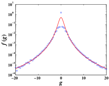
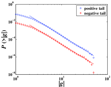
Figure 1: (Color online) Empirical distribution of event-time returns with $\Delta{t}=1$ transaction. Left: Empirical probability density function $f(g)$ of the event-time returns $g$ aggregating the 23-stock data. The solid line is the Student density with $\alpha=3.1$, $m=0$ and $L=1.9$. Right: Empirical cumulative distributions $P(g)$ for positive and negative normalized returns $g$. The solid lines are the least squares fits of power laws to the data with $\alpha^{+}=3.14\pm 0.02$ for the positive tail and $\alpha^{-}=3.00\pm 0.02$ for the negative tail.

According to the left panel of Fig. 1, the Student density fits nicely the tails of the empirical density $f(g)$. The fitted model deviates the empirical density remarkably for small values of $|g|$. For large values of $|g|$, the Student density function $f(g)$ approaches power-law decay in the tails:

$$f\left(g\right)\sim\left\{\begin{array}[]{ccc}(-g)^{-(\alpha^{-}+1)}&&{\rm{for}}~{}~{}g<0\\ (+g)^{-(\alpha^{+}+1)}&&{\rm{for}}~{}~{}g>0\end{array}\right..$$ (10)

The empirical cumulative distributions $P(g)$ of the event-time returns for positive $g$ and negative $g$ are illustrated in the right panel of Fig. 1. Both positive and negative tails decay in power-law form with $\alpha^{+}=3.14\pm 0.02$ and $\alpha^{-}=3.00\pm 0.02$ in line with the tail exponent estimated from the Student model. We note that the positive and negative tails are not asymmetric. These results indicate that the standardized returns obey the inverse cubic law.

3.2 Probability distributions of aggregated event-time returns

We now turn to investigate the distributions of aggregated event-time returns, where $\Delta{t}$ spans several trades. By varying the value of $\Delta{t}$, we are able to compare the PDF’s at different time scales. Specifically, we compare the PDFs for $\Delta{t}=2$, $4$, $8$, $16$, $32$ trades with that for $\Delta{t}=1$ trade. The empirical $f(g)$ functions averaged over 23 stocks for different time scales $\Delta{t}$ are illustrated in Fig. 2(a). We represent the distribution of one-trade return for comparison. It is evident that the tail is heavier with the decrease of $\Delta{t}$. This phenomenon can also be characterized by the kurtosis of the distributions. As listed in Table 1, the kurtosis of each PDF is significantly greater than that of the Gaussian distribution whose kurtosis is 3, indicating a much slower decay in the tails. In addition, the kurtosis decreases with respect to the scale $\Delta{t}$. We also notice that the PDF for $\Delta{t}=32$ trades decays slower than exponential.

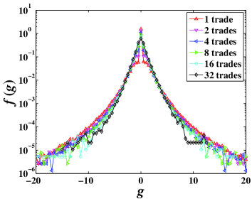
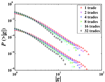
Figure 2: (Color online) Empirical distributions of aggregated event-time returns at different time scales $\Delta{t}=1,~{}2,~{}4,~{}8,~{}16,~{}32$ transactions. Panel (a): Empirical densities $f(g)$ of the aggregated event-time returns. Panel (b): Empirical cumulative distributions $P(g)$ for positive (upper cluster of curves) and negative (lower cluster of curves) returns $g$.

Table 1: Characteristic parameters for aggregated event-time returns.

	Basic statistics			Student density			Positive tail			Negative tail
$\Delta{t}$	Skewness	Kurtosis		$L$	$\alpha$		Scaling range	$\alpha^{+}$		Scaling range	$\alpha^{-}$
1	0.005	34.21		1.9	3.1		$2.4\leqslant{g}\leqslant 60.3$	$3.14\pm 0.02$		$2.1\leqslant{-g}\leqslant 60.3$	$3.00\pm 0.02$
2	0.026	26.99		1.9	3.2		$2.6\leqslant{g}\leqslant 45.7$	$3.18\pm 0.02$		$2.4\leqslant{-g}\leqslant 45.7$	$3.02\pm 0.03$
4	0.051	23.06		2.0	3.3		$2.6\leqslant{g}\leqslant 33.9$	$3.33\pm 0.03$		$2.4\leqslant{-g}\leqslant 33.9$	$3.17\pm 0.03$
8	0.106	19.53		1.9	3.5		$2.6\leqslant{g}\leqslant 25.1$	$3.63\pm 0.04$		$2.4\leqslant{-g}\leqslant 28.2$	$3.39\pm 0.04$
16	0.157	16.13		1.8	3.7		$2.6\leqslant{g}\leqslant 15.8$	$3.87\pm 0.05$		$2.4\leqslant{-g}\leqslant 19.2$	$3.50\pm 0.05$
32	0.106	13.62		1.9	4.0		$2.6\leqslant{g}\leqslant 11.9$	$4.11\pm 0.06$		$2.6\leqslant{-g}\leqslant 13.1$	$3.96\pm 0.07$

We have fitted the six curves using the Student density model (9) and the parameters $L$ and $\alpha$ are listed in Table 1. In Fig. 2(b), we study the tail distributions of the aggregated event-time returns $g$ for different time scales $\Delta{t}=2$, $4$, $8$, $16$, $32$ trades. It is observed that both positive and negative tails follow power-law distribution. We have estimated the tail exponents, which are presented in Table 1. Note that the scaling range decreases with increasing $\Delta{t}$, which is also observed for two Korean indexes Lee-Lee-2004-JKPS . As expected, the tails decay faster for larger $\Delta{t}$, which is consistent with the behavior of kurtosis. In other words, the tail exponent increases with $\Delta{t}$, which is validated by Table 1. It is interesting to note that the PDF’s for large $\Delta{t}$ deviate significantly from the inverse cubic law. We also find that $\alpha^{-}<\alpha<\alpha^{+}$, which implies that the distributions are asymmetric and is in line with the positive skewness. It seems that the sign of $\alpha^{-}-\alpha^{+}$ is not universal across different stock markets Lee-Lee-2004-JKPS .

3.3 Probability distributions of clock-time returns

In this section, we handle clock-time returns $r_{i}(t)$ defined over a fixed time interval $\Delta t$. The normalized returns $g_{i}(t)$ are calculated similarly for each stock $i$. Five different time intervals are selected with $\Delta t=1$, $2$, $3$, $4$, $5$ min. The mapping from event time to clock time is nonlinear, which is determined by the local trading frequency. The trading frequency, as a measure of stock liquidity, changes from time to time and from stock to stock. The average trading frequencies per minute for individual stocks are estimated: 15.74, 4.81, 9.03, 2.08, 7.94, 2.13, 5.14, 2.03, 3.34, 1.22, 7.29, 6.14, 2.37, 1.67, 5.55, 7.05, 4.71, 3.68, 4.92, 2.34, 1.72, 2.79, 3.35. This strongly nonlinear mapping implies that the distributions of returns in the two catalogs may behave differently.

Figure 3(a) shows the empirical probability density functions of the returns for $\Delta t=1$, $2$, $3$, $4$, $5$ minutes. We observe a nice scaling that the five density functions collapse onto a single curve when $|g|$ is less than 10, which is in agreement with the fact that the kurtosis listed in Table 2 remains unchanged approximately. This scaling is not surprising. Comparing the kurtosis listed in Table 2 with those in Table 1, it seems that the five groups of the clock-time returns are comparable to those aggregated event-time returns with $\Delta{t}=8$ to 16 trades. Indeed, the tail distributions differ from each other. We have fitted the five curves to the Student model (9) and presented the parameters $L$ and $\alpha$ in Table 2. We find that $\alpha$ increases with $\Delta{t}$, as expected. Note that these distributions decay faster than the inverse cubic law.

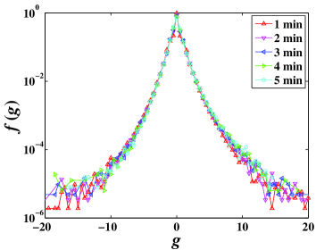
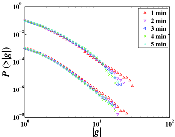
Figure 3: (Color online) Empirical distributions of clock-time returns at different time scales $\Delta t=1,~{}2,~{}3,~{}4,~{}5$ minutes. Panel (a): Empirical densities $f(g)$ of the clock-time returns. Panel (b): Empirical cumulative distributions $P(g)$ for positive (upper cluster of curves) and negative (lower cluster of curves) normalized returns $g$.

We investigate the behavior of tail distributions of the clock-time returns $g$ for different time scales $\Delta{t}=1$, $2$, $3$, $4$, $5$ min in Fig. 3(b). We found several similar characters as those for the aggregated event-time returns and the reason is possibly that when the time interval becomes large, the number of trades in this interval increases. Both the positive and negative tail exponents are estimated, which have been listed in Table 2. Again, the inequality $\alpha^{-}<\alpha<\alpha^{+}$ holds roughly.

Table 2: Characteristic parameters for clock-time returns.

	Basic statistics			Student densiy			Positive tail			Negative tail
$\Delta{t}$	Skewness	Kurtosis		$L$	$\alpha$		Scaling range	$\alpha^{+}$		Scaling range	$\alpha^{-}$
1	0.25	17.79		2.1	3.5		$2.4\leqslant{g}\leqslant 28.1$	$3.48\pm 0.02$		$2.1\leqslant{-g}\leqslant 23.2$	$3.42\pm 0.03$
2	0.51	17.70		2.2	3.6		$2.8\leqslant{g}\leqslant 23.2$	$3.70\pm 0.04$		$2.1\leqslant{-g}\leqslant 19.1$	$3.51\pm 0.04$
3	0.66	17.79		1.9	3.8		$2.8\leqslant{g}\leqslant 17.8$	$3.92\pm 0.06$		$2.4\leqslant{-g}\leqslant 17.4$	$3.58\pm 0.05$
4	0.68	18.26		1.6	3.9		$2.8\leqslant{g}\leqslant 14.4$	$4.05\pm 0.06$		$2.4\leqslant{-g}\leqslant 17.4$	$3.67\pm 0.05$
5	0.81	17.24		1.5	4.1		$2.8\leqslant{g}\leqslant 13.2$	$4.22\pm 0.07$		$2.4\leqslant{-g}\leqslant 15.8$	$3.89\pm 0.06$

4 Conclusion

Return is among the most important variables in the study of financial markets and its distribution has crucial implications in asset pricing and risk management. In this work, we have investigated a nice database constituting ultra-high-frequency data extracted from the limit-order books of 23 stocks traded on the Shenzhen Stock Exchange during the whole year of 2003. We have studied two types of returns based on event time and clock time, respectively. We find that the distributions of returns at different microscopic timescales ($\Delta{t}=1$, $2$, $4$, $8$, $16$, $32$ trades for event-time returns and $\Delta{t}=1$, $2$, $3$, $4$, $5$ minutes for clock-time returns) show power-law tails. All the distributions at different timescales can be well modeled by Student distributions with different tail exponents. For both types of returns, the tail exponent increases with the timescale $\Delta{t}$ and the exponent for the positive tail is greater than that for the negative tail at a fixed timescale. The inverse cubic law is observed only for the one-trade event-time returns.

Acknowledgments:

This work was partly supported by the National Natural Science Foundation of China (Grant no. 70501011), the Fok Ying Tong Education Foundation (Grant No. 101086), and the Shanghai Rising-Star Program (No. 06QA14015).

References

- [1] R. N. Mantegna, H. E. Stanley, An Introduction to Econophysics: Correlations and Complexity in Finance, Cambridge University Press, Cambridge, 2000.
- [2] J.-P. Bouchaud, M. Potters, Theory of Financial Risks: From Statistical Physics to Risk Management, Cambridge University Press, Cambridge, 2000.
- [3] Y. Malevergne, D. Sornette, Extreme Finanical Risks: From Dependence to Risk Management, Springer, Berlin, 2006.
- [4] F. Black, M. Scholes, The pricing of option and corporate liabilities, J. Polit. Econ. 81 (1973) 637–659.
- [5] E. F. Fama, Portfolio analysis in a stable paretian market, Management Science 11 (3) (1965) 404–419.
- [6] P. K. Clark, A subordinated stochastic process model with finite variance for speculative prices, Econometrica 41 (1) (1973) 135–155.
- [7] L. Bachelier, Théorie de la Spéculation, Ph.D. thesis, University of Paris, Paris (March 29 1900).
- [8] B. B. Mandelbrot, The variation of some other speculative prices, J. Business 40 (1967) 393–413.
- [9] E. F. Fama, The behavior of stock market prices, J. Business 38 (1) (1965) 34–105.
- [10] M. F. M. Osborne, Brownian motion in the stock market, Operations Research 7 (1959) 145–173.
- [11] A. Laurent, Comments on “Brownian motion in the stock market”, Operations Research 7 (1959) 806–807.
- [12] M. F. M. Osborne, Reply to “comments on ‘brownian motion in the stock market”’, Operations Research 7 (1959) 807–811.
- [13] B. B. Mandelbrot, The Pareto-Lévy law and the distribution of income, Int. Econ. Rev. 1 (2) (1960) 79–106.
- [14] B. B. Mandelbrot, Stable Paretian random functions and the multiplicative variation of income, Econometrica 29 (4) (1961) 517–543.
- [15] B. B. Mandelbrot, The stable Paretian income distribution when the apparent exponent is near two, Int. Econ. Rev. 4 (1) (1963) 111–115.
- [16] B. B. Mandelbrot, New methods in statistical economics, J. Polit. Econ. 71 (1963) 421–440.
- [17] B. B. Mandelbrot, The variation of certain speculative prices, J. Business 36 (1963) 394–419.
- [18] R. N. Mantegna, H. E. Stanley, Scaling behaviour in the dynamics of an economic index, Nature 376 (1995) 46–49.
- [19] V. Pareto, Cours d’economie politique, F. Rouge, Lausanne, 1896.
- [20] P. Gopikrishnan, M. Meyer, L. A. N. Amaral, H. E. Stanley, Inverse cubic law for the distribution of stock price variations, Eur. Phys. J. B 3 (1998) 139–140.
- [21] P. Gopikrishnan, V. Plerou, L. Amaral, M. Meyer, H. Stanley, Scaling of the distribution of fluctuations of financial market indices, Phys. Rev. E 60 (1999) 5305–5316.
- [22] V. Plerou, P. Gopikrishnan, L. A. N. Amaral, M. Meyer, H. E. Stanley, Scaling of the distribution of price fluctuations of individual companies, Phys. Rev. E 60 (1999) 6519–6529.
- [23] D. Makowiec, P. Gnaciński, Fluctuations of WIG-the index of Warsaw stock exchange preliminary studies, Acta Physica Polonica B 32 (2001) 1487–1500.
- [24] W. K. Bertram, An empirical investigation of Australian Stock Exchange data, Physica A 341 (2004) 533–546.
- [25] H. F. Coronel-Brizio, A. R. Hernández-Montoya, On fitting the Pareto-Levy distribution to stock market index data - Selecting a suitable cutoff value, Physica A 354 (2005) 437–449.
- [26] C. Yan, J.-W. Zhang, Y. Zhang, Y.-N. Tang, Power-law properties of Chinese stock market, Physica A 353 (2005) 425–432.
- [27] J.-W. Zhang, Y. Zhang, H. Kleinert, Power tails of index distributions in Chinese stock market, Physica A 377 (2007) 166–172.
- [28] K. Matia, M. Pal, H. Salunkay, H. E. Stanley, Scale-dependent price fluctuations for the Indian stock market, Europhys. Lett. 66 (2004) 909–914.
- [29] R. K. Pan, S. Sinha, Inverse cubic law of index fluctuation distribution in Indian markets, http://www.arxiv.org/abs/physics/0607014 (2007).
- [30] R. K. Pan, S. Sinha, Self-organization of price fluctuation distribution in evolving markets, Europhys. Lett. 5 (2007) 58004.
- [31] J. Laherrere, D. Sornette, Stretched exponential distributions in nature and economy: “Fat tails” with characteristic scales, Eur. Phys. J. B 2 (1998) 525–539.
- [32] D. Sornette, Critical Phenomena in Natural Sciences - Chaos, Fractals, Self-organization and Disorder: Concepts and Tools, 2nd Edition, Springer, Berlin, 2004.
- [33] Y. Malevergne, V. Pisarenko, D. Sornette, Empirical distributions of stock returns: Between the stretched exponential and the power law?, Quant. Finance 5 (2005) 379–401.
- [34] Y. Malevergne, V. Pisarenko, D. Sornette, On the power of generalized pareto distribution (GPD) estimators for empirical distributions of log-returns, Appl. Fin. Econ. 16 (2006) 271–289.
- [35] S. Ghashghaie, W. Breymann, J. Peinke, P. Talkner, Y. Dodge, Turbulent cascades in foreign exchange markets, Nature 381 (1996) 767–770.
- [36] B. Castaing, Y. Gagne, E. J. Hopfinger, Velocity probability density functions of high Reynolds number turbulence, Physica D 46 (1990) 177–200.
- [37] B. Castaing, Y. Gagne, M. Marchand, Log-similarity for turbulent flows?, Physica D 68 (1993) 387–400.
- [38] B. Castaing, B. Chabaud, B. Hébral, A. Naert, J. Peinke, Velocity probability density functions in developed turbulence: A finite Reynolds theory, Physica B 194-196 (1994) 695–696.
- [39] B. Castaing, Scalar intermittency in the variational theory of turbulence, Physica D 73 (1994) 31–37.
- [40] A. C. Silva, R. E. Prange, V. M. Yakovenko, Exponential distribution of financial returns at mesoscopic time lags: a new stylized fact, Physica A 344 (2004) 227–235.
- [41] K. Kiyono, Z. R. Struzik, Y. Yamamoto, Criticality and phase transition in stock-price fluctuations, Phys. Rev. Lett. 96 (2006) 068701.
- [42] B.-H. Wang, P.-M. Hui, The distribution and scaling of fluctuations for Hang Seng index in Hong Kong stock market, Eur. Phys. J. B 20 (2001) 573–579.
- [43] K. E. Lee, J. W. Lee, Scaling properties of price changes for Korean stock indices, J. Korean Phys. Soc. 44 (2004) 668–671.
- [44] B. Biais, P. Hillion, C. Spatt, An empirical analysis of the limit order book and the order flow in the Paris Bourse, J. Finance 50 (1995) 1655–1689.
- [45] M. D. Griffiths, B. F. Smith, D. A. S. Turnbull, R. W. White, The costs and determinants of order aggressiveness, J. Fin. Econ. 56 (2000) 65–88.
- [46] A. D. Hall, N. Hautsch, Order aggressiveness and order book dynamics, Emp. Econ. 30 (2006) 973–1005.
- [47] G.-F. Gu, W. Chen, W.-X. Zhou, Quantifying bid-ask spreads in the Chinese stock market using limit-order book data: Intraday pattern, probability distribution, long memory, and multifractal nature, Eur. Phys. J. B 57 (2007) 81–87.
- [48] J. Brada, H. Ernst, J. van Tassel, The distribution of stock price differences: Gaussian after all?, Operations Research 14 (2) (1966) 334–340.
- [49] R. C. Blattberg, N. J. Gonedes, A comparison of the stable and student distributions as statistical models for stock prices, J. Business 47 (2) (1974) 244–280.