Computing arithmetic invariants for hyperbolic reflection groups

Abstract

We describe a collection of computer scripts written in PARI/GP to compute, for reflection groups determined by finite-volume polyhedra in $\mathbb{H}^{3}$, the commensurability invariants known as the invariant trace field and invariant quaternion algebra. Our scripts also allow one to determine arithmeticity of such groups and the isomorphism class of the invariant quaternion algebra by analyzing its ramification.

We present many computed examples of these invariants. This is enough to show that most of the groups that we consider are pairwise incommensurable. For pairs of groups with identical invariants, not all is lost: when both groups are arithmetic, having identical invariants guarantees commensurability. We discover many “unexpected” commensurable pairs this way. We also present a non-arithmetic pair with identical invariants for which we cannot determine commensurability.

1 Introduction

Suppose that $P$ is a finite-volume polyhedron in $\mathbb{H}^{3}$ each of whose dihedral angles is an integer submultiple of $\pi$. Then the group $\Lambda(P)$ generated by reflections in the faces of $P$ is a discrete subgroup of $\mathop{\mathrm{Isom}}\nolimits(\mathbb{H}^{3})$. If one restricts attention to the subgroup $\Gamma(P)$ consisting of orientation-preserving elements of $\Lambda(P)$, one naturally obtains a discrete subgroup of $\mathop{PSL}\nolimits(2,\mathbb{C})\cong\mathop{\mathrm{Isom}}\nolimits^{+}(\mathbb{H}^{3})$. This very classical family of finite-covolume Kleinian groups is known as the family of polyhedral reflection groups.

There is a complete classification of hyperbolic polyhedra with non-obtuse dihedral angles, and hence of hyperbolic reflection groups, given by Andreev’s Theorem [3, 16] (see also [24, 14, 6] for alternatives to the classical proof); however, many more detailed questions about the resulting reflection group remain mysterious. We will refer to finite-volume hyperbolic polyhedra with non-obtuse dihedral angles as Andreev Polyhedra and finite-volume hyperbolic polyhedra with integer submultiple of $\pi$ dihedral angles Coxeter Polyhedra.

A fundamental question for general Kleinian groups is: given $\Gamma_{1}$ and $\Gamma_{2}$ does there exist an appropriate conjugating element $g\in\mathop{PSL}\nolimits(2,\mathbb{C})$ so that $\Gamma_{1}$ and $g\Gamma_{2}g^{-1}$ both have a finite-index subgroup in common? In this case, $\Gamma_{1}$ and $\Gamma_{2}$ are called commensurable. Commensurable Kleinian groups have many properties in common, including coincidences in the lengths of closed geodesics (in the corresponding orbifolds) and a rational relationship (a commensurability) between their covolumes, if the groups are of finite-covolume. See [23] for many more interesting aspects of commensurability in the context of Kleinian groups.

If $\Gamma_{1}$ and $\Gamma_{2}$ are fundamental groups of hyperbolic manifolds $M_{1}$ and $M_{2}$, commensurability is the same as the existence of a common finite-sheeted cover $\widetilde{M}$ of $M_{1}$ and of $M_{2}$. Similarly, if $\Gamma(P_{1})$ and $\Gamma(P_{2})$ are polyhedral reflection groups, they are commensurable if and only if there is a larger polyhedron $Q$ that is tiled both by $P_{1}$ under reflections in the faces (of $P_{1}$) and by $P_{2}$ under reflections in the faces (of $P_{2}$.) The existence of such a polyhedron $Q$ is clearly a fundamental and delicate question from hyperbolic geometry. See Figure 1 for an example of two commensurable polyhedra. These coordinates for these polyhedra were computed using [25] and displayed in the conformal ball model of $\mathbb{H}^{3}$ using Geomview [1].

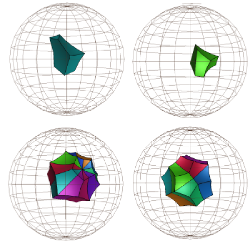
Figure 1: Two commensurable polyhedra $P_{1}$ (left top) and $P_{2}$ (right top) which tile a common larger polyhedron $Q$, here the right-angled dodecahedron.

A pair of sophisticated number-theoretic invariants has been developed by Reid and others to distinguish between commensurability classes of general finite-covolume Kleinian groups. See the recent textbook [22] and the many references therein. Given $\Gamma$, these invariants are a number field $k(\Gamma)$ known as the invariant trace field and a quaternion algebra $A(\Gamma)$ over $k(\Gamma)$ known as the invariant quaternion algebra. In fact, the invariant trace field is obtained by intersecting all of the fields generated by traces of elements of the finite-index subgroups of $\Gamma$. It is no surprise that such a field is related to commensurability because the trace of a loxodromic element $a$ of $\Gamma$ is related to the translation distance $d$ along the axis of $a$ by $2\cosh(d)={\rm Re}(tr(A))$.

The pair $\left(k(\Gamma),A(\Gamma)\right)$ does a pretty good job to distinguish commensurability classes, but there are examples of incommensurable Kleinian groups with the same $\left(k(\Gamma),A(\Gamma)\right)$. For arithmetic groups, however, the pair $\left(k(\Gamma),A(\Gamma)\right)$ is a complete commensurability invariant. Thus, one can find unexpected commensurable pairs of groups by computing these two invariants and by verifying that each group is arithmetic. See Subsection 7.7 for examples of such pairs that were discovered in this way. The precise definitions of the invariant trace field, the invariant quaternion algebra, and an arithmetic group will be given in Section 3.

It can be rather difficult to compute the invariant trace field and invariant quaternion algebra of a given Kleinian group “by hand.” However there is a beautiful computer program called SNAP [10] written by Coulson, Goodman, Hodgson, and Neumann, as described in [9]. They have computed the invariant trace field and invariant quaternion algebra, as well as many other interesting invariants, for many of the manifolds in the Hildebrand-Weeks census [12] and in the Hodgson-Weeks census [15]. The basic idea used in SNAP is to compute a high-precision decimal approximation for an ideal triangulation of the desired manifold $M$ using Newton’s Method and then to use the LLL algorithm [19] to guess exact algebraic numbers from the approximate values. These guessed values can be checked for correctness using the gluing equations describing $M$, and if the values are correct, the invariant trace field and invariant quaternion algebra can be computed from the exact triangulation.

SNAP provides a vast source of examples, also seen in the appendix of the book [22], and adds enormous flavor to the field. The fundamental techniques used in SNAP provide inspiration for our current work with polyhedral reflection groups.

In the case of polyhedral reflection groups there is a simplified description of the invariant trace field and the invariant quaternion algebra in terms of the Gram matrix of the polyhedron [21]. This theorem avoids the rather tedious trace calculations and manipulation of explicit generators of the group. Following the general technique used in the program SNAP we compute a set of outward unit normals to the faces of the polyhedron $P$ to a high decimal precision and then use the LLL algorithm to guess the exact normals as algebraic numbers. From these normals the Gram matrix is readily computed, both allowing us to check whether the guessed algebraic numbers are in fact correct, and providing the exact data needed to use the theorem from [21] in order to compute the invariant trace field and invariant quaternion algebra for $\Gamma(P)$.

Our technique is illustrated for a simple example in Section 5 and a description of our program (available to download, see [4]) is given in Section 6. Section 4 provides details on how to interpret the quaternion algebra. Finally in Section 7 we provide many results of our computations.

Acknowledgments: We thank Colin Maclachlan and Alan Reid for their beautiful work and exposition on the subject in [22]. We also thank Alan Reid for his many helpful comments.

We thank the authors of SNAP [10] and the corresponding paper [9], which inspired this project (including the choice of name for our collection of scripts). Among them Craig Hodgson has provided helpful comments.

We thank Andrei Vesnin who informed us about his result about arithmeticity of Löbell polyhedra.

We effusively thank the writers of PARI/GP [27], the system in which we have written our entire program and which is also used in SNAP [10].

The third author thanks Mikhail Lyubich and Ilia Binder for their financial support and interest in the project. He also thanks John Hubbard, to whom this volume is dedicated, for introducing him to hyperbolic geometry and for his enthusiasm for mathematics in general and experimental mathematics in particular.

2 Hyperbolic polyhedra and the Gram Matrix

We briefly recall some fundamental hyperbolic geometry, including the definition of a hyperbolic polyhedron and of the Gram matrix of a polyhedron.

Let $E^{3,1}$ be the four-dimensional Euclidean space with the indefinite metric $\|{\bf x}\|^{2}=-x_{0}^{2}+x_{1}^{2}+x_{2}^{2}+x_{3}^{2}$. Then hyperbolic space $\mathbb{H}^{3}$ is the component having $x_{0}>0$ of the subset of $E^{3,1}$ given by

$$\|{\bf x}\|^{2}=-x_{0}^{2}+x_{1}^{2}+x_{2}^{2}+x_{3}^{2}=-1$$

with the Riemannian metric induced by the indefinite metric

$$-dx_{0}^{2}+dx_{1}^{2}+dx_{2}^{2}+dx_{3}^{2}.$$

The hyperplane orthogonal to a vector ${\bf v}\in E^{3,1}$ intersects $\mathbb{H}^{3}$ if and only if $\langle{\bf v},{\bf v}\rangle>0$. Let ${\bf v}\in E^{3,1}$ be a vector with $\langle{\bf v},{\bf v}\rangle>0$, and define

$$P_{\bf v}=\{{\bf w}\in\mathbb{H}^{3}|\langle{\bf w},{\bf v}\rangle=0\}$$

to be the hyperbolic plane orthogonal to ${\bf v}$; and the corresponding closed half space:

$$H_{\bf v}^{+}=\{{\bf w}\in\mathbb{H}^{3}|\langle{\bf w},{\bf v}\rangle\geq 0\}.$$

It is a well known fact that given two planes $P_{\bf v}$ and $P_{\bf w}$ in $\mathbb{H}^{3}$ with $\langle{\bf v},{\bf v}\rangle=1$ and $\langle{\bf w},{\bf w}\rangle=1$, they:

• intersect in a line if and only if $\langle{\bf v},{\bf w}\rangle^{2}<1$, in which case their dihedral angle is $\arccos(-\langle{\bf v},{\bf w}\rangle)$.

• intersect in a single point at infinity if and only if $\langle{\bf v},{\bf w}\rangle^{2}=1$, in this case their dihedral angle is $0$.

• are disjoint if and only if $\langle{\bf v},{\bf w}\rangle^{2}>1$, in which case the distance between them is ${\rm arccosh}(-\langle{\bf v},{\bf w}\rangle))$.

Suppose that ${\bf e}_{1},\ldots,{\bf e}_{n}$ satisfy $\langle{\bf e}_{i},{\bf e}_{i}\rangle>0$ for each $i$. Then, a hyperbolic polyhedron is an intersection

$$P=\bigcap_{i=0}^{n}H_{{\bf e}_{i}}^{+}$$

having non-empty interior.

If we normalize the vectors ${\bf e}_{i}$ that are orthogonal to the faces of a polyhedron $P$, the Gram Matrix of $P$ is given by $M_{ij}(P)=2\langle{\bf e}_{i},{\bf e}_{j}\rangle$. It is also common to define the Gram matrix without this factor of $2$, but our definition is more convenient for arithmetic reasons. By construction, a Gram matrix is symmetric and has $2$s on the diagonal. Notice that the Gram matrix encodes information about both the dihedral angles between adjacent faces of $P$ and the hyperbolic distances between non-adjacent faces.

3 Invariant Trace Field, Invariant Quaternion Algebra, and Arithmeticity

The trace field of a subgroup $\Gamma$ of $\mathop{PSL}\nolimits(2,\mathbb{C})$ is the field generated by the traces of its elements; that is, $\mathbb{Q}(\mathop{\mathrm{tr}}\nolimits\Gamma):=\mathbb{Q}(\mathop{\mathrm{tr}}\nolimits\gamma:\gamma\in\Gamma)$. This field is not a commensurablitity invariant as shown by the following example found in [22].

Consider the group $\Gamma$ generated by

$$A=\left(\begin{array}[]{cc}1&1\\ 1&0\end{array}\right),\hskip 10.00002ptB=\left(\begin{array}[]{cc}1&0\\ -\omega&1\end{array}\right),$$

where $\omega=(-1+i\sqrt{3})/2$. The trace field of $\Gamma$ is $\mathbb{Q}(\sqrt{-3})$. Now let $X=\left(\begin{array}[]{cc}i&0\\ 0&-i\end{array}\right)$. It is easy to see that $X$ normalizes $\Gamma$ and its square is the identity (in $\mathop{PSL}\nolimits(2,\mathbb{C})$), so that $\Lambda=\left\langle\Gamma,X\right\rangle$ contains $\Gamma$ as a subgroup of index $2$ and is therefore commensurable with $\Gamma$. But $\Lambda$ also contains $XBA=\left(\begin{array}[]{cc}i&i\\ i\omega&-i+i\omega\end{array}\right)$, so the trace field of $\Lambda$ contains $i$ in addition to $\omega$.

The easiest way to fix this, that is, to get a commensurability invariant related to the trace field, is to associate to $\Gamma$ the intersection of the trace fields of all finite index subgroups of $\Gamma$; this is the invariant trace field denoted $k\Gamma$.

While this definition clearly shows commensurability invariance, it does not lend itself to practical calculation. The proof of Theorem 3.3.4 in [22] brings us closer: it shows that instead of intersecting many trace fields, one can look at a single one, namely, the invariant trace field of $\Gamma$ equals the trace field of its subgroup $\Gamma^{(2)}:=\langle\gamma^{2}:\gamma\in\Gamma\rangle$. (This also shows that the invariant trace field is non-trivial which is not entirely clear from the definition as an intersection.) When a finite set of generators for the group is known, this is actually enough to compute the invariant trace field. Indeed, Lemma 3.5.3 in [22] establishes that if $\Gamma=\langle\gamma_{1},\gamma_{2},\ldots,\gamma_{n}\rangle$, the invariant trace field of $\Gamma$ is generated by $\{\mathop{\mathrm{tr}}\nolimits(\gamma_{i}):1\leq i\leq n\}\cup\{\mathop{\mathrm{tr}}\nolimits(\gamma_{i}\gamma_{j}):1\leq i<j\leq n\}\cup\{\mathop{\mathrm{tr}}\nolimits(\gamma_{i}\gamma_{j}\gamma_{k}:1\leq i<j<k\leq n\}$.

For reflection groups a more efficient description can be given in terms of the Gram matrix. The description given above uses roughly $n^{3}/6$ generators for a polyhedron with $n$ faces; the following description will use only around $n^{2}/2$. But before we state it we need to define a certain quadratic space over the field $k(P):=\mathbb{Q}(a_{i_{1}i_{2}}a_{i_{2}i_{3}}\cdots a_{i_{r}i_{1}}:\{i_{1},i_{2},\ldots,i_{r}\}\subset\{1,2,\ldots,n\})$ associated to a polyhedron; this space will also appear in the next section in the theorem used to calculate the invariant quaternion algebra.

As in the previous section, given a polyhedron $P$ we will denote the outward-pointing normals to the faces by ${\bf e}_{1},\ldots,{\bf e}_{n}$ and the Gram matrix by $(a_{ij})$. Define $M(P)$ as the vector space over $k(P)$ spanned by of all the vectors of the form $a_{1i_{1}}a_{i_{1}i_{2}}\cdots a_{i_{r-1}i_{r}}{\bf e}_{i_{r}}$ where $\{i_{1},i_{2},\ldots,i_{r}\}$ ranges over the subsets of $\{1,2,\ldots,n\}$ and $n$ is the number of faces of $P$. This space $M(P)$ will be equipped with the restriction of the quadratic form with signature $(3,1)$ used in $\mathbb{H}^{3}$. We recall that the discriminant of a non-degenerate symmetric bilinear form $\langle\cdot,\cdot\rangle$ is defined as $\det\left(\langle v_{i},v_{j}\rangle\right)_{ij}$ where $\{v_{i}\}_{i}$ is a basis for the vector space on which the form is defined. The discriminant does depend on the choice of basis, but for different bases the discriminants differ by multiplication by a square in the ground field: indeed, if $u_{i}=\sum_{j}\alpha_{ij}v_{j}$, the discriminant for the basis $\{u_{i}\}_{i}$ is that of the basis $\{v_{i}\}_{i}$ multiplied by $\det(\alpha_{ij})^{2}$.

Now we can state the theorem we use to calculate the invariant trace field, Theorem 10.4.1 in [22]:

Theorem 1

Let $P$ be a Coxeter polyhedron and let $\Gamma$ be the reflection group it determines. Let $(a_{ij})$ be the Gram matrix of $P$. The invariant trace field of $\Gamma$ is $k(P)(\sqrt{d})$, where $d$ is the discriminant of the quadratic space $M(P)$ and $k(P)=\mathbb{Q}(a_{i_{1}i_{2}}a_{i_{2}i_{3}}\cdots a_{i_{r}i_{1}}:\{i_{1},i_{2},\ldots,i_{r}\}\subset\{1,2,\ldots,n\})$ is the field defined previously.

3.1 The Invariant Quaternion Algebra

A quaternion algebra over a field $F$ is a four-dimensional associative algebra $A$ with basis $\{1,i,j,k\}$ satisfying $i^{2}=a1$, $j^{2}=b1$ and $ij=ji=-k$ for some $a,b\in F$. Note that $k^{2}=(ij)^{2}=ijij=-ijji=-ab1$. The case $F=\mathbb{R}$, $a=b=-1$ gives Hamilton’s quaternions.

The quaternion algebra defined by a pair $a,b$ of elements of $F$ is denoted by its Hilbert symbol $\left(\frac{a,b}{F}\right)$. A quaternion algebra does not uniquely determine a Hilbert symbol for it, since, for example, $\left(\frac{a,b}{F}\right)=\left(\frac{a,-ab}{F}\right)=\left(\frac{au^{2},bv^{2}}{F}\right)$ for any invertible elements $u,v\in F$. Fortunately, there is a computationally effective way of deciding whether two Hilbert symbols give the same quaternion algebra. This will be discussed in Section 4; for now we will just define the invariant quaternion algebra of a subgroup of $\mathop{PSL}\nolimits(2,\mathbb{C})$ and state the theorem we use to calculate a Hilbert symbol for it.

Given any non-elementary subgroup $\Gamma$ of $\mathop{PSL}\nolimits(2,\mathbb{C})$, we can form the algebra $A_{0}\Gamma:=\{\sum a_{i}\gamma_{i}:a_{i}\in\mathbb{Q}(\mathop{\mathrm{tr}}\nolimits\Gamma),\gamma_{i}\in\Gamma\}$. (Abusing notation slightly we consider the elements of $\Gamma$ as matrices defined up to sign.) This turns out to be a quaternion algebra over the trace field $\mathbb{Q}(\mathop{\mathrm{tr}}\nolimits\Gamma)$ (see Theorem 3.2.1 in [22]).

Just as with the trace fields, we define the invariant quaternion algebra of $\Gamma$, denoted by $A\Gamma$, as the intersection of all the quaternion algebras associated to finite-index subgroups of $\Gamma$.

When $\Gamma$ is finitely generated in addition to non-elementary, we are in a situation similar to that of the invariant trace field in that the invariant quaternion algebra is simply the quaternion algebra associated to the subgroup $\Gamma^{(2)}$ of $\Gamma$, or in symbols, $A\Gamma=A_{0}\Gamma^{(2)}$. To see this, note that Theorem 3.3.5 in [22] states that for finitely generated non-elementary $\Gamma$, the quaternion algebra $A_{0}\Gamma^{(2)}$ is a commensurability invariant. Now, given an arbitrary finite-index subgroup $\Lambda$ of $\Gamma$ we have $A\Gamma\subset A_{0}\Gamma^{(2)}=A_{0}\Lambda^{(2)}\subset A_{0}\Lambda$.

In the case where $\Gamma$ is the reflection group of a polyhedron $P$, $A\Gamma$ can be identified as the even-degree subalgebra of a certain Clifford algebra associated with $P$. Let us briefly recall the basic notions related to Clifford algebras. Given an $n$-dimensional vector space $V$ over a field $F$ equipped with a non-degenerate symmetric bilinear form $\left\langle\cdot,\cdot\right\rangle$ and associated quadratic form $\left\|\cdot\right\|^{2}$, the Clifford algebra it determines is the $2^{n}$-dimensional $F$-algebra generated by all formal products of vectors in $V$ subject to the condition $v^{2}=\left\langle v,v\right\rangle 1$ (where $1$ is the empty product of vectors). If $\{v_{1},v_{2},\ldots,v_{n}\}$ is an orthogonal basis of $V$, a basis for the Clifford algebra $C(V)$ is $\{v_{i_{1}}v_{i_{2}}\cdots v_{i_{r}}:1\leq r\leq n,1\leq i_{1}<i_{2}<\cdots<i_{r}\leq n\}$. There is a $\mathbb{Z}_{2}$-grading of $C(V)$ given on monomials by the parity of the number of vector factors.

Now we can state the result mentioned above: $A\Gamma$ is the even-degree subalgebra of $C(M)$ where $M$ is the vector space over the invariant trace field of $\Gamma$ that appears in Theorem 1. This relationship between the invariant trace algebra and $M$ allows one to prove a theorem giving an algorithm for computing the Hilbert symbol for the invariant quaternion algebra, part of Theorem 3.1 in [21]:

Theorem 2

The invariant quaternion algebra of the reflection group $\Gamma$ of a polyhedron $P$ is given by

$$A\Gamma=\left(\frac{-\left\|u_{1}\right\|^{2}\left\|u_{2}\right\|^{2},-\left\|u_{1}\right\|^{2}\left\|u_{3}\right\|^{2}}{k\Gamma}\right),$$

where $\{u_{1},u_{2},u_{3},u_{4}\}$ is an orthogonal basis for the quadratic space $M(P)$ defined in the previous section.

In many cases when studying an orbifold $O=\mathbb{H}^{3}/\Gamma$, a simple observation about the singular locus of $O$ leads to the fact that the invariant quaternion algebra can represented by the Hilbert symbol $\left(\frac{-1,-1}{k\Gamma}\right)$. This happens particularly often for polyhedral reflection groups.

Any vertex in the singular locus must be trivalent and must have labels from the short list shown in Figure 2. See [5] for more information on orbifolds, and in particular page 24 from which Figure 2 is essentially copied.

Figure 2: The possible vertices in the singular locus of a $3$-dimensional orbifold. The last three have vertex stabilizer containing $A_{4}$.

The last three have vertex stabilizer containing $A_{4}$, so if $\mathbb{H}^{3}/\Gamma$ has singular locus containing such a vertex, $\Gamma$ must contain $A_{4}$ as a subgroup. In this case, the invariant quaternion algebra can be represented by the Hilbert symbol $\left(\frac{-1,-1}{k\Gamma}\right)$, see [22], Lemma 5.4.1. (See also Lemma 5.4.2.)

For a polyhedral reflection group generated by a Coxeter polyhedron $P$, the corresponding orbifold $\mathbb{H}^{3}/\Gamma$ has underlying space $\mathbb{S}^{3}$ and the singular set is (an unknotted) copy of the edge graph of $P$. The label at each edge having dihedral angle $\frac{\pi}{n}$ is merely $n$. In many cases, this simplification makes it easier to compute the Hilbert symbol of a polyhedral reflection group. We do not automate this check within our program, but it can be useful to the reader.

4 Quaternion algebras and their invariants

As mentioned before, a quaternion algebra is fully determined by its Hilbert symbol $\left(\frac{a,b}{F}\right)$, although this is by no means unique. For example,

$$\left(\frac{b,a}{F}\right),\qquad\left(\frac{a,-ab}{F}\right),\qquad\textrm{and}\qquad\left(\frac{ax^{2},by^{2}}{F}\right)$$

all determine the same algebra (here $x$ and $y$ are arbitrary invertible elements of $F$.)

Taking $F=\mathbb{R}$, the Hilbert symbol $\left(\frac{-1,-1}{\mathbb{R}}\right)$ represents the ordinary quaternions (or Hamiltonians,) denoted by $\mathcal{H}$. If $F$ is any field, the Hilbert symbol $\left(\frac{1,1}{F}\right)$ is isomorphic to $M_{2}(F)$, the two-by-two matrices over $F$.

A natural question now arises; namely, when do two Hilbert symbols represent the same quaternion algebra? This question is pertinent for us—especially in the case when $F$ is a number field—because the invariant quaternion algebra is an invariant for a reflection group. For these purposes, we will need some way of classifying quaternion algebras over number fields. All of the following material on quaternion algebras appears in the reference [22].

The first step in the classification of quaternion algebras is the following theorem:

Theorem 3

Let $A$ be a quaternion algebra over a field $F$. Then either $A$ is a division algebra or $A$ is isomorphic to $M_{2}(F)$.

In the latter case, we say that $A$ splits. There are several different ways of expressing this condition, one of which will be particularly useful for us:

Theorem 4

The quaternion algebra $A=\left(\frac{a,b}{F}\right)$ splits over $F$ if and only if the equation

$$ax^{2}+by^{2}=1$$ (1)

has a solution in $F\times F$. We call this equation the Hilbert equation of $A$.

When $F$ is a number field, it turns out that in order to classify the quaternion algebras over $F$ completely we need to look at quaternion algebras over the completions of $F$ with respect to its valuations. The first chapter of [22] contains a brief introduction to number fields and valuations, and [18] is a standard text on the subject.

Definition 5

Let $F$ be any field. A valuation on $F$ is a map $\nu:F\rightarrow\mathbb{R}^{+}$ such that

• $\nu(x)\geq 0$ for all $x\in F$ and $\nu(x)=0$ if and only if $x=0$,

• $\nu(xy)=\nu(x)\nu(y)$ for all $x,y\in F$,  and

• $\nu(x+y)\leq\nu(x)+\nu(y)$ for all $x,y\in F$.

Any field admits a trivial valuation $\nu(x)=1$ for all $x\neq 0$. When $F$ is a subfield of the real (or complex) numbers, the ordinary absolute value (or modulus) function is a valuation when restricted to $F$. In general, valuations on a field fall into two different classes.

Definition 6

If a valuation $\nu$ on a field $F$ also satisfies

• $\nu(x+y)\leq max\{\nu(x),\nu(y)\}$ for all $x,y\in F$,

then $\nu$ is called a non-Archimedean valuation. If the valuation $\nu$ does not satisfy (iv), then it is called Archimedean.

There is also a notion of equivalence between valuations.

Definition 7

Two valuations $\nu_{1}$ and $\nu_{2}$ on $F$ are called equivalent if there exists some $\alpha\in\mathbb{R}^{+}$ such that $\nu_{2}(x)=\big{(}\nu_{1}(x)\big{)}^{\alpha}$ for all $x\in F$.

When $F$ is a number field, it is possible to classify all valuations on $F$ up to this notion of equivalence. Let $\sigma$ be a real or complex embedding of $F$. Then a valuation $\nu_{\sigma}$ can be defined by $\nu_{\sigma}(x)=|\sigma(x)|$, where $|\cdot|$ is the absolute value on $\mathbb{R}$ or modulus on $\mathbb{C}$. This is an Archimedean valuation on $F$, and up to equivalence these are the only Archimedean valuations that $F$ admits.

Denote by $R_{F}$ the ring of integers of $F$—i.e. the set of elements of $F$ satisfying some monic polynomial equation with integer coefficients—which is a subring of $F$. Let $\mathcal{P}$ be a prime ideal in $R_{F}$. Define a function $n_{\mathcal{P}}:R_{F}\rightarrow\mathbb{Z}$ by $n_{\mathcal{P}}(a)=m$, where $m$ is the largest integer such that $a\in\mathcal{P}^{m}$. Since $F$ is the field of fractions of $R_{F}$, $n_{\mathcal{P}}$ can be extended to all of $F$ by the rule $n_{\mathcal{P}}(a/b)=n_{\mathcal{P}}(a)-n_{\mathcal{P}}(b)$. Now pick $c$ with $0<c<1$. The function $\nu_{\mathcal{P}}:R_{F}\rightarrow\mathbb{R}^{+}$ given by $\nu_{\mathcal{P}}(x)=c^{n_{\mathcal{P}}(x)}$ is a non-Archimedean valuation on $F$. Moreover, all non-Archimedean valuations on $F$ are equivalent to a valuation of this form.

We summarize these facts in the following theorem.

Theorem 8

Let $F$ be a number field. Then every Archimedean valuation of $F$ is equivalent to $\nu_{\sigma}$ for some real or complex embedding $\sigma$ of $F$, and every non-Archimedean valuation of $F$ is equivalent to $\nu_{\mathcal{P}}$ for some prime ideal $\mathcal{P}$ of $R_{F}$. The former are sometimes called infinite places, while the latter are called finite places.

A valuation $\nu$ on a field $F$ defines a metric on $F$ by $d(x,y)=\nu(x-y)$. The completion of $F$ with respect to this metric is denoted by $F_{\nu}$. Equivalent valuations give rise to the same completions. If $\nu=\nu_{\sigma}$ for a real or complex embedding $\sigma$ of $F$, then $F_{\nu}$ is isomorphic to $\mathbb{R}$ or $\mathbb{C}$ respectively. If $\nu=\nu_{\mathcal{P}}$ for some prime ideal $\mathcal{P}\subseteq R_{F}$, then $F_{\nu}$ is called a $\mathcal{P}$-adic field.

Let $A$ be a quaternion algebra over a number field $F$, and let $F_{\nu}$ be the completion of $F$ with respect to some valuation $\nu$. Then we can construct the tensor product $A\otimes_{F}F_{\nu}$, which turns out to be a quaternion algebra over $F_{\nu}$. Indeed, if $A=\left(\frac{a,b}{F}\right)$, then $A\otimes_{F}F_{\nu}=\left(\frac{a,b}{F_{\nu}}\right)$. Ultimately, the classification of quaternion algebras over $F$ will be reduced to the classification of quaternion algebras over completions of $F$ with respect to valuations $\nu$. The two following theorems will be useful in this regard.

Theorem 9

Let $\mathbb{R}$ be the real number field. Then $\mathcal{H}$ is the unique quaternion division algebra over $\mathbb{R}$.

Theorem 10

Let $F_{\nu}$ be a $\mathcal{P}$-adic field. Then there is a unique quaternion division algebra over $F_{\nu}$.

Thus when $A$ is a quaternion algebra over a number field $F$ and $A_{\nu}$ is the corresponding quaternion algebra over a real or $\mathcal{P}$-adic completion $F_{\nu}$ of $F$, by Theorem 3 there are two possibilities: $A$ is the unique quaternion division algebra over $F_{\nu}$, or $A\cong M_{2}(F_{\nu})$. In the former case, we say that $A$ ramifies at $\nu$, while in the latter case we say that $A$ splits at $\nu$. When $F_{\nu}=\mathbb{R}$, there is a simple test to determine which algebra is represented by the Hilbert symbol $\left(\frac{a,b}{\mathbb{R}}\right)$:

if $$a b A\cong\mathcal{H} A$$ and are both negative, then , otherwise splits. (2)

Various tests exist for $\mathcal{P}_{\nu}$, but often the simplest test is to determine if there exists a solution to equation (1). (See Appendix A.) Notice that by Theorem 4 every quaternion algebra over the complex numbers is isomorphic to $M_{2}(\mathbb{C})$.

The following theorem provides the necessary criterion for distinguishing between quaternion algebras over number fields.

Theorem 11

(Vignéras [31].) Let $F$ be a number field. For each quaternion algebra $A$ over $F$, denote by $Ram(A)$ the set of all real or finite places at which $A$ ramifies. Then two quaternion algebras $A$ and $A^{\prime}$ over $F$ are equal if and only if $Ram(A)=Ram(A^{\prime})$.

Thus the complete identification of a quaternion algebra $A$ over a number field $F$ amounts to determining $Ram(A)$. It is easy to check if $A$ ramifies at the real infinite places of $F$. Let $\alpha$ be a primitive element of $F$ (i.e. an element whose powers form a basis for $F$ over $\mathbb{Q}$.) Every embedding of $F$ in $\mathbb{R}$ can be obtained from a real root $\alpha_{i}$ of the minimal polynomial of $\alpha$ over $\mathbb{Q}$ by extending the map $\sigma_{i}:\alpha\rightarrow\alpha_{i}$ linearly to $F$. If $A=\left(\frac{a,b}{F}\right)$ and $a$ and $b$ are expressed as polynomials in $\alpha$, then it is straightforward to check if condition (2) holds for $\sigma_{i}(a)$ and $\sigma_{i}(b)$.

The finite places of $F$ are more difficult to check. The most straightforward method is to check to see if the Hilbert equation (1) has a solution; our procedure for doing this is detailed in Appendix A.

4.1 Arithmeticity

The notion of an arithmetic group comes from the theory of algebraic groups and is a standard way of producing finite-covolume discrete subgroups of semi-simple Lie groups. To see how this general theory relates to Kleinian groups, see [13] or [22].

In the case of Kleinian groups, the following definition coincides with the most general one, and is naturally related to the quaternion algebras which we have already mentioned.

Let $A$ be a quaternion algebra over a number field $F$ and denote by $R_{F}$ the ring of integers in $F$. An order ${\cal O}$ in $A$ is an $R_{F}$-lattice (spanning $A$ over $F$) that is also a ring with unity. For every complex place $\nu$ of $F$ there is an embedding of $A\longrightarrow M_{2}(\mathbb{C})$ determined by the isomorphism $A\otimes_{F}F_{\nu}\cong M_{2}(\mathbb{C})$. Given a complex place $\nu$ and an order ${\cal O}$, we can construct a subgroup of $\mathop{SL}\nolimits(2,\mathbb{C})$, and hence of $\mathop{PSL}\nolimits(2,\mathbb{C})$, by taking the image $\Gamma_{\cal O}^{\nu}$ of the elements of ${\cal O}$ with unit norm under the embedding $A\longrightarrow M_{2}(\mathbb{C})$ defined above.

In the case that $F$ has a unique complex place $\nu$ and that $A$ ramifies over every real place of $F$, then $\Gamma_{\cal O}:=\Gamma_{\cal O}^{\nu}$ is a discrete subgroup of $\mathop{PSL}\nolimits(2,\mathbb{C})$ (see Sections 8.1 and 8.2 of [22]).

Definition 12

A Kleinian group $\Gamma$ is called arithmetic if it is commensurable with $\Gamma_{\cal O}$ for some order ${\cal O}$ of a quaternion algebra that ramifies over every real place and is defined over a field with a unique complex place.

Viewing $\mathop{\mathrm{Isom}}\nolimits^{+}(\mathbb{H}^{3})$ as $SO^{+}(3,1)$ furnishes an alternative construction of arithmetic Kleinian groups as follows. Let $F$ be a real number field, and $(V,q)$ a four-dimensional quadratic space over $F$ with signature $(3,1)$. Any $F$-linear map $\sigma:V\longrightarrow V$ preserving $q$ can be identified with an element of $SO^{+}(3,1)$, and thus of $\mathop{\mathrm{Isom}}\nolimits^{+}(\mathbb{H}^{3})$, by extension of scalars from $F$ to $\mathbb{R}$. Given an $R_{F}$-lattice $L\subset V$ of rank 4 over $R_{F}$, the group $\mathop{SO}\nolimits(L):=\{\sigma\in SO^{+}(3,1)\cap GL(4,F):\sigma(L)=L\}$ is always discrete and arithmetic.

Moreover, the groups of the form $\mathop{SO}\nolimits(L)$ give representatives for the commensurability classes of all Kleinian groups that possess a non-elementary Fuchsian subgroup. Since all reflection groups determined by finite-volume polyhedra have non-elementary Fuchsian subgroups, for our purposes this can be considered the definition of arithmeticity. See [13, page 143] for a discussion. The distinction between arithmetic groups arising from quaternion algebras and those arising from quadratic forms is also discussed in [33, pages 217–221], whose authors call the latter “arithmetic groups of the simplest kind”.

Aside from its relationship to algebraic groups, arithmeticity is interesting for many reasons including the fact that for arithmetic groups $\Gamma$ the pair $(k\Gamma,A\Gamma)$ is a complete commensurability invariant (see Section 8.4 of [22]). This will allow us to identify several unexpected pairs of commensurable reflection groups which are presented in Section 7.7.

To decide whether a given reflection group $\Gamma$ determined by a polyhedron $P$ is arithmetic there is a classical theorem due to Vinberg [32]:

Theorem 13

Let $(a_{ij})$ be the Gram matrix of a Coxeter polyhedron $P$. Then the reflection group determined by $P$ is arithmetic if and only if the following three conditions hold:

1. $K:=\mathbb{Q}(a_{ij})$ is totally real.

2. For every embedding $\sigma:K\longrightarrow\mathbb{C}$ such that $\sigma|_{k(P)}\neq\mathop{\mathrm{id}}\nolimits$ (where $k(P)$ is the field defined in Theorem 1), the matrix $(\sigma(a_{ij}))$ is positive semi-definite.

3. The $a_{ij}$ are algebraic integers.

More generally, for any finite-covolume Kleinian group $\Gamma$, Maclachlan and Reid have proved a similar result, Theorem 8.3.2 in [22]:

Theorem 14

A finite-covolume Kleinian group $\Gamma$ is arithmetic if and only if the following three conditions hold:

1. $k\Gamma$ has exactly one complex place.

2. $A\Gamma$ ramifies at every real place of $k\Gamma$.

3. $tr\gamma$ is an algebraic integer for each $\gamma\in\Gamma$.

5 Worked example

A Lambert cube is a compact polyhedron realizing the combinatorial type of a cube, with three disjoint non-coplanar edges chosen and assigned dihedral angles $\frac{\pi}{l},$ $\frac{\pi}{m}$, and $\frac{\pi}{n}$, and the remaining edges assigned dihedral angles $\frac{\pi}{2}$. It is easy to verify that if $l,m,n>2$, then, such an assignment of dihedral angles satisfies the hypotheses of Andreev’s Theorem. The resulting polyhedron is called the $(l,m,n)$-Lambert Cube, which we will denote by $P_{l,m,n}$.

In this section we illustrate our techniques by computing the invariant trace field and invariant quaternion algebra associated to the $(3,3,6)$ Lambert cube.

The starting point of our computation is a set of low-precision decimal approximations of outward-pointing normal vectors $\{{\bf e}_{1},\ldots,{\bf e}_{6}\}$ to the six faces of our cube. For a given compact hyperbolic polyhedron, it is nontrivial to construct such a set of outward-pointing normal vectors. One way is to use the collection of Matlab scripts described in [25]. Throughout this paper we will always assume the following normalization for the location of our polyhedron: the first three faces meet at a vertex, the first face has normal vector $(0,0,0,*)$, the second face has normal vector $(0,0,*,*)$, and the third has form $(0,*,*,*)$, where $*$ indicates that no condition is placed on that number.

We then use Newton’s Method with extended-precision decimals to improve this set of approximate normals until they are very precise. (Here, we do this with precision $40$ numbers, but we display fewer digits for the reader.) The vectors $\{{\bf e}_{1},\ldots{\bf e}_{6}\}$ are displayed as rows in the following matrix:

$$\left[\begin{array}[]{cccc}0.0&-0.0&0.0&-0.99999996237702\\ \vskip 6.0pt plus 2.0pt minus 2.0pt\cr 0.0&0.0&0.86602540463740&0.50000001881149\\ \vskip 6.0pt plus 2.0pt minus 2.0pt\cr-0.0&-1.00000002377892&-0.0&{1.0\times 10^{-14}}\\ \vskip 6.0pt plus 2.0pt minus 2.0pt\cr 1.38941010745090&0.86602538319131&-0.73831913868376&1.27880621354777\\ \vskip 6.0pt plus 2.0pt minus 2.0pt\cr 0.79708547435960&1.27880618290479&0.0&-0.0\\ \vskip 6.0pt plus 2.0pt minus 2.0pt\cr 0.62728529885922&0.0&-1.18046043888844&{1.0\times 10^{-14}}\end{array}\right]$$

The normalization we have chosen for the location of our polyhedron assures us that each of these decimals should approximate an algebraic number of some (low) degree. There are commands in many computer algebra packages for guessing the minimal polynomial that is most likely satisfied by a given decimal approximate. Most of these commands are ultimately based on the LLL algorithm [19]. (We have used the command minpoly() in Maple, the command algdep() in Pari/GP, and the command RootApproximant[] in Mathematica 6.) Each of these commands requires a parameter specifying up to what degree of polynomials to search. In this case we specify degree $30$. The resulting matrix of guessed minimal polynomials is:

$$\left[\begin{array}[]{cccc}{\it X}&{\it X}&{\it X}&1+{\it X}\\ \vskip 6.0pt plus 2.0pt minus 2.0pt\cr{\it X}&{\it X}&-3+4\,{{\it X}}^{2}&-1+2\,{\it X}\\ \vskip 6.0pt plus 2.0pt minus 2.0pt\cr{\it X}&1+{\it X}&{\it X}&{\it X}\\ \vskip 6.0pt plus 2.0pt minus 2.0pt\cr-9-88\,{{\it X}}^{2}+48\,{{\it X}}^{4}&-3+4\,{{\it X}}^{2}&1-28\,{{\it X}}^{2}+48\,{{\it X}}^{4}&3-28\,{{\it X}}^{2}+16\,{{\it X}}^{4}\\ \vskip 6.0pt plus 2.0pt minus 2.0pt\cr-9+4\,{{\it X}}^{2}+16\,{{\it X}}^{4}&3-28\,{{\it X}}^{2}+16\,{{\it X}}^{4}&{\it X}&{\it X}\\ \vskip 6.0pt plus 2.0pt minus 2.0pt\cr-1-{{\it X}}^{2}+9\,{{\it X}}^{4}&{\it X}&-3+{\it X}+3\,{{\it X}}^{2}&{\it X}\end{array}\right]$$

The next step is to specify which root of each given minimal polynomial is closest to the decimal approximate above. In the current case, the solutions of each polynomial are easily expressed by radicals, so we merely pick the appropriate expression. (For more complicated examples, our computer program uses a more sophisticated way of expressing algebraic numbers as described in Section 6.) For the current example, the following matrix contains as rows our guessed exact values for $\{{\bf e}_{1},\ldots{\bf e}_{6}\}$.

$$N:=\left[\begin{array}[]{cccc}0&0&0&-1\\ \vskip 6.0pt plus 2.0pt minus 2.0pt\cr 0&0&\frac{\sqrt{3}}{2}&\frac{1}{2}\\ \vskip 6.0pt plus 2.0pt minus 2.0pt\cr 0&-1&0&0\\ \vskip 6.0pt plus 2.0pt minus 2.0pt\cr\frac{\sqrt{33+6\,\sqrt{37}}}{6}&\frac{\sqrt{3}}{2}&\frac{-\sqrt{42+6\,\sqrt{37}}}{12}&\frac{\sqrt{14+2\,\sqrt{37}}}{4}\\ \vskip 6.0pt plus 2.0pt minus 2.0pt\cr\frac{\sqrt{-2+2\,\sqrt{37}}}{4}&\frac{\sqrt{14+2\,\sqrt{37}}}{4}&0&0\\ \vskip 6.0pt plus 2.0pt minus 2.0pt\cr\frac{\sqrt{2+2\,\sqrt{37}}}{6}&0&\frac{-1-\sqrt{37}}{6}&0\end{array}\right]$$

Corresponding to this set of guessed normal vectors we have the Gram Matrix $G_{i,j}=2\langle{\bf e}_{i},{\bf e}_{j}\rangle$:

$$G:=\left[\begin{array}[]{cccccc}2&-1&0&\frac{-\sqrt{14+2\,\sqrt{37}}}{2}&0&0\\ \vskip 6.0pt plus 2.0pt minus 2.0pt\cr-1&2&0&0&0&\frac{-\sqrt{3}\left(1+\sqrt{37}\right)}{6}\\ \vskip 6.0pt plus 2.0pt minus 2.0pt\cr 0&0&2&-\sqrt{3}&\frac{-\sqrt{14+2\,\sqrt{37}}}{2}&0\\ \vskip 6.0pt plus 2.0pt minus 2.0pt\cr\frac{-\sqrt{14+2\,\sqrt{37}}}{2}&0&-\sqrt{3}&2&0&0\\ \vskip 6.0pt plus 2.0pt minus 2.0pt\cr 0&0&\frac{-\sqrt{14+2\,\sqrt{37}}}{2}&0&2&-1\\ \vskip 6.0pt plus 2.0pt minus 2.0pt\cr 0&\frac{-\sqrt{3}\left(1+\sqrt{37}\right)}{6}&0&0&-1&2\end{array}\right]$$

By checking that there are $2$’s down the diagonal of $G$ and that there is $-2\cos(\alpha_{ij})$ in the $ij$-th entry of $G$ if faces $i$ and $j$ are adjacent, we can see that the guessed matrix $N$ whose rows represent outward-pointing normal vectors was correct. Here there are $4\cdot 6-6=18$ equations that we have checked, consistent with the number of guessed values in the matrix $N$. Consequently $G$ is the exact Gram matrix for the $(3,3,6)$ Lambert cube. We can use this to compute the invariant trace field and the invariant quaternion algebra.

The nontrivial cyclic products from $G$ correspond to non-trivial cycles in the Coxeter symbol for $P_{3,3,6}$, which is depicted in Figure 3 with the appropriate element of the Gram matrix written next to each edge. (For those unfamiliar with Coxeter symbols, see 6.)

Figure 3: Coxeter symbol for the $(3,3,6)$ Lambert cube. Next to each edge we display the corresponding element of the Gram matrix $G$.

The non-trivial cyclic products correspond to closed loops in the Coxeter symbol. Always included are the squares of each entry of $G$, of which the only two irrational ones are: $(g_{12})^{2}=\frac{7+\sqrt{37}}{2}$ and $(g_{35})^{2}=\frac{19+\sqrt{37}}{6}$. The other nontrivial cyclic product corresponds to the closed loop in the Coxeter symbol: $g_{12}g_{26}g_{65}g_{53}g_{34}g_{41}=11+2\sqrt{37}$.

Thus, $k(P_{3,3,6})=\mathbb{Q}(\sqrt{37})$.

Notice that ${\bf v}_{1}:={\bf e}_{1}$, ${\bf v}_{12}:=g_{12}{\bf e}_{2}=-{\bf e}_{2}$, ${\bf v}_{143}:=g_{14}g_{43}{\bf e}_{3}=\frac{-\sqrt{14+2\,\sqrt{37}}}{2}\cdot\sqrt{3}{\bf e}_{3}$, and ${\bf v}_{14}:=g_{14}{\bf e}_{4}=\frac{-\sqrt{14+2\,\sqrt{37}}}{2}{\bf e}_{4}$ are linearly independent, so that they span the quadratic space $(M,q)$. (See the description of Theorems 1 and 2.) We now compute the matrix representing $q$ with respect to the basis $\{{\bf v}_{1},{\bf v}_{12},{\bf v}_{143},{\bf v}_{14}\}$.

$$\left[\begin{array}[]{cccc}2&1&0&\frac{7+\sqrt{37}}{2}\\ \vskip 6.0pt plus 2.0pt minus 2.0pt\cr 1&2&0&0\\ \vskip 6.0pt plus 2.0pt minus 2.0pt\cr 0&0&21+3\,\sqrt{37}&\frac{21+3\sqrt{37}}{2}\\ \vskip 6.0pt plus 2.0pt minus 2.0pt\cr\frac{7+\sqrt{37}}{2}&0&\frac{21+3\sqrt{37}}{2}&7+\sqrt{37}\end{array}\right]$$

The determinant of this matrix, and hence the discriminant of the quadratic form $q$ (a number well-defined up to a square in the field $k(P_{3,3,6})$) is $d=\frac{2973-489\sqrt{37}}{2}$, consequently $k\Gamma_{3,3,6}=k(P_{3,3,6})\left(\sqrt{\frac{2973-489\sqrt{37}}{2}}\right)$. Since $d$ is primitive for $k(P_{3,3,6})$, we actually have $k\Gamma_{3,3,6}=\mathbb{Q}\left(\sqrt{\frac{2973-489\sqrt{37}}{2}}\right)$. This expression still looks rather cumbersome, and by writing a minimal polynomial for $\sqrt{\frac{2973-489\sqrt{37}}{2}}$ and using the “polredabs()” command in Pari, we can check that $\sqrt{-10-2\,\sqrt{37}}$ also generates this field, hence $k\Gamma_{3,3,6}=\mathbb{Q}\left(\sqrt{-10-2\,\sqrt{37}}\right)$.

In order to use Theorems 1 and 2 to compute the invariant quaternion algebra we need to express the quadratic form $q$ with respect to an orthogonal basis $\{{\bf w}_{1},{\bf w}_{2},{\bf w}_{3},{\bf w}_{4}\}$. The result is:

$$\left[\begin{array}[]{cccc}2&0&0&0\\ \vskip 6.0pt plus 2.0pt minus 2.0pt\cr 0&\frac{3}{2}&0&0\\ \vskip 6.0pt plus 2.0pt minus 2.0pt\cr 0&0&21+3\,\sqrt{37}&0\\ \vskip 6.0pt plus 2.0pt minus 2.0pt\cr 0&0&0&\frac{-151-25\sqrt{37}}{12}\end{array}\right]$$

Thus, a Hilbert symbol describing $A\Gamma_{3,3,6}$ is given by $\left(\frac{-q({\bf w}_{1})q({\bf w}_{2}),-q({\bf w}_{1})q({\bf w}_{3})}{k\Gamma_{3,3,6}}\right)$. That is, $A\Gamma_{3,3,6}\cong\left(\frac{-3,-42-6\sqrt{37}}{\mathbb{Q}\left(\sqrt{-10-2\,\sqrt{37}}\right)}\right)$.

Without using the machinery described in Section 4 is difficult to interpret this Hilbert symbol. The invariant trace field $k\Gamma_{3,3,6}$ has two real places, and $A\Gamma_{3,3,6}$ is ramified at each of these two places. By attempting to solve the Hilbert Equation (see Appendix A) we also observe that $A\Gamma_{3,3,6}$ is ramified over exactly two finite prime ideals in the ring of integers from $k\Gamma_{3,3,6}$. These prime ideals lie over the rational prime $3$ and we denote them by ${\cal P}_{3}$ and ${\cal P^{\prime}}_{3}$. Thus, according to Vignéras [31], this finite collection of ramification data provides a complete invariant for the isomorphism class of $A\Gamma_{3,3,6}\cong\left(\frac{-3,-42-6\sqrt{37}}{\mathbb{Q}\left(\sqrt{-10-2\,\sqrt{37}}\right)}\right)$.

Using either Theorem 13 or Theorem 14, one can also deduce that $\Gamma_{3,3,6}$ is not arithmetic because the Gram matrix contains the element $\frac{-\sqrt{14+2\,\sqrt{37}}}{2}$, which is not an algebraic integer. However the other two hypotheses of each of these theorems are satisfied.

6 Description of the program

We’ve written a collection of PARI/GP scripts that automate the procedure from Section 5 for (finite-volume) hyperbolic polyhedra. The scripts take as input two matrices: the matrix of face normals, whose rows are low-precision decimal approximations to the outward-pointing normal vectors (normalized in $\mathbb{H}^{3}$ as in the previous section); and the matrix of edge labels, a square matrix $(n_{ij})$ whose diagonal entries must be one, and whose off-diagonal terms $n_{ij}$ describe the relation between the $i$-th and $j$-th faces: $n_{ij}=0$ means the faces are non-adjacent and any other value means that they meet at a dihedral angle of $\pi/n_{ij}$. The matrix of edge labels actually determines the polyhedron uniquely (up to hyperbolic isometry); one can use [25] to compute the approximate face normals from the edge labels.

In a typical session, after loading the input matrices, the user runs Newton’s Method to obtain a higher-precision approximation for the face normals, and then can have the computer guess and verify exact values for the normal vectors and for the Gram matrix. With the exact Gram matrix, the user can request the invariant trace field (described by a primitive element) and the invariant quaternion algebra (described by a Hilbert symbol, or, after an additional command, by ramification data). There is also a function to test the polyhedron for arithmeticity—this too takes the Gram matrix as input.

The scripts are available at [4]; the package includes a sample session and a user guide. The scripts, as mentioned before, are written in the high-level language GP, which helped in our effort to make the source code as readable as possible. In fact, the reader can consider the source code as executable statements of the theorems in the previous sections.

There are two main technical challenges involved in writing these scripts: choosing an appropriate representation of general algebraic numbers, and choosing a systematic way of listing the non-zero cyclic products $a_{i_{1}i_{2}}a_{i_{2}i_{3}}\cdots a_{i_{r}i_{1}}$ from the Gram matrix.

We describe a given algebraic number $\alpha$ as a pair $(p(z),\tilde{\alpha})$, where $p(z)$ is the minimal polynomial for $\alpha$ over $\mathbb{Q}$ and $\tilde{\alpha}$ is a decimal approximation to $\alpha$. This representation is rather common—it is described in the textbook on computational number theory by Cohen [7]. While this representation is not already available in PARI/GP [27], it is easy to program an algebraic number package working within PARI/GP for this representation.

A disadvantage of this representation for algebraic numbers is that when performing arithmetic on algebraic numbers, it is usually necessary to find composita of the fields generated by each number. This is not only a programming difficulty, it is the slowest part of our program. In some cases, when we know that we will do arithmetic with a given set of numbers $\{\alpha_{1},\ldots,\alpha_{n}\}$, we are able to speed up our calculations by computing a primitive element $\beta$ for $\mathbb{Q}\left(\alpha_{1},\ldots,\alpha_{n}\right)$ and re-expressing each $\alpha_{i}$ as an element of $\mathbb{Q}[z]/\langle p(z)\rangle$ where $p(z)$ is the minimal polynomial for $\beta$ over $\mathbb{Q}$. (PARI/GP has a data type called “polmod” for this representation.) Once expressed in terms of a common field, algebraic computations in terms of these polmods are extremely fast in PARI/GP.

Of course we don’t typically have a priori knowledge of the outward-pointing normal vectors or of the entries in the Gram matrix for our polyhedron $P$. However, decimal approximations can be obtained using [25]. Just like in Section 5, we use the LLL algorithm [19] to guess minimal polynomials for the algebraic numbers represented by these decimal approximations. Typically a rather high-precision approximation is needed (sometimes $100$ digits of precision) to obtain a correct guess. In this case, we use Newton’s Method and the high-precision capabilities of PARI/GP to improve the precision of the normal vectors obtained from [25]. Correctness of the guess is verified once we use the guessed algebraic numbers for the outward-pointing normals to compute the Gram matrix and verify that each entry corresponding to a dihedral angle $\frac{\pi}{n}$ has the correct minimal polynomial for $-2\cos\left(\frac{\pi}{n}\right)$. Additionally we check that the diagonal entries are exactly $2$. In some cases the guessed polynomials are not correct, but typically, by sufficiently increasing the number of digits of precision, reapplying Newton’s Method, and guessing again, we arrive at correct guesses.

Note that the number of checks, i.e. equations, equals the number of variables. If $P$ has $n$ faces, there are $4n-6$ variables: one for each coordinate of each outward-pointing normal, minus the six coordinates normalized to $0$. Since we deal with compact Coxeter polyhedra and these necessarily have three faces meeting at each vertex, the number of edges is $3n-6$; there is one equation for each of these, and there are $n$ additional equations for the diagonal entries of the Gram matrix, giving a total of $4n-6$ equations.

The guess and check philosophy is inspired by SNAP [10], which also goes through the process of improving an initial approximation to the hyperbolic structure, guessing minimal polynomials, and verifying. Such techniques are also central to many areas of experimental mathematics in which the LLL algorithm is used to guess linear dependencies that are verified a posteriori.

When it comes to listing the non-zero cyclic products from the Gram matrix, we try to avoid finding more of them than necessary to compute the field they generate. It is easier to discuss these products in terms of the Coxeter symbol for the polyhedron. Recall that the Coxeter symbol is a graph whose vertices are the faces of the polyhedron with edges between pairs of non-adjacent faces and also between pairs of adjacent non-perpedicular faces. Typically edges between non-adjacent faces are drawn dashed, and edges between adjacent ones meeting at an angle of $\pi/n$ are labeled $n-2$. A non-zero cyclic product in the Gram matrix corresponds to a closed path in the Coxeter symbol.

An example Coxeter symbol appears in Figure 3. While this Coxeter symbol and most that appear in the literature are planar, this is not typically the case due to the large number of dashed edges. The reason so many planar Coxeter symbols appear in the literature is that they are especially useful for tetrahedra in high dimensions and those are planar.

Our method, then, is to list all the squares of the elements of the Gram matrix, one for each edge in the Coxeter symbol, and a set of cycles that form a basis for the $\mathbb{Z}/2\mathbb{Z}$-homology of the Coxeter symbol. These allow one to express any cyclic product in the Gram matrix as a product of a number of basic cycles and squares or inverses of squares of Gram matrix elements corresponding to edges traversed more than once.

To get such a basis one can take any spanning tree for the graph and then, for each non-tree edge, take the cycle formed by that edge and the unique tree-path connecting its endpoints. Finding a spanning tree for a graph is a classical computer science problem for which we use breadth-first search (see [8]). The spanning tree is also used for the task of finding a basis for $M(P)$, as this requires finding paths in the Coxeter symbol from a fixed vertex to four others. Breadth-first search has the advantage of producing a short bushy tree which in turn gives short paths and cycles.

7 Many computed examples

In this section we present a number of examples including some unexpectedly commensurable pairs of groups. We also present some borderline cases of groups that are incommensurable, but have some of the invariants in common.

7.1 Lambert Cubes

Recall from Section 5 that a Lambert cube is a compact polyhedron realizing the combinatorial type of a cube, with three disjoint non-coplanar edges chosen and assigned dihedral angles $\frac{\pi}{l},$ $\frac{\pi}{m}$, and $\frac{\pi}{n}$ with $l,m,n>2$, and the remaining edges assigned dihedral angles $\frac{\pi}{2}$. Any reordering of $(l,m,n)$ can be obtained by applying an appropriate (possibly orientation reversing) isometry, so when studying Lambert cubes it suffices to consider triples with $l\leq m\leq n$.

In Table 1 we provide the invariant trace fields and the ramification data for the invariant quaternion algebras for Lambert cubes with small $l,m,$ and $n$.

$(l,m,n)$	$k\Gamma$	disc	$A\Gamma$ ramification	Arith?
$(3,3,3)$	$x^{4}-x^{3}-x^{2}-x+1$	$-507$	$[1,1,-1,-1]$	Yes
	$-0.651387818-0.758744956i$		$\emptyset$
$(3,3,4)$	$x^{2}+1$	$-4$	$[-1,-1]$	No*
	$1.00000000000000i$		$\emptyset$
$(3,3,5)$	$x^{8}-x^{7}-3x^{6}+x^{4}-3x^{2}-x+1$	$102378125$	$[1,1,1,1,-1,-1,-1,-1]$	No
	$0.725191949-0.688546757i$		$\emptyset$
$(3,3,6)$	$x^{4}+5x^{2}-3$	$-4107$	$[1,1,-1,-1]$	No*
	$-2.354013863i$		${\cal P}_{3},{\cal P}_{3}^{\prime}$
$(3,4,4)$	$x^{4}-2x^{3}-2x+1$	$-1728$	$[1,1,-1,-1]$	Yes
	$-0.3660254039+0.930604859i$		$\emptyset$
$(3,4,5)$	$x^{8}-x^{7}-18x^{6}-18x^{5}+95x^{4}+218x^{3}+182x^{2}+71x+11$	$249761250000$	$[1,1,1,1,-1,-1,-1,-1]$	No
	$-2.142201597+1.146040793i$		$\emptyset$
$(3,4,6)$	$x^{4}-x^{3}-11x^{2}+33x-6$	$-191844$	$[1,1,-1,-1]$	No*
	$2.386000936-1.441874268i$		${\cal P}_{2},{\cal P}_{2}^{\prime}$
$(3,5,5)$	$x^{8}-3x^{7}+x^{5}+3x^{4}+x^{3}-3x+1$	$184280625$	$[1,1,1,1,-1,-1,-1,-1]$	No
	$-0.2251919494+0.974314418i$		$\emptyset$
$(3,5,6)$	$x^{8}-x^{7}-19x^{6}+30x^{5}+74x^{4}-72x^{3}-310x^{2}+413x-71$	$876653128125$	$[1,1,1,1,-1,-1,-1,-1]$	No
	$-1.6937824749171233274-1.2086352565016507434i$		$\emptyset$
$(3,6,6)$	$x^{4}-x^{3}-x^{2}-x+1$	$-507$	$[1,1,-1,-1]$	Yes
	$-0.651387818-0.758744956i$		$\emptyset$
$(4,4,4)$	$x^{4}-x^{2}-1$	$-400$	$[1,1,-1,-1]$	Yes
	$0.786151377i$		$\emptyset$
$(4,4,5)$	$x^{8}-4x^{7}+4x^{6}-6x^{5}+19x^{4}-14x^{3}+4x^{2}-6x+1$	$1548800000$	$[1,1,1,1,-1,-1,-1,-1]$	No
	$-0.748606020+1.434441708i$		$\emptyset$
$(4,4,6)$	$x^{4}-2x^{3}-6x+9$	$-9408$	$[1,1,-1,-1]$	No*
	$-0.822875655+1.524098309i$		${\cal P}_{3},{\cal P}_{3}^{\prime}$
$(4,5,5)$	$x^{8}+5x^{6}-3x^{4}-20x^{2}+16$	$2714410000$	$[1,1,1,1,-1,-1,-1,-1]$	No
	$1.675405432i$		${\cal P}_{2},{\cal P}_{2}^{\prime}$
$(4,5,6)$	$x^{8}-3x^{7}-25x^{6}+95x^{5}+50x^{4}-3x^{3}-1751x^{2}+2600x-995$	$21059676450000$	$[1,1,1,1,-1,-1,-1,-1]$	No
	$-1.713666-1.949254i$		$\emptyset$
$(4,6,6)$	$x^{4}-x^{3}-x^{2}+7x-2$	$-10404$	$[1,1,-1,-1]$	No*
	$1.280776406-1.386060824i$		${\cal P}_{2},{\cal P}_{2}^{\prime}$
$(5,5,5)$	$x^{4}-x^{3}+x^{2}-x+1$	$125$	$[-1,-1,-1,-1]$	No
	$0.809016994-0.587785252i$		$\emptyset$
$(5,5,6)$	$x^{8}+9x^{6}+13x^{4}-27x^{2}+9$	$5863730625$	$[1,1,1,1,-1,-1,-1,-1]$	No
	$-2.027709945i$		${\cal P}_{3},{\cal P}_{3}^{\prime},{\cal P}_{5},{\cal P}_{5}^{\prime}$
$(5,6,6)$	$x^{8}-2x^{7}-2x^{6}+16x^{5}-15x^{4}-19x^{3}+43x^{2}-22x+1$	$10637578125$	$[1,1,1,1,-1,-1,-1,-1]$	No
	$1.353181081-1.579017768i$		$\emptyset$
$(6,6,6)$	$x^{4}-x^{3}-3x^{2}-x+1$	$-1323$	$[1,1,-1,-1]$	Yes
	$-0.895643923-0.4447718088i$		$\emptyset$

Table 1: Commensurability invariants for Lambert Cubes.

It is interesting to notice that many of the above computations are done by hand in [13], where the authors determine which of the “Borromean Orbifolds” are arithmetic by recognizing that they are $8$-fold covers of appropriate Lambert cubes. (They call the Lambert cubes “pyritohedra.”) Our results are consistent with theirs.

In this table and all that follow, we specify the invariant trace field $k\Gamma$ by a canonical minimal polynomial $p(z)$ for a primitive element of the field and, below this polynomial, a decimal approximation of the root that corresponds to this primitive element.

We specify the real ramification data for the invariant quaternion algebra $A\Gamma$ by a vector ${\bf v}$ whose length is the degree of $p(z)$. If the $i$-th root of $p(z)$ (with respect to Pari’s internal root numbering scheme) is real, we place in the $i$-coordinate of ${\bf v}$ a $1$ if $A\Gamma$ is ramified over corresponding completion of $k\Gamma$, otherwise we place a $0$. If the $i$-th root of $p(z)$ is not real then we place a $-1$ in the $i$-coordinate of ${\bf v}$.

Below this vector ${\bf v}$ we provide an indication of whether $A\Gamma$ ramifies at a prime ideal ${\cal P}_{p}$ over a rational prime $p$. In the case that $A\Gamma$ ramifies at multiple prime ideals over the same $p$, we list multiple symbols ${\cal P}_{p},{\cal P}^{\prime}_{p},\ldots$, etc. More detailed information about the generators of these prime ideals can be obtained in PARI’s internal format using our scripts.

The column labeled “arith?” indicates whether the group is arithmetic. In the case that the group satisfies conditions (1) and (2) from Theorems 13 and 14 but has elements with non-integral traces, we place a star next to the indication that the group is not arithmetic. (Some authors refer to such groups as “psuedo-arithmetic.”)

7.2 Truncated cubes

Another very simple family of hyperbolic reflection groups is obtained by truncating a single vertex of a cube, assigning dihedral angles $\frac{\pi}{l},\frac{\pi}{m},$ and $\frac{\pi}{n}$ to the edges entering the vertex that was truncated and $\frac{\pi}{2}$ dihedral angles at all of the remaining edges. Since the three edges entering the vertex that was truncated form a prismatic 3-circuit, Andreev’s Theorem provides the necessary and sufficient condition that $\frac{1}{l}+\frac{1}{m}+\frac{1}{n}<1$ for the existence of such a polyhedron. In Table 2 we list the $(l,m,n)$ truncated cubes for $l,m,n\leq 6$.

$(l,m,n)$	$k\Gamma$	disc	$A\Gamma$ ramification	Arith?
$(3,3,4)$	$x^{4}-2x^{3}+x^{2}+2x-1$	$-448$	$[1,1,-1,-1]$	Yes
	$1.207106781-0.978318343i$		$\emptyset$
$(3,3,5)$	$x^{4}-x^{2}-1$	$-400$	$[1,1,-1,-1]$	Yes
	$0.786151377i$		$\emptyset$
$(3,3,6)$	$x^{4}+2x^{2}-11$	$-6336$	$[1,1,-1,-1]$	No*
	$2.112842071i$		$\emptyset$
$(3,4,4)$	$x^{2}+2$	$-8$	$[-1,-1]$	Yes
	$1.414213562i$		${\cal P}_{3},{\cal P}_{3}^{\prime}$
$(3,4,5)$	$x^{8}+14x^{6}+57x^{4}+86x^{2}+41$	$26869760000$	$[-1,-1,-1,-1,-1,-1,-1,-1]$	No
	$1.35712361i$		$\emptyset$
$(3,4,6)$	$x^{4}+12x^{2}+81$	$57600$	$[-1,-1,-1,-1]$	No
	$1.224744871-2.738612788i$		$\emptyset$
$(3,5,5)$	$x^{4}+7x^{2}+11$	$4400$	$[-1,-1,-1,-1]$	No
	$-2.148961142i$		$\emptyset$
$(3,5,6)$	$x^{8}-4x^{7}+30x^{6}-64x^{5}+262x^{4}-384x^{3}+978x^{2}-684x+1629$	$2734871040000$	$[-1,-1,-1,-1,-1,-1,-1,-1]$	No
	$1.3660254037844386468-1.7150676861906891827i$		$\emptyset$
$(3,6,6)$	$x^{2}-x+4$	$-15$	$[-1,-1]$	Yes
	$0.500000000+1.936491673i$		${\cal P}_{2},{\cal P}_{2}^{\prime}$
$(4,4,4)$	$x^{4}-2x^{2}-1$	$-1024$	$[1,1,-1,-1]$	Yes
	$0.643594253i$		$\emptyset$
$(4,4,5)$	$x^{4}+3x^{2}+1$	$400$	$[-1,-1,-1,-1]$	No
	$1.618033989i$		$\emptyset$
$(4,4,6)$	$x^{4}+2x^{2}-2$	$-4608$	$[1,1,-1,-1]$	No*
	$1.652891650i$		$\emptyset$
$(4,5,5)$	$x^{8}-2x^{6}-8x^{5}-5x^{4}+8x^{3}+12x^{2}+4x-1$	$368640000$	$[1,1,1,1,-1,-1,-1,-1]$	No
	$-0.707106781+0.544223826i$
$(4,5,6)$	$x^{8}+2x^{6}-39x^{4}-130x^{2}-95$	$-5042995200000$	$[1,1,-1,-1,-1,-1,-1,-1]$	No
	$-1.05321208i$		$\emptyset$
$(4,6,6)$	$x^{4}+2x^{2}+4$	$576$	$[-1,-1,-1,-1]$	No
	$0.707106781-1.224744871i$		$\emptyset$
$(5,5,5)$	$x^{4}-5$	$-2000$	$[1,1,-1,-1]$	Yes
	$1.495348781i$		$\emptyset$
$(5,5,6)$	$x^{8}+6x^{6}-13x^{4}-66x^{2}+61$	$12648960000$	$[1,1,1,1,-1,-1,-1,-1]$	No
	$2.466198614i$		$\emptyset$
$(5,6,6)$	$x^{4}+21x^{2}+99$	$39600$	$[-1,-1,-1,-1]$	No
	$2.673181257i$		$\emptyset$
$(6,6,6)$	$x^{4}-2x^{3}-2x+1$	$-1728$	$[1,1,-1,-1]$	Yes
	$-0.3660254039+0.930604859i$		$\emptyset$

Table 2: Commensurability invariants for some truncated cubes.

7.3 Löbell Polyhedra

For each $n\geq 5$, there is a radially-symmetric combinatorial polyhedron having two $n$-sided faces and having $2n$ faces with $5$ sides, which provides a natural generalization of the dodecahedron. This combinatorial polyhedron is depicted in Figure 4 for $n=8$.

Figure 4: The Löbell polyhedron for $n=8$.

Andreev’s Theorem provides the existence of a compact right-angled polyhedron $L_{n}$ realizing this abstract polyhedron because it contains no prismatic $3$-circuits or prismatic $4$-circuits.

An alternative construction of $L_{n}$ is obtained by grouping $2n$ copies of the “hexahedron” shown in Figure 5 around the edge labeled $n$ [30]. This construction is shown for $L_{10}$ in Figure 9. We denote this polyhedron by $H_{n}$, and note that, by construction, $L_{n}$ and $H_{n}$ are commensurable for each $n$.

Figure 5: The “hexahedron” $H_{n}$. Edges labeled by an integer $n$ are assigned dihedral angle $\frac{\pi}{n}$ and unlabeled edges are assigned $\frac{\pi}{2}$.

Of historical interest is that the first example of a closed hyperbolic manifold was constructed by Löbell [20] in 1931 by an appropriate gluing of $8$ copies of $L_{6}$. (See also [30] for an exposition in English, and generalizations.) This gluing corresponds to constructing an index $8$ subgroup of the reflection group in the faces of $L_{6}$, hence the Löbell manifold has the same commensurability invariants as those presented for $L_{6}$ in the table above. It is also true that the Löbell manifold is arithmetic, because this underlying reflection group is arithmetic. Arithmeticity of the classical Löbell manifold was previously observed by Andrei Vesnin, but remained unpublished [28].

Furthermore, Vesnin observed in [29] that the if the Löbell polyhedron $L_{n}$ is arithmetic, then $n=5,6,7,8,10,12,$ or $18$. He shows that the reflection group generated by $L_{n}$ contains a $(2,4,n)$ triangle group which must be arithmetic if $L_{n}$ is arithmetic, and applies the classification of arithmetic triangle groups by Takeuchi [26]. In combination with our computations, Vesnin’s observation yields:

Theorem 15

The Löbell polyhedron $L_{n}$ is arithmetic if and only if $n=5,6,$ or $8$.

Table 3 contains data for the first few Löbell polyhedra $L_{n}$ and, consequently, the first few “hexahedra” $H_{n}$.

$L_{n}$	$k\Gamma$	disc	$A\Gamma$ ramification	Arith?
$L_{5}$	$x^{4}-x^{2}-1$	$-400$	$[1,1,-1,-1]$	Yes
	$0.786151i$		$\emptyset$
$L_{6}$	$x^{2}+2$	$-8$	$[-1,-1]$	Yes
	$1.414214$		${\cal P}_{3},{\cal P}_{3}^{\prime}$
$L_{7}$	$x^{6}+x^{4}-2x^{2}-1$	$153664$	$[1,1,-1,-1,-1,-1]$	No
	$-0.66711i$		$\emptyset$
$L_{8}$	$x^{4}-2x^{2}-1$	$-1024$	$[1,1,-1,-1]$	Yes
	$0.643594i$		$\emptyset$
$L_{9}$	$x^{6}+3x^{4}-3$	$1259712$	$[1,1,-1,-1,-1,-1]$	No
	$1.591254i$		$\emptyset$
$L_{10}$	$x^{4}+3x^{2}+1$	$400$	$[-1,-1,-1,-1]$	No
	$0.618034i$		$\emptyset$
$L_{11}$	$x^{10}+4x^{8}+2x^{6}-5x^{4}-2x^{2}+1$	$-219503494144$	$[1,1,1,1,-1,-1,-1,-1,-1,-1]$	No
	$1.637836i$		$\emptyset$
$L_{12}$	$x^{4}+2x^{2}-2$	$-4608$	$[1,1,-1,-1]$	No*
	$1.652892i$		$\emptyset$
$L_{13}$	$x^{12}+5x^{10}+5x^{8}-6x^{6}-7x^{4}+2x^{2}+1$	$564668382613504$	not computed	No
	$1.664606i$		(long computation)
$L_{14}$	$x^{6}+x^{4}-2x^{2}-1$	$153664$	$[1,1,-1,-1,-1,-1]$	No
	$1.342363i$		${\cal P}_{7},{\cal P}_{7}^{\prime}$
$L_{15}$	$x^{8}+5x^{6}+5x^{4}-5x^{2}-5$	$-1620000000$	$[1,1,-1,-1,-1,-1,-1,-1]$	No
	$1.681396i$		$\emptyset$
$L_{16}$	$x^{8}+4x^{6}+2x^{4}-4x^{2}-1$	$-1073741824$	$[1,1,-1,-1,-1,-1,-1,-1]$	No
	$1.687530i$		$\emptyset$
$L_{17}$	not computed (long computation.)
$L_{18}$	$x^{6}-3x^{2}-1$	$419904$	$[1,1,-1,-1,-1,-1]$	No
	$0.589319i$		${\cal P}_{3},{\cal P}_{3}^{\prime}$

Table 3: Commensurability invariants for the Löbell polyhedra. Note that $L_{5}$ is the right-angled regular dodecahedron.

It is interesting to notice that $L_{7}$ and $L_{14}$ have isomorphic invariant trace fields, which are actually not the same field (one can check that the specified roots generate different fields). This alone suffices to show that $L_{7}$ and $L_{14}$ are incommensurable. Further, albeit unnecessary, justification is provided by the fact that their invariant quaternion algebras are not isomorphic, since $A\Gamma(L_{7})$ has no finite ramification, whereas $A\Gamma(L_{14})$ is ramified at the two finite prime ideals ${\cal P}_{7},{\cal P}_{7}^{\prime}$ lying over the rational prime $7$.

7.4 Modifying the Löbell $6$ polyhedron

Let $P$ be a compact hyperbolic polyhedron with all right dihedral angles and at least one face $F$ with $6$ or more edges. If one (combinatorially) splits the face $F$ into two faces $F_{1}$ and $F_{2}$ along a new edge $e$, the resulting polyhedron can be realized with all right dihedral angles so long as both of the faces $F_{1}$ and $F_{2}$ have $5$ or more edges. The inverse of this procedure is described in [17].

In Figure 6 we illustrate various right-angled polyhedra obtained from the Löbell 6 polyhedron by adding such edges and their commensurability invariants.

Figure 6: Right angled polyhedra obtained by adding edges to the Löbell 6 polyhedron.

7.5 Truncated prisms

Maclachlan and Reid consider triangular prisms with dihedral angles as labeled on the left hand side of Figure 7. Aside from the tetrahedral reflection groups and some of the Lambert cubes, this family of prisms is one of the few cases that can be computed “by hand.” Natural candidates for testing our program are the truncated versions shown on the right hand side of Figure 7.

Figure 7: On the left is the family of prisms considered in [22]. On the right is the family considered in this section. As before, edges labeled by an integer $n$ are assigned dihedral angle $\frac{\pi}{n}$ and unlabeled edges are assigned dihedral angle $\frac{\pi}{2}$.

In Table 4 we show the arithmetic invariants that we have computed for the truncated prisms for $q=7,\ldots,15$. Each of the quaternion algebras is ramified at all real places and not at any finite places, so we omit ramification data.

$q$	$k\Gamma$	disc	Arith?
$7$	$x^{6}-2x^{5}+x^{4}-4x^{3}+3x^{2}+3x-1$	$-199283$	Yes
	$-0.400969-1.444370i$
$8$	$x^{8}-4x^{7}+6x^{6}-7x^{4}+2x^{2}+4x-1$	$473956352$	No
	$1.423880+1.494838i$
$9$	$x^{12}-4x^{9}+27x^{8}-6x^{7}-26x^{6}+6x^{5}-39x^{4}+34x^{3}-15x^{2}+6x-1$	$5879193047138304$	No
	$-1.646799-1.864938i$
$10$	$x^{8}-4x^{7}+7x^{6}-2x^{5}-5x^{4}+2x^{3}+2x^{2}+4x-4$	$-380000000$	No
	$1.451057+1.553893i$
$11$	$x^{10}-3x^{9}+x^{8}+x^{7}+9x^{6}-18x^{5}+5x^{4}+9x^{3}-6x^{2}-x+1$	$-14362045027$	No
	$-1.114354-1.200301i$
$12$	$x^{8}-4x^{7}+6x^{6}-4x^{5}-9x^{4}+20x^{3}-10x^{2}+1$	$514916352$	No
	$0.500000+1.701841i$
$13$	$x^{12}-5x^{11}+10x^{10}-17x^{9}+32x^{8}-34x^{7}+15x^{6}-11x^{5}+2x^{4}+22x^{3}-9x^{2}-6x+1$	$-214921388792591$	No
	$-0.470942+1.596598i$
$14$	$x^{12}-6x^{11}+16x^{10}-18x^{9}-2x^{8}+22x^{7}-8x^{6}-8x^{5}-16x^{4}+18x^{3}+9x^{2}-8x+1$	$-581980365811712$	No
	$1.474928-1.605111i$
$15$	$x^{8}-2x^{7}-2x^{6}+6x^{5}-5x^{4}-4x^{3}+3x^{2}+3x+1$	$183515625$	No
	$-0.309017-0.336995i$

Table 4: Commensurability invariants for truncated prisms.

7.6 Doubly-truncated prisms

For $q=4$ and $5$, there exist compact polyhedra realizing two doubly-truncated prisms pictured in Figure 8.

Figure 8: Edges labeled by an integer $n$ are assigned dihedral angle $\frac{\pi}{n}$ and unlabeled edges are assigned dihedral angle $\frac{\pi}{2}$. (In particular, the triangular faces are at right angles to each adjacent face.)

When $q=4$, the invariant trace fields are equal, both equal to $\mathbb{Q}(a)$, with $a$ is an imaginary fourth root of $2$, and $A\Gamma_{1}=A\Gamma_{2}\cong\left(\frac{-1\mbox{ , }-1}{\mathbb{Q}\left(a\right)}\right)$. Indeed, one can show this using the fact that $\Gamma_{1}$ and $\Gamma_{2}$ contain subgroups isomorphic to $A_{4}$, see the comment at the end of Section 3. However, $\Gamma_{1}$ and $\Gamma_{2}$ are incommensurable since $\Gamma_{1}$ is arithmetic, while $\Gamma_{2}$ has non-integral traces.

If we repeat the calculation with $q=5$ both groups have invariant trace field generated by an imaginary fourth root of $20$ and have isomorphic invariant quaternion algebras. However, both groups have non-integral traces, so neither is arithmetic. Thus, we cannot determine whether these two groups are commensurable, or not. (See Subsection 7.8, below, for similar examples of non-arithmetic polyhedra with matching pairs $(k\Gamma,A\Gamma)$.)

There is a good reason why these pairs have the same invariant trace field: The invariant trace field for an amalgamated product of two Kleinian groups is the compositum of the corresponding invariant trace fields. See Theorem 5.6.1 from [22]. The group on the left can be expressed as an amalgamated product obtained by gluing the “top half,” a singly truncated prism to the “bottom half,” another singly truncated prism (that is congruent to the top half) along a $(q,q,q)$-triangle group. The group on the right can be expressed in the same way, just with a different gluing along the $(q,q,q)$ triangle group. This construction is similar to the construction of “mutant knots,” for which commensurability questions are also delicate. See page 190 of [22].

7.7 Unexpected commensurable pairs

As noted in Section 3, one way to find unexpected pairs of commensurable groups is to verify that two groups are arithmetic, have the same invariant trace field, and have isomorphic invariant quaternion algebras. In this section, we describe the commensurability classes of arithmetic reflection groups in which we have found more than one group. It is very interesting to notice that Ian Agol has proven that there are a finite number of commensurability classes of arithmetic reflection groups in dimension $3$, [2], however there is no explicit bound.

The reader may want to refer to the Arithmetic Zoo section of [22] to find other Kleinian groups within the same commensurability classes.

$k\Gamma$	disc	$A\Gamma$ finite ramification
$x^{2}+2$, root: $1.414213562i$	$-8$	${\cal P}_{3},{\cal P}_{3}^{\prime}$
The $(3,4,4)$ truncated cube		vol $\approx 1.0038410$
The Löbell 6 polyhedron		vol $\approx 6\cdot 1.0038410$
$x^{4}-x^{2}-1$, root: $0.78615i$	$-400$	$\emptyset$
Compact tetrahedron $T_{2}$ from p. 416 of [22]		vol $\approx 0.03588$
Compact tetrahedron $T_{4}$ from p. 416 of [22]		vol $\approx 2\cdot 0.03588$
The $(4,4,4)$ Lambert cube		vol $\approx 15\cdot 0.03588$
The $(3,3,5)$ truncated cube		vol $\approx 26\cdot 0.03588$
The Löbell 5 polyhedron (dodecohedron)		$\approx 120\cdot 0.03588$
$x^{4}-2x^{3}+x^{2}+2x-1$, root $1.207106781-0.978318343i$	$-448$	$\emptyset$
The prism on the left of Figure 7 with $q=8$		vol $\approx 0.214425456$
The $(3,3,4)$ truncated cube		vol $\approx 16\cdot 0.214425456$
$x^{4}-x^{3}-x^{2}-x+1$, root: $-0.651387818-0.758744956i$	$-507$	$\emptyset$
The $(3,3,3)$ Lambert cube		vol $\approx 0.324423449$
The $(3,6,6)$ Lambert cube		vol $\approx\frac{5}{3}\cdot 0.324423449$
$x^{4}-2x^{2}-1$, root: $0.643594253i$	$-1024$	$\emptyset$
The $(4,4,4)$ truncated cube		vol $\approx 1.1273816$
The Löbell 8 polyhedron		vol $\approx 8\cdot 1.1273816$
$x^{4}-2x^{3}-2x+1$, root: $-0.366025+0.930605i$	$-1728$	$\emptyset$
The $(3,4,4)$ Lambert cube		vol $\approx 0.4506583058$
The $(6,6,6)$ truncated cube		vol $\approx 6\cdot 0.4506583058$

Table 5: Commensurablity classes of arithmetic reflection groups.

It is easy to see that the dodecahedral reflection group is an index $120$ and $60$ subgroup of the reflection groups in the tetrahedra $T_{2}$ and $T_{4}$, respectively. However, for most of these commensurable pairs the commensurability is difficult to “see” directly by finding a bigger polyhedron $Q$ that is tiled by reflections of each of the polyhedra within the commensurability class.

For example, the commensurability of the right-angled dodecohedron $L_{5}$ with the $(4,4,4)$-Lambert cube was first discovered using our computations and only later did the authors find the explicit tiling of the dodecahedron by $8$ copies of the $(4,4,4)$-Lambert cube shown in Figure 1. We leave it as a challenge to the reader to observe the commensurability of the $(3,3,5)$-truncated cube with the dodecahedron in a similar way. (Note that at least $13$ copies of the dodecahedron are required!)

For $n=3$ and $4$ we see the commensurability between the Löbell $2n$ polyhedron and the $(4,4,n)$ truncated cube. This commensurability is a general fact for any $n$: one can group $2n$ of the $(4,4,n)$ truncated cubes around the edge with label $n$ forming the right-angled $2n$ Löbell polyhedron. This construction is shown for $n=5$ in Figure 9.

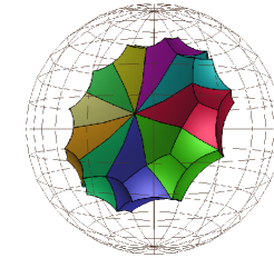
Figure 9: Tiling the Löbell $10$ polyhedron with $10$ copies of the $(4,4,5)$ truncated cube.

The approximate volumes were computed using Damian Heard’s program Orb [11]. (Orb provides twice the volume of the polyhedron, which is the volume of the orbifold obtained by gluing the polyhedron to it’s mirror image along its boundary.)

7.8 Pairs not distinguished by $k\Gamma$ and $A\Gamma$

We found three pairs of non-arithmetic polyhedral reflection groups which are indistinguishable by the invariant trace field and the invariant quaternion algebra. The first of these is the pair of doubly truncated prisms with $q=5$, from Subsection 7.6. Each of these has the same volume, approximately $2.73952694$ since the second can be obtained from the first by cutting in a horizontal plane and applying a $\frac{1}{3}$ twist. We leave it as an open question to the reader whether the two polyhedra in the first pair are commensurable.

The second and third pairs are the $(4,4,5)$ truncated cube and the Löbell $10$ polyhedron and the $(4,4,6)$ truncated cube and the Löbell $12$ polyhedron, each of which fit into the general commensurability between the $(4,4,n)$ truncated cube and the Löbell $2n$ polyhedron, as described in the previous subsection.

Appendix A Computing finite ramification of quaternion algebras

Recall from Section 4 that to determine whether two quaternion algebras over a number field $F$ are isomorphic it suffices to compare their ramification over all real and finite places of $F$.

To compute the finite ramification of a quaternion algebra $A\cong\left(\frac{a,b}{F}\right)$ we first recall that there are a finite number of candidate primes over which $A$ can ramify: $A$ necessarily splits (is unramified) over any prime ideal not dividing the ideal $\langle 2ab\rangle$. To check those primes ${\cal P}$ dividing $\langle 2ab\rangle$, we apply Theorem 4 which states that $A$ splits over ${\cal P}$ if and only if there is a solution to the Hilbert Equation $aX^{2}+bY^{2}=1$ in the completion $F_{\nu}$. Here $\nu$ is the valuation given by $\nu(x)=c^{n_{\cal P}(x)}$ on $R_{F}$, see Section 4.

Because it is difficult to do computer calculations in the completion $F_{\nu}$, where elements are described by infinite sequences of elements of $F$, we ultimately want to reduce our calculations to be entirely within $R_{F}$. Hensel’s Lemma, see [18], is the standard machinery for this reduction. Happily, for the problem at hand, the proper use of Hensel’s Lemma has previously been worked out, see [9] (whose authors write $\nu_{\cal P}$ instead of our $n_{\cal P}$ and $|\cdot|$ instead of our $\nu$). We use the same techniques they do but without many of the optimizations, which we find unnecessary for our program (this is not the bottleneck in our code). The following theorem provides the necessary reduction:

Theorem 16

Let ${\cal P}$ be a prime ideal in $R_{F}$, let $a,b\in R_{F}$ be such that $n_{\cal P}(a),n_{\cal P}(b)\in\{0,1\}$, and define an integer $m$ as follows: if ${\cal P}|2$, $m=2n_{\cal P}(2)+3$ and if ${\cal P}\not|\,2$ then $m=1$ if $n_{\cal P}(a)=n_{\cal P}(b)=0$ and $m=3$ otherwise.

Let $S$ be a finite set of representatives for the ring $R_{F}/{\cal P}^{m}.$ The Hilbert Equation

$$aX^{2}+bY^{2}=1$$

has a solution with $X$ and $Y\in F_{\nu}$ if and only if there exist elements $X^{\prime},Y^{\prime},$ and $Z^{\prime}\in S$ such that

$$\nu(aX^{\prime 2}+bY^{\prime 2}-Z^{\prime 2})\leq c^{m}$$

and $\max\{\nu(X^{\prime}),\nu(Y^{\prime}),\nu(Z^{\prime})\}=1$.

Recall that $0<c<1$ is the arbitrary constant that appears in the definition of $\nu$. Also note that the condition that $n_{\cal P}(a),n_{\cal P}(b)\in\{0,1\}$ is no real restriction since one can always divide the elements of $F$ appearing in the Hilbert symbol by any squares in the field without changing $A$.

Our Theorem 16 is a minor extension of Proposition 4.9 of [9]. Their proposition only applies to dyadic primes, corresponding to $m=2n_{\cal P}(2)+3.$ The other two cases can be proved analogously using, instead of their Lemma 4.8, the following statement:

Lemma 17

Suppose that $\nu$ is the valuation corresponding to a non-dyadic prime ${\cal P}$. Let $X,X^{\prime}$ be in $F_{\nu}$ and suppose that $\nu(X)\leq 1$ and $\nu(X-X^{\prime})\leq c^{k}$ for some non-negative integer $k$. Then, $\nu(X^{2}-X^{\prime 2})\leq c^{2k}$.

The reason we make this minor extension of Proposition 4.9 from [9] is that we do not implement the optimizations for non-dyadic primes that appear in SNAP, instead choosing to use the Hilbert Equation in all cases.

Thus, the problem of determining finite ramification of $A$ reduces to finding solutions in $R_{F}$ to the Hilbert inequality from Theorem 16. Our program closely follows SNAP [10], solving the equation by exploring, in depth-first order [8], a tree whose vertices are quadruples $(X,Y,Z,n)$, where $\nu(aX^{2}+bY^{2}-Z^{2})\leq c^{n}$. The children of the vertex $(X,Y,Z,n)$ are the vertices $(X_{1},Y_{1},Z_{1},n+1)$ where $X_{1}\equiv X,Y_{1}\equiv Y,\mbox{ and }Z_{1}\equiv Z\pmod{{\cal P}^{n}}$. In fact, the condition $\max\{\nu(X),\nu(Y),\nu(Z)\}=1$ means that the search space is considerably reduced because there must be a solution to the inequality with one of $X,Y,Z$ equal to $1$. Indeed, if $\nu(Y)=1$ then $Y$ is invertible modulo any power of ${\cal P}$ and $(XY^{-1},1,ZY^{-1})$ is also a solution. So, our program only searches the three sub-trees given by fixing $X,Y,$ or $Z$ at $1$. In the case that we search all three trees up to level $n=m$ unsuccessfully, then Theorem 16 guarantees that there is no solution to the Hilbert Equation, and consequently $A$ ramifies over ${\cal P}$.

References

- [1] www.geomview.org, Developed by The Geometry Center at the University of Minnesota in the late 1990’s.
- [2] Ian Agol. Finiteness of arithmetic Kleinian reflection groups. In International Congress of Mathematicians. Vol. II, pages 951–960. Eur. Math. Soc., Zürich, 2006.
- [3] E. M. Andreev. On convex polyhedra in Lobacevskii spaces (English Translation). Math. USSR Sbornik, 10:413–440, 1970.
- [4] Omar Antolín-Camarena, Gregory R. Maloney, and Roland K. W. Roeder. SNAP-HEDRON: a computer program for computing arithmetic invariants of polyhedral reflection groups. http://www.math.toronto.edu/~rroeder/SNAP-HEDRON.
- [5] Michel Boileau and Joan Porti. Geometrization of 3-orbifolds of cyclic type. Astérisque, (272):208, 2001. Appendix A by Michael Heusener and Porti.
- [6] Phil Bowers and Kenneth Stephenson. A branched Andreev-Thurston theorem for circle packings of the sphere. Proc. London Math. Soc. (3), 73(1):185–215, 1996.
- [7] Henri Cohen. A course in computational algebraic number theory, volume 138 of Graduate Texts in Mathematics. Springer-Verlag, Berlin, 1993.
- [8] Thomas H. Cormen, Charles E. Leiserson, and Ronald L. Rivest. Introduction to algorithms. The MIT Electrical Engineering and Computer Science Series. MIT Press, Cambridge, MA, 1990.
- [9] David Coulson, Oliver A. Goodman, Craig D. Hodgson, and Walter D. Neumann. Computing arithmetic invariants of 3-manifolds. Experiment. Math., 9(1):127–152, 2000.
- [10] O. A. Goodman, C. D. Hodgson, and Neumann w. D. “snap home page”. See http://www.ms.unimelb.edu.au/~snap. Includes source distribution and extensive tables of results of Snap computations.
- [11] Damian Heard. “Orb”. See http://www.ms.unimelb.edu.au/~snap/orb.html.
- [12] Martin Hildebrand and Jeffrey Weeks. A computer generated census of cusped hyperbolic -manifolds. In Computers and mathematics (Cambridge, MA, 1989), pages 53–59. Springer, New York, 1989.
- [13] Hugh M. Hilden, María Teresa Lozano, and José María Montesinos-Amilibia. On the Borromean orbifolds: geometry and arithmetic. In Topology ’90 (Columbus, OH, 1990), volume 1 of Ohio State Univ. Math. Res. Inst. Publ., pages 133–167. de Gruyter, Berlin, 1992.
- [14] C. D. Hodgson. Deduction of Andreev’s theorem from Rivin’s characterization of convex hyperbolic polyhedra. In Topology 90, pages 185–193. de Gruyter, 1992.
- [15] Craig Hodgson and Jeff Weeks. A census of closed hyperbolic 3-manifolds. ftp://www.geometrygames.org/priv/weeks/SnapPea/SnapPeaCensus/ClosedCens%us/.
- [16] Roland K. W. Roeder John H. Hubbard and William D. Dunbar. Andreev’s theorem on hyperbolic polyhedra. Les Annales de l’Institute Fourier, 57(3):825–882, 2007.
- [17] Taiyo Inoue. Organizing volumes of right angled hyperbolic polyhedra. Doctoral thesis, 2007. University of California, Berkeley.
- [18] Serge Lang. Algebraic number theory, volume 110 of Graduate Texts in Mathematics. Springer-Verlag, New York, second edition, 1994.
- [19] A. K. Lenstra, H. W. Lenstra, Jr., and L. Lovász. Factoring polynomials with rational coefficients. Math. Ann., 261(4):515–534, 1982.
- [20] F. Löbell. Beispiele geschlossener dreidimensionaler clifford-kleinische räume negativer krümmung. Ber. Sächs. Akad. Wiss., 83:168–174, 1931.
- [21] C. Maclachlan and A. W. Reid. Invariant trace-fields and quaternion algebras of polyhedral groups. J. London Math. Soc. (2), 58(3):709–722, 1998.
- [22] Colin Maclachlan and Alan W. Reid. The arithmetic of hyperbolic 3-manifolds, volume 219 of Graduate Texts in Mathematics. Springer-Verlag, New York, 2003.
- [23] Walter D. Neumann and Alan W. Reid. Arithmetic of hyperbolic manifolds. In Topology ’90 (Columbus, OH, 1990), volume 1 of Ohio State Univ. Math. Res. Inst. Publ., pages 273–310. de Gruyter, Berlin, 1992.
- [24] I. Rivin and C. D. Hodgson. A characterization of compact convex polyhedra in hyperbolic 3-space. Invent. Math., 111:77–111, 1993.
- [25] Roland K. W. Roeder. Constructing hyperbolic polyhedra using newton’s method. To appear, Experimental Mathematics. See also arXiv:math/0603552.
- [26] Kisao Takeuchi. Arithmetic triangle groups. J. Math. Soc. Japan, 29(1):91–106, 1977.
- [27] The PARI Group, Bordeaux. PARI/GP, version 2.1.7, 2005. available from http://pari.math.u-bordeaux.fr/.
- [28] A. Yu. Vesnin. Personal communication.
- [29] A. Yu. Vesnin. Three-dimensional hyperbolic manifolds with a common fundamental polyhedron (translation). Math. Notes, 49(5-6):575–577, 1991.
- [30] Andrei Vesnin. Three-dimensional hyperbolic manifolds of löbell type. Siberian Math. J, 28(5):731–733, 1987.
- [31] Marie-France Vignéras. Arithmétique des algèbres de quaternions, volume 800 of Lecture Notes in Mathematics. Springer, Berlin, 1980.
- [32] È. B. Vinberg. Discrete groups generated by reflections in Lobačevskiĭ spaces. Mat. Sb. (N.S.), 72 (114):471–488; correction, ibid. 73 (115) (1967), 303, 1967.
- [33] È. B. Vinberg and O. V. Shvartsman. Discrete groups of motions of spaces of constant curvature. In Geometry, II, volume 29 of Encyclopaedia Math. Sci., pages 139–248. Springer, Berlin, 1993.