MORPHOLOGICAL EFFECTS ON SURFACE PLASMON POLARITONS AT THE PLANAR INTERFACE OF A METAL AND A COLUMNAR THIN FILM

John A. Polo Jr¹ and Akhlesh Lakhtakia^2
1Department of Physics and Technology,
Edinboro University of Pennsylvania,
Edinboro, PA 16444, USA.
e–mail: polo@edinboro.edu
fax: (814) 732-2455
²CATMAS — Computational & Theoretical Materials Sciences Group,
Department of Engineering Science and Mechanics,
Pennsylvania State University,
University Park, PA 16802, USA.
e–mail: akhlesh@psu.edu

ABSTRACT Surface plasmon polaritons (SPPs) at the interface of a columnar thin film (CTF) and metal exist over a range of propagation directions relative to the morphology of the CTF which depends on the tilt of the columns in the CTF. The phase speed of the SPP wave varies mainly as a function of the tilt of the CTF columns. Both the confinement of the SPP wave to the interface and the decay of the SPP wave along the direction of propagation depend strongly on the direction of propagation relative to the morphologically significant plane of the CTF. The greater the columnar tilt in relation to the interface, the shorter is the range of propagation. Because of its porosity and the ability to engineer this biaxial dielectric material, the CTF–metal interface may be more attractive than traditional methods of producing SPPs.

Keywords: surface plasmon polariton, columnar thin film, titanium oxide

1. INTRODUCTION

The surface plasmon polariton (SPP) has been the object of intense investigation for several decades [1]. In recent years, the understanding of the phenomenon has been harnessed for a wide array of analytical and biomedical applications [2, 3, 4]. Although various configurations are used to launch and detect the SPP, in the Kretschmann configuration, a metal film is interposed between a low-refractive-index dielectric medium and a high-refractive-index dielectric medium [5]. A light beam is launched in the high-refractive-index medium to impinge on the planar interface between that medium and the metal. The SPP travels along the planar interface of the metal and the low-refractive-index medium.

The propagation of SPPs at the planar interface of a metal and an anisotropic dielectric material has been examined theoretically [6]. For this communication, we investigated the propagation of the SPP along the interface of a metal and a columnar thin film (CTF), in relation to the morphology of the CTF. The columnar thin film, an artificial material, is effectively an optically biaxial continuum [7], and porous [8, Ch. 6]. The porous CTF may offer a medium in which to embed analyte and/or recognition molecules to which the analyte may bind.

A columnar thin film is produced by directing a vapor at an angle $\chi_{v}$ to a substrate. Under suitable conditions, parallel columns form at an angle $\chi\geq\chi_{v}$ to the substrate; see Figure 1. The columns are composed of multimolecular clusters with $\sim 3$ nm diameter which, in turn, form columns with $\sim 100$ nm cross–sectional diameter, depending on the evaporant species and the deposition conditions. The geometry considered here is the same as that in a predecessor paper [9], except that the substrate is now made of a metal instead of a transparent dielectric, and is also illustrated in Figure 1.

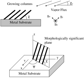
Figure 1: Geometry of CTF–metal interface and SPP–wave propagation.

The plan of the communication is as follows. Section 2 contains a description of the geometry of the problem and the constitutive relations. For the details of the field representation and the derivation of the dispersion relation for the SPP wave, we refer the reader to the predecessor paper [9]. Numerical results for a particular CTF–metal interface, titanium oxide CTF–aluminum, are presented in Section 3. Concluding remarks are presented in Section 4.

The following assumption and notational conventions are used. An $\exp(-i\omega t)$ time–dependence is implicit, with $\omega$ denoting the angular frequency. The free–space wavenumber, the free–space wavelength, and the intrinsic impedance of free space are denoted by $k_{o}=\omega\sqrt{\epsilon_{o}\mu_{o}}=\omega/c_{o}$, $\lambda_{o}=2\pi/k_{o}$, and $\eta_{o}=\sqrt{\mu_{o}/\epsilon_{o}}$, respectively, with $\mu_{o}$ and $\epsilon_{o}$ being the permeability and permittivity of free space. Vectors are underlined, and dyadics are underlined twice. Cartesian unit vectors are identified as ${\underline{u}}_{x}$, ${\underline{u}}_{y}$ and ${\underline{u}}_{z}$.

2. GEOMETRY AND CONSTITUTIVE RELATIONS

The geometry of the problem is illustrated in Figure 1. With the interface between the metal substrate and the CTF denoted by $z=0$, the metal occupies the half–space $z<0$, while the CTF occupies the half–space $z>0$. Without loss of generality, the direction of propagation is taken to be parallel to the $x$–axis, and the angle between the direction of propagation and the morphologically significant plane [8, Ch. 7] of the the CTF is denoted by $\psi$ .

The relative permittivity dyadic of the CTF may be stated as [8, Ch. 7]

$$\underline{\underline{\epsilon}}_{CTF}=\left(n_{a}^{2}\,{\underline{u}}_{n}{\underline{u}}_{n}+n_{b}^{2}\,{\underline{u}}_{\tau}{\underline{u}}_{\tau}+n_{c}^{2}\,{\underline{u}}_{b}{\underline{u}}_{b}\right)\,,$$ (1)

where $n_{a,b,c}$ are the principal refractive indexes and the unit vectors

$$\left.\begin{array}[]{l}{\underline{u}}_{n}=-({\underline{u}}_{x}\cos\psi+{\underline{u}}_{y}\sin\psi)\sin\chi+{\underline{u}}_{z}\cos\chi\\ {\underline{u}}_{\tau}=({\underline{u}}_{x}\cos\psi+{\underline{u}}_{y}\sin\psi)\cos\chi+{\underline{u}}_{z}\sin\chi\\ {\underline{u}}_{b}=-{\underline{u}}_{y}\cos\psi+{\underline{u}}_{x}\sin\psi\end{array}\right\}\,.$$ (2)

All four quantities — $n_{a,b,c}$ and the column inclination angle $\chi$ — depend on the evaporant species and the vapor incidence angle $\chi_{v}$. The refractive index of the metal is denoted by $n_{s}$.

Expressions for the field equations and dispersion relation have been worked out elsewhere [9]. It suffices to mention that the wave vector in the substrate may be written as

$${\underline{k}}_{s}=k_{o}\,(\varkappa\,{\underline{u}}_{x}-iq_{s}\,{\underline{u}}_{z})\,,$$ (3)

where $\varkappa$ and

$$q_{s}=+\sqrt{\varkappa^{2}-n_{m}^{2}}\,$$ (4)

are the normalized propagation constant and the decay constant, respectively. In order for the SPP wave to be confined to the interface $z=0$, we must have ${\rm Re}\left[q_{s}\right]>0$. Unlike for the CTF–dielectric interface [9], $\varkappa$ is expected to be complex valued since the dissipative properties of the metal can not be ignored. Similarly, in the half–space $z>0$ occupied by the CTF, the wavevector may be written as

$${\underline{k}}_{c}=k_{o}\,(\varkappa\,{\underline{u}}_{x}+iq_{c}\,{\underline{u}}_{z})\,,$$ (5)

and again we must have ${\rm Re}\left[q_{c}\right]>0$ for localization of the SPP wave to the interface. The SPP wave comprises two partial waves in the CTF, identified by $q_{c1}$ and $q_{c2}$.

3. NUMERICAL RESULTS

Hodgkinson et al. [10] measured the constitutive relations for CTFs made of oxides of tantalum, titanium, and zirconium. We chose titanium oxide to illustrate SPP propagation at a planar CTF–metal interface. The empirical relationships determined at $\lambda_{o}=633$ nm for the titanium–oxide CTF can be written as

$$n_{a} = 1.0443+2.7394\left(\frac{\chi_{v}}{\pi/2}\right)-1.3697\left(\frac{\chi_{v}}{\pi/2}\right)^{2}\,,$$ (6)

$$n_{b} = 1.6765+1.5649\left(\frac{\chi_{v}}{\pi/2}\right)-0.7825\left(\frac{\chi_{v}}{\pi/2}\right)^{2}\,,$$ (7)

$$n_{c} = 1.3586+2.1109\left(\frac{\chi_{v}}{\pi/2}\right)-1.0554\left(\frac{\chi_{v}}{\pi/2}\right)^{2}\,,$$ (8)

and

$$\tan\chi = 2.8818\tan\chi_{v}\,,$$ (9)

where $\chi_{v}$ and $\chi$ are in radian. We must caution that the foregoing expressions are applicable to CTFs produced by one particular experimental apparatus, but may have to be modified for CTFs produced by other researchers on different apparatuses; hence, we used these expressions for the numerical results presented in this section merely for illustration. Metals commonly used for SPP systems are aluminum, copper, silver, and gold. For illustration, we chose aluminum with a complex refractive index $n_{s}=1.38+7.61i$ at $\lambda_{o}=633$ nm [11]. We note that values of $\varkappa$ for SPP propagation when $\psi=0^{\circ}$ have been reported elsewhere [12].

Calculations were carried out for $\chi_{v}=7.2^{\circ},20^{\circ},60^{\circ}$, and $90^{\circ}$. The lowest value $\chi_{v}=7.2^{\circ}$ corresponds to $\chi=20^{\circ}$ and represents the approximate, currently achievable lower limit of $\chi$. As previously stated, the wave number $\kappa=k_{o}\varkappa$ along the direction of propagation must be complex valued. The real part of $\kappa$ determines the phase speed $v=\omega/{\rm Re}(\kappa)$ of the SPP wave. The phase speed relative to the speed of light in vacuum is calculated as

$$v_{rel}=\frac{v}{c_{o}}=\frac{1}{{\rm Re}(\varkappa)}\,.$$ (10)

Figure 2 shows $v_{rel}$ as a function of $\psi$ for $\chi_{v}=7.2^{\circ},20^{\circ},60^{\circ}$, and $90^{\circ}$, with $\psi$ restricted to the range $[0^{\circ},90^{\circ}]$.

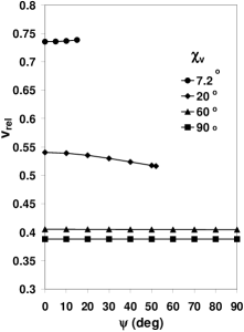
Figure 2: Phase speed of the SPP wave at the planar interface of a titanium–oxide CTF and an aluminum substrate, relative to the speed of light in vacuum, versus $\psi$ for $\chi_{v}=7.2^{\circ}$, $20^{\circ}$, $60^{\circ}$, and $90^{\circ}$.

The curves are drawn over the $\psi$–ranges for which the boundary conditions at $z=0$ could be satisfied and thus represent the ranges over which a SPP wave can exist. For each value of $\psi$ shown, at which a SPP wave exists, there also exist three other values at $-\psi$, $180^{\circ}+\psi$, and $180^{\circ}-\psi$ with an identical value of $v_{rel}$. The relative phase speed $v_{rel}$ decreases as $\chi_{v}$ increases with the most rapid change occurring at the low end of the $\chi_{v}$–range.

The greatest variation of $v_{rel}$ as a function of $\psi$ is observed for $\chi_{v}=20^{\circ}$. This curve has a downward slope as $v_{rel}$ decreases from roughly 0.540 to 0.516 as $\psi$ changes from $0^{\circ}$ to $52^{\circ}$. At $\chi_{v}=60^{\circ}$, a much smaller change is observed: $v_{rel}$ decreases from roughly 0.4050 to 0.4045 as $\psi$ changes from $0^{\circ}$ to $90^{\circ}$. In contrast, the curve for $\chi_{v}=7.2^{\circ}$ shows an upward slope as $v_{rel}$ changes from roughly 0.735 to 0.738 as $\psi$ varies from $0^{\circ}$ to $15^{\circ}$. Of course, the curve for $\chi_{v}=90^{\circ}$ is completely flat as required by symmetry since Eqs. (6)–(9) predict that the generally biaxial CTF becomes uniaxial at $\chi_{v}=90^{\circ}$ with the axis of symmetry perpendicular to the interface $z=0$.

The imaginary part of $\kappa$ determines the rate at which the SPP wave decays along the direction of propagation. The e–folding distance for decay of the wave amplitude relative to the wavelength $\lambda_{o}$ may be calculated as

$$\overline{x}_{ef}=\frac{1}{2\pi\,{\rm Im}(\varkappa)}\,.$$ (11)

Figure 3 shows $\overline{x}_{ef}$ as a function of $\psi$ over the restricted range $[0^{\circ},90^{\circ}]$. As with $v_{rel}$, for each value of $\psi$ displayed, an identical value of $\overline{x}_{ef}$ is obtained at $-\psi$, $180^{\circ}+\psi$, and $180^{\circ}-\psi$. As $\chi_{v}$ increases, $\overline{x}_{ef}$ decreases and the curve of $\overline{x}_{ef}$ vs. $\psi$ flattens. At $\chi_{v}=60^{\circ}$, the curve is nearly flat with only $\sim 2\%$ change over the entire $\psi$–range. In contrast, at $\chi_{v}=7.2^{\circ}$ and $20^{\circ}$, $\overline{x}_{ef}$ changes by nearly two orders of magnitude.

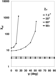
Figure 3: e–folding distance of the SPP wave along the $x$–direction, the direction of propagation, versus $\psi$ for the same conditions as in Figure 2.

Figures 2 and 3 let us conclude that an increase in the vapor incidence angle (i) reduces the phase speed and (ii) increases the attenuation of the SPP wave. Thus, a high value of $\chi_{v}$ is inimical to long–range propagation for all $\psi$, an understanding previous obtained only for the case of the direction of propagation lying in the morphologically significant plane (i.e., $\psi=0^{\circ}$) [12]. The properties of the SPP wave along the $z$–axis, perpendicular to the direction of propagation, are described by

• $q_{c1}$ and (ii) $q_{c2}$ for the two partial waves in the CTF, and

• $q_{m}$ in the metal.

Similar to $\overline{x}_{ef}$, three e–folding distances in the $z$–direction relative to the wavelength in vacuum may be calculated as

$$\left.\begin{array}[]{lll}\overline{z}_{ef1}&=&\frac{1}{2\pi\,{\rm Im}(q_{c1})}\\[5.0pt] \overline{z}_{ef2}&=&\frac{1}{2\pi\,{\rm Im}(q_{c2})}\\[5.0pt] \overline{z}_{efm}&=&\frac{1}{2\pi\,{\rm Im}(q_{m})}\end{array}\right\}\,.$$ (12)

Figure 4 shows these three quantities as functions of $\psi$ over the restricted range $[0^{\circ},90^{\circ}]$. These three quantities describe the localization of the SPP wave to the interface. In Figure 4a, the curves of $\overline{z}_{ef1}$ are similar to those of $\overline{x}_{ef}$ displayed in Figure 3, with the curves for both $\chi_{v}=60^{\circ}$ and $90^{\circ}$ essentially flat. At $\chi_{v}=7.2^{\circ}$ and $20^{\circ}$, $\overline{z}_{ef1}$ varies by about two orders of magnitude. Thus, for the two values of $\chi_{v}$ for which the $\psi$–range for surface wave propagation ends and does not continue to $\psi\geq 90^{\circ}$, the first partial–wave component of the SPP wave in the CTF becomes delocalized as $\psi$ approaches the end of its range.

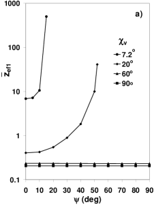
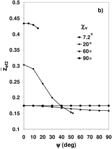
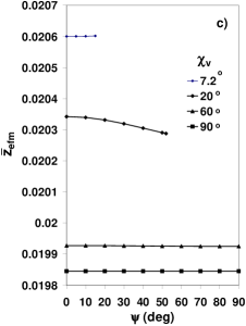
Figure 4: e–folding distances of the SPP wave relative to $\lambda_{o}$ in the $z$–direction for the same conditions as in Figure 2: a) partial wave 1 in CTF; b) partial wave 2 in CTF; c) in aluminum.

In Figure 4b, the curves of $\overline{z}_{ef2}$ versus $\psi$ are also nearly flat for both $\chi_{v}=60^{\circ}$ and $90^{\circ}$. At $\chi_{v}=7.2^{\circ}$ and $20^{\circ}$, $\overline{z}_{ef2}$ decreases as $\psi$ increases. The second partial–wave component, then, becomes more localized as $\psi$ approaches the end of its range.

The e–folding distance in the metal, $\overline{z}_{efm}$, is essentially flat for all values of $\chi_{v}$ in Figure 4c. The greatest variation of $\overline{z}_{efm}$ occurs when $\chi_{v}=20^{\circ}$, but is still less than 0.4%.

Unlike $v_{rel}$ and $\overline{x}_{ef}$, the values of the e–folding distances in the $z$–direction for the CTF are not identical at $\psi$, $-\psi$, $180^{\circ}+\psi$, and $180^{\circ}-\psi$. The value of any e–folding distance in the $z$–direction at $\psi$ is, however, equal to the value at $-\psi$, and the value at $180^{\circ}+\psi$ is equal to that at $180^{\circ}-\psi$. Since the difference in most cases is slight, we present the percent difference between the values at $\psi$ and $-\psi$, and the values at $180^{\circ}+\psi$ and $180^{\circ}-\psi$ in Figure 5. The % differences for the e–folding distance of the first partial–wave component in the CTF, $\overline{z}_{ef1}$, are shown in Figure 5a. The curve for $\chi_{v}=7.2^{\circ}$ shows the largest difference of about 13% and occurs at the end of the $\psi$–range where $\psi=15^{\circ}$. The difference decreases rapidly with increasing $\chi_{v}$. At $\chi_{v}=60^{\circ}$, the maximum difference is only about 0.1%. Differences in e–folding distances for the partial–wave component 2 in the CTF are shown in Figure 5b with the maximum observed value of 1.5% —  almost an order of magnitude smaller than for the partial–wave component 1. Differences in e–folding distances appear to decrease as $\chi_{v}$ increases with a maximum difference at $\chi_{v}=60^{\circ}$ of only about 0.01%. However, the decrease is not monotonic as the maximum difference at $\chi_{v}=20^{\circ}$ is about 50% larger than that at $\chi_{v}=7.2^{\circ}$.

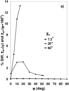
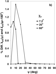
Figure 5: The % difference between $\overline{z}_{ef1}(\psi)$ and $\overline{z}_{ef2}(180^{\circ}+\psi)$ for same conditions as in Figure 2.

4. CONCLUSION

Examining SPP–wave propagation at a planar CTF–metal interface, with demonstrated empirical data to characterize both the CTF and the metal, we found that the direction, denoted by $\psi$, at which SPP–wave propagation is possible is limited, in general, and depends on the tilt angle $\chi$ of the columns in the CTF. This tilt angle may be predicted from the vapor incidence angle $\chi_{v}$ set during the manufacture of the film. The $\psi$–range for SPP waves increases as $\chi_{v}$ increases. At sufficiently large values of $\chi_{v}$, SPP propagation becomes possible in all directions. Even at the lowest value $(\chi_{v}=7.2^{\circ}$) examined by us, the $\psi$–range is greater than $10^{\circ}$. This is in contrast to surface–wave propagation at the interface of a CTF and an isotropic dielectric material, for which the $\psi$–range is only a fraction of a degree for all values of $\chi$ [9].

The phase speed of the SPP wave shows a strong dependence on $\chi_{v}$, but is also mildly dependent on $\psi$. The e–folding distance along the direction of propagation is strongly dependent on $\psi$ at low values of $\chi_{v}$, varying by several orders of magnitude, but is relatively flat at larger values of $\chi_{v}$. A high value of $\chi_{v}$ is inimical to long–range propagation for all $\psi$. At the end of the $\psi$–range, for those values of $\chi_{v}$ for which the propagation directions are limited, the SPP wave becomes delocalized from the interface on the CTF side. This is seen as an apparent divergence in the e–folding distance in the direction perpendicular to the interface for one of the two partial waves in the CTF as $\psi$ approaches the end of its range. The e–folding distance perpendicular to the interface for the other partial wave in the CTF, on the other hand, tends to decrease as $\psi$ approaches its limiting value. In the metal, the e–folding distance perpendicular to the interface does not vary much with $\psi$.

The demonstration of a SPP wave at the interface of a CTF and a metal offers certain options in SPP technology. With a wide choice of possible evaporant materials [13] and vapor incidence angles, the CTF–metal interface offers a large latitude in the engineering of SPP systems. The porosity of the CTFs may also offer some advantages. With its nano–scale porous structure, a CTF could allow molecular–scale analytes to reach the interface for analysis while screening out larger particulates. The detection of viruses has become important in recent times. CTFs with pores on the nano–scale may allow viruses access to the interface while excluding larger organisms. Through photolithographic techniques it is possible to pattern CTFs [14]. Various samples could be placed, possibly in the field, on isolated CTF patches on a single substrate for later analysis. Also, different patches could be embedded with different recognition molecules which could be used to perform multiple searches on a single sample. Other options have yet to be imagined.

References

- [1] J. M. Pitarke, V. M. Silkin, E. V. Chulkov, and P. M. Echenique, Theory of surface plasmons and surface-plasmon polaritons, Rep. Prog. Phys. 70 (2007), 1-87.
- [2] J. Homola, S. S. Yee, G. Gauglitz, Surface plasmon resonance sensors: review, Sens. Actuat. B: Chem. 54 (1999), 3-15.
- [3] J. Homola, Present and future of surface plasmon resonance biosensors, Anal. Bioanal. Chem. 377, 528-539 (2003).
- [4] S. K. Arya, A. Chaubey, and B. D. Malhotra, Fundamentals and applications of biosensors, Proc. Indian Natn. Sci. Acad. 72 (2006), 249-266.
- [5] E. Kretschmann and H. Raether, Radiative decay of nonradiative surface plasmons excited by light, Zeit. Naturforsch. A 23 (1968), 2135-2136.
- [6] V. M. Agranovich and D. L. Mills (eds.), Surface polaritons: Electromagnetic waves at surfaces and interfaces, North-Holland, Amsterdam, 1982.
- [7] I. J. Hodgkinson and Q. h. Wu, Birefringent thin films and polarizing elements, World Scientific, Singapore, 1997.
- [8] A. Lakhtakia and R. Messier, Sculptured thin films: Nanoengineered morphology and optics, SPIE Press, Bellingham, WA, 2005.
- [9] J. A. Polo, Jr., S. R. Nelatury, and A. Lakhtakia, Propagation of surface waves at the planar interface of a columnar thin film and an isotropic substrate, J. Nanophoton. 1 (2007), 013501.
- [10] I. J. Hodgkinson, Q. h. Wu, and J. Hazel, Empirical equations for the principal refractive indices and column angle of obliquely deposited films of tantalum oxide, titanium oxide, and zirconium oxide, Appl. Opt. 37 (1998), 2653-2659.
- [11] M. Mansuripur and L. Li, What in the world are surface plasmons?, OSA Opt. Photon. News, 8 (1997) 50-55 (May issue).
- [12] A. Lakhtakia and J. A. Polo, Jr., Morphological influence on surface–wave propagation at the planar interface of a metal film and a columnar thin film, Asian J. Phys. (accepted for publication, 2007); also: arXiv:0706.4306.
- [13] H. A. Macleod, Thin–film optical filters, 3rd ed., CRC Press, Boca Raton, FL, 2001.
- [14] M. W. Horn, M. D. Pickett, R. Messier, and A. Lakhtakia, Blending of nanoscale and microscale in uniform large–area sculpured thin–film architectures, Nanotechnology 15 (2004), 303-310.