Beaming Binaries — a New Observational Category of Photometric Binary Stars

Abstract

The new photometric space-borne survey missions CoRoT and Kepler will be able to detect minute flux variations in binary stars due to relativistic beaming caused by the line-of-sight motion of their components. In all but very short period binaries ($P>10$ d), these variations will dominate over the ellipsoidal and reflection periodic variability. Thus, CoRoT and Kepler will discover a new observational class: photometric beaming binary stars. We examine this new category and the information that the photometric variations can provide. The variations that result from the observatory heliocentric velocity can be used to extract some spectral information even for single stars.

1 Introduction

In 2003 Loeb & Gaudi suggested a new photometric method to detect extrasolar planets, based on the minute variability of the stellar flux due to relativistic beaming induced by the star’s reflex radial velocity. Rybicki & Lightman (1979) show that several factors contribute to the beaming effect. The bolometric factors are the Lorentz transformations of the radiated energy and the time intervals, and the modification of the angular distribution of the radiated energy (stellar aberration). Thus, in the limit where the star’s radial (line-of-sight) velocity $v_{\mbox{\tiny R}}$ is much smaller than the speed of light $c$, the observed bolometric flux $F$ is modified relative to the emitted bolometric flux $F_{0}$ as

$$F=F_{0}\left(1+4\frac{v_{\mbox{\tiny R}}}{c}\right)\ .$$ (1)

For band-pass photometry, the Doppler shift of the emitted frequency and the spectral index of the source spectrum also have to be taken into account, which finally yields:

$$F_{\nu}=F_{\nu\mbox{\tiny 0}}\left[1+(3-\alpha)\frac{v_{\mbox{\tiny R}}}{c}\right]\ ,$$ (2)

where $F_{\nu}$ and $F_{\nu\mbox{\tiny 0}}$ are the observed and emitted flux density at frequency $\nu$, respectively, and $\alpha=d\log F/d\log\nu$ is the average spectral index around the observed frequency. Note that Equations 1 and 2 can also be obtained in a semi-classical context. In any case, since the effect depends on the first order of $v_{\mbox{\tiny R}}/c$ the velocities do not need to be highly relativistic to detect the effect. Detecting beaming variability related to orbital motion requires the very high precision provided by photometric satellites. Even in the extremely high orbital velocities of the stars orbiting the massive black hole in the Galactic Center, the beaming effects cannot be measured with the low photometric precision available for those stars (Zucker et al., 2006).

Loeb & Gaudi (2003) suggested to detect stellar periodic motion induced by an unseen planet through the beaming effect. They showed that the amplitude of the beaming effect produced by an extrasolar planet is of the order of micro-magnitude. Such an effect is barely detectable by the new photometric space missions CoRoT (Baglin, 2003) and Kepler (Basri, Borucki & Koch, 2005), which are aiming to find extrasolar transiting planets, with a typical variability amplitude of $100\,\mu$mag. The obvious advantage of Loeb & Gaudi (2003) approach is its applicability to planets with almost any inclination, whereas detecting transiting planets is limited only to planets with orbital inclinations close to $90\arcdeg$.

Here we examine the beaming effect in binary stars, and suggest a new class of binaries — beaming binaries. These are a hybrid between spectroscopic and ellipsoidal binaries, since the beaming binaries will be detected by periodic photometric variations due to their orbital radial velocity. We show that a binary with an orbital period of $P=100\,$d has a beaming variability of at least ${\cal O}(100\,\mu{\mathrm{m}ag})$, which is easily detectable by CoRoT and even more so by Kepler. We further show that for binaries with periods longer than $10$ days, beaming variability dominates over the competing effects of ellipsoidal and reflection variability. We therefore expect the new satellites to harvest hundreds of previously unknown binaries of this new class.

Beaming variability of order $100\,\mu$mag will also be induced by the Earth’s heliocentric motion relative to any observed source, single star or binary. In spectroscopic observations, the effect of the Earth motion is corrected in order to obtain heliocentric radial velocities. Here we show how the dependence of this small variability on the spectral slope at the observed bandpass can be used to probe the spectral characteristics of single and binary stars.

2 The amplitude of the beaming effect as compared with the ellipsoidal and reflection effects

The three kinds of periodic flux variations we expect to detect in binary stars are those due to the ellipsoidal tidal deformations of the stars, the reflection of the light of each star by its companion, and relativistic beaming, which is the subject of this work. Loeb & Gaudi (2003) have presented a rough comparison of those three effects in the context of planet-hosting stars. We now compare the three effects for binary stars, assuming for simplicity a circular ($e=0$) edge-on ($\sin i=90\arcdeg$) orbit. Note that for systems with two stellar components, the observed ellipsoidal effect is the weighted average of the ellipsoidal effects of the two stars, whereas the observed beaming effect is the weighted difference between the beaming variabilities of the two stars, as their effects are exactly in opposite phase. In this respect beaming is similar to the reflection effect.

To a good approximation (see below), the magnitude of the beaming effect can be calculated under the assumption that the two stars radiate as blackbodies. For a blackbody source of temperature $T_{\mathrm{eff}}$ the spectral index $\alpha$ is:

$$\alpha(\nu)=3-\frac{e^{x}}{e^{x}-1}x\ ,$$ (3)

where $x=h\nu/kT_{\mathrm{eff}}$.

The binary’s orbital separation is given by Kepler’s third law,

$$a=\left(\frac{M_{1}+M_{2}}{M_{\sun}}\right)^{1/3}\left(\frac{P}{1\,\mathrm{year}}\right)^{2/3}\,\mathrm{AU}\ ,$$ (4)

where $M_{i}$ are the two masses, with the subscript 1 referring to the primary and 2 to the secondary. The amplitude of the primary’s radial-velocity variation is then

$$K_{1}=\left(\frac{M_{2}}{M_{1}+M_{2}}\right)\left(\frac{a}{1\,\mathrm{AU}}\right)^{-1/2}29.8\,\mathrm{km\,s}^{-1}\ .$$ (5)

A corresponding expression is obtained for the secondary by interchanging the subscripts $1$ and $2$. The peak-to-peak amplitude of the total expected relative flux variation from the binary due to beaming is then

$$\left(\frac{\Delta F_{\nu}}{F_{\nu}}\right)_{\mathrm{beaming}}=\frac{1}{c}\frac{K_{1}[3-\alpha_{1}(\nu)]F_{\nu,\mbox{\tiny 1}}-K_{2}[3-\alpha_{2}(\nu)]F_{\nu,\mbox{\tiny 2}}}{F_{\nu,\mbox{\tiny 1}}+F_{\nu,\mbox{\tiny 2}}}\ .$$ (6)

Note that because the observed effect is the difference between the effects of the two stars, the beaming effect vanishes for an equal-mass binary, where the spectral characteristics are also identical for the two components.

In order to estimate the ellipsoidal variability, we use the expression presented by Morris & Naftilan (1993) for the peak-to-peak ellipsoidal variability of the primary:

$$\left(\frac{\Delta F_{\nu,\mbox{\tiny 1}}}{F_{\nu,\mbox{\tiny 1}}}\right)_{\mathrm{ellips}}\simeq 0.3\frac{(15+u_{1})(1+\tau_{1})}{3-u_{1}}\frac{M_{2}}{M_{1}}\left(\frac{R_{1}}{a}\right)^{3}$$ (7)

Here $\tau_{1}$ is the gravity darkening coefficient of the primary and $u_{1}$ is its limb-darkening coefficient. We calculate a similar expression for the secondary and then weight them by the expected blackbody fluxes in order to obtain the total relative variation of the binary.

Morris & Naftilan (1993) also provide a prescription for calculating the amplitude of the reflection effect. They assume that each star absorbs some of the bolometric flux of its companion, which heats the stellar hemisphere facing the companion, inducing an asymmetric increased emission. Assuming blackbody radiation law, Morris & Naftilan define a ‘luminous-efficiency’ factor by:

$$f_{\lambda}=\left(\frac{T_{2}}{T_{1}}\right)^{4}\frac{e^{x_{2}}-1}{e^{x_{1}}-1}\ ,$$ (8)

where $T_{1}$ and $T_{2}$ are the temperatures of the two components. Like the beaming effect, the contributions of the reflection effects of the two stars are in opposite phase, and the total magnitude of the effect is the weighted difference of the two. Keeping only the leading order terms in the radii (expressed in terms of the orbital separation), we obtain:

$$\left(\frac{\Delta F_{\nu}}{F_{\nu}}\right)_{\mathrm{reflect}}=\frac{2}{3}\frac{\left(R_{2}/a\right)^{2}f_{\lambda}^{-1}F_{\nu,\mbox{\tiny 1}}-\left(R_{1}/a\right)^{2}f_{\lambda}F_{\nu,\mbox{\tiny 2}}}{F_{\nu,\mbox{\tiny 1}}+F_{\nu,\mbox{\tiny 2}}}$$ (9)

Note that the ellipsoidal and reflection variabilities were calculated assuming tidal locking and a circular orbit. Furthermore, we use only the leading order terms in the fractional radii. Thus, we might be overestimating the amplitude of those effects. However, these expressions suffice as conservative estimates for comparing with the beaming effects.

We use Equations 6, 7,and 9 to compare the three effects for three typical binaries and for a range of periods. Table Beaming Binaries — a New Observational Category of Photometric Binary Stars presents the parameters assumed for the stellar components. For the purpose of this simple comparison, we assume $u_{1},u_{2}=0.6$ for our hypothetical stars. We calculate the gravity darkening coefficients using the prescription in Morris (1985).

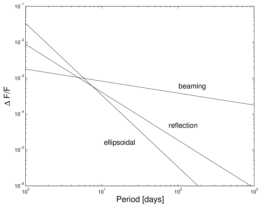
Figure 1: The three periodic photometric effects for an F0-K0 binary star in a range of periods.

Table 2 compares the three effects for the three binaries, observed in the $V$ band, for periods of $10$ and $100$ days. In all cases the beaming variability dominates over the other two effects. Figure 1 shows the three effects for an F0-K0 binary for a range of periods. The corresponding plots for the other cases were very similar. The dependence of the effects on the orbital separation is explicit in the expressions above, and we can use it to understand the dependence on the orbital period. While ellipsoidal variability decreases with period as $P^{-2}$, and the reflection variability as $P^{-4/3}$, the beaming variability only decreases as $P^{-1/3}$, and we expect it to become dominant for long enough periods.

In the three cases we examined the ellipsoidal variability dominates for periods shorter than $8$ days, while for periods longer than $10$ days the beaming variability becomes dominant. Remarkably, the three lines intersect at about the same period, and the reflection effect is almost never dominant. Furthermore, the amplitude of the beaming variability stays at the detectable levels for CoRoT and Kepler, of $0.1-1$ mmag for periods of a hundred days and more.

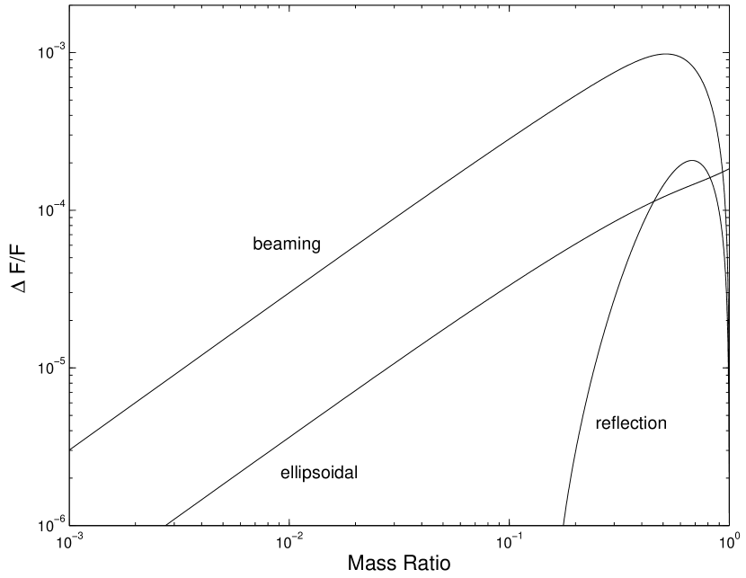
Figure 2: The three periodic photometric effects for a G0 primary in a range of mass ratios.

In Figure 2 we compare the three effects for a range of mass ratios. We assumed a G0 primary, and used power laws for the dependence of the secondary radius and temperature on its mass: $R\propto M^{0.8}$ and $T_{\mathrm{eff}}\propto M^{0.55}$. While the ellipsoidal variability is mostly sensitive to the highest mass ratios, the beaming and reflection effects are more sensitive to intermediary mass ratios. This is mainly because at the highest mass ratios the effects from both binary components are canceled out.

3 Discussion

The radial-velocity beaming lightcurve can yield directly most of the spectroscopic orbital elements, including the period, eccentricity and time of periastron passage. Since these will be obtained as the result of a well defined magnitude-limited photometric survey, they will provide large amounts of new data to statistical studies of spectroscopic binaries, including, e.g., the distribution of orbital period (Duqennoy & Mayor, 1991; Mazeh, Tamuz & North, 2006), and the relation between orbital period and eccentricity (Halbwachs et al., 2003).

The only spectroscopic element that cannot be obtained directly from the lightcurve is the radial-velocity amplitude $K_{1}$. However, as outlined in Equation 6, the $K_{1}$ value can be derived from the amplitude of the beaming effect through the spectral index $\alpha$ of the primary and the relative amplitudes of the beaming effect of the two components of the binary. In most binaries, the secondary is faint enough that we will be able to ascribe the observed beaming variability solely to the primary component. If the primary spectral type is known, we can derive its spectral index ($\alpha$) and obtain $K_{1}$, thus deriving the full set of orbital elements of a single-lined spectroscopic binary.

In order to estimate $\alpha$ and calibrate the relation between the beaming amplitude and $K_{1}$, some spectroscopic follow-up observations of the detected binaries should be performed. Since most of the radial-velocity elements will already be known from photometry, only a small number of observations is needed per star. Multi-object spectrographs, such as FLAMES on the Very Large Telescope (Pasquini et al., 2002) or Hydra on the Wiyn telescope (Barden & Armandroff, 1995), seem like an efficient means to obtain these observations for the detected beaming binaries in the field.

In the few cases where the two components might have very similar magnitudes and masses, the two contributions to the beaming variability may cancel out, because of their opposite phases. In cases where the secondary light will be significant but will not cancel the primary light completely, we will need a photometric analogue of spectroscopic disentangling procedures like TODCOR (Zucker & Mazeh, 1994). Measurements in more than one photometric band may add the constraints needed to solve for $K_{1}$ and $K_{2}$.

We note in passing, that the derivation of $K_{1}$, and when possible also $K_{2}$, is sensitive to any blending of the binary image with other stars, as they depend on the relative amplitude of the beaming effect. Therefore, it would be needed to obtain high resolution image of the observed field, in order to spot any other possible contributions to the binary light that might dilute the beaming effect. In fact, measurements in different bands may also serve the same purpose.

In addition, we propose a simple way to calibrate the relationship between the amplitudes of the radial velocity and the beaming flux variation. Since the satellite motion is known, and is linked with the motion of the Earth, we already have a well known radial-velocity signal in the data for all stars. CoRoT, for example, will observe dense fields around the ecliptic, continuously for almost half a year. Thus, the amplitude of this heliocentric velocity signal will be close to $60\,\mathrm{km\,s}^{-1}$.

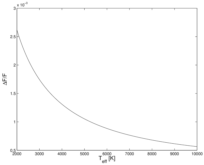
Figure 3: The amplitude of the expected beaming variability of a black-body radiation induced by the heliocentric motion of CoRoT, in the V band, assuming the star location is close to the ecliptic and the radial velocity amplitude is $60\,\mathrm{km\,s}^{-1}$.

The beaming photometric signal associated with the motion of the telescope will affect all stars, binary and single alike. Measuring this signal can serve to calibrate $\alpha$ with the radial-velocity amplitude, which in turn can be used to interpret the beaming signal of the stellar orbital velocity, if it is a binary. For single stars $\alpha$ is actually a piece of spectral information that reveals the location of the passband along the blackbody radiation curve, and thus provides an estimate of the stellar effective temperature. Figure 3 shows the expected photometric variability amplitude in V for different temperatures, due to heliocentric motion alone, assuming blackbody radiation law, and a heliocentric radial-velocity amplitude of $60\,\mathrm{km\,s}^{-1}$.

Figure 4 shows a simulated lightcurve that demonstrates the type of signal we expect to detect for a binary. The lightcurve includes the beaming variability of a $10$-day period G0-K0 binary star, together with the beaming variability related to the heliocentric motion. The associated radial velocity amplitudes are $K_{1}=52\,\mathrm{km\,s}^{-1}$ and $K_{2}=69\,\mathrm{km\,s}^{-1}$. The noise included is only a $10^{-4}$ white noise. Note that in the case of the heliocentric motion the contributions of the two components are in phase, and therefore do not cancel out.

Since the signal related to the observatory motion is common to all the observed objects, it will appear as a systematic effect, and may be mistakenly removed as such. Algorithms such as SysRem (Tamuz, Mazeh & Zucker, 2005) should identify such effects and also the individual response of each object to the same effect, and are thus ideally suited to provide the required information for its correct analysis.

In the lightcurve we show in Figure 4 we have neglected stellar microvariability. When actual lightcurves are analyzed, this variability should be properly accounted for. For older solar-type stars of low chromospheric activity, we may use the solar microvariability as the only available example. Although the solar rotational period is about $26$ days, Aigrain, Favata & Gilmore (2004) show that due to the short lifetimes of the spots and faculae, there is no clear periodic signal in this period. Instead, most of the signal is in higher frequencies, corresponding to periods shorter than $10$ days. For non-solar type stars, variability due to chromospheric activity may be larger than solar, and care should be taken in separating the beaming effects from the variability effects.

Efforts are currently underway to characterize the microvariability that we expect to observe with the high-precision photometric satellites (e.g., Aigrain, Favata & Gilmore, 2004; Lanza et al., 2006; Ludwig, 2006), in order to facilitate the detection of planetary transits. However, the stellar microvariability is not expected to be strictly periodic, and therefore it should be possible to single out the beaming effect, specially because the shape of the beaming modulation is known and depends only on a few parameters. Spectroscopic information obtained as part of the follow-up observations should also help to further study the chromospheric activity of the binary candidates.

In order to give an order-of-magnitude estimate of the expected number of beaming binaries that will be detected by, e.g., CoRoT, we estimate that $10\%$ of the observed late-types stars have been discovered to be spectroscopic binaries with a threshold of $K_{1}>3\,\mathrm{km\,s}^{-1}$ and periods of less than a year or so. This estimate is based on results of the seminal works of Duqennoy & Mayor (1991) and Latham et al. (2002). During the lifetime of the mission, CoRoT is expected to monitor about $60000$ stars. Thus, we roughly expect $6000$ of them to be detectable as beaming binaries with $10\mu$mag variability or higher. Since this estimate applies to binaries with late-type primaries, and accounting for the fact that beaming is biased against equal-mass binaries, we can somewhat scale this number downwards, and estimate CoRoT to yield at least $1000$ beaming binary stars. The fact that the CoRoT sample of beaming binaries will be discovered by a systematic, magnitude-limited survey, will augment significantly the statistical knowledge of binaries.

4 Conclusion

As we have shown in Section 2, we expect the multitude of very precise light curves of CoRoT and Kepler to yield hundreds of new binaries through their periodic beaming variability. Thus a new observational category will emerge — beaming binaries. In all types of binaries, the discovery and the analysis of the binary motion strongly depend on the timing and the number of the measurements. For the satellite photometric data we expect continuous radial-velocity data that will yield the spectroscopic orbital elements, the period and eccentricity in particular. Once the spectral index $\alpha$ is known, the radial-velocity amplitude can be derived as well.

Without the beaming binaries, CoRoT and Kepler are supposed to find most of the eclipsing binaries. However, binaries with periods longer than a few days need very fortuitous geometrical situations to present eclipses, and are therefore rare in the data of photometric surveys (e.g., Mazeh, Tamuz & North, 2006). The beaming binaries can be detected up to a hundred days and more. Therefore, the new class of binaries will extend our detailed knowledge of the statistical characteristics of binaries by an order of magnitude, specially because these binaries will emerge in the context of a well defined, complete, magnitude-limited, photometric search. This can shed light on the distribution of orbital period (e.g., Duqennoy & Mayor, 1991; Mazeh, Tamuz & North, 2006) and the relation between orbital period and eccentricity (e.g., Halbwachs et al., 2003).

Table 1: Stellar parameters for simulation

parameter	F0	G0	K0	Reference
Mass $[M_{\sun}]$	1.6	1.05	0.79	1
Radius $[R_{\sun}]$	1.5	1.1	0.85	1
Effective temperature $[\mathrm{K}]$	7300	5940	5150	1
Gravity darkening coefficient in V	0.9	0.4	0.4	2

References. — (1) Cox (2000) (2) Morris (1985)

Table 2: The three periodic photometric effects for sample binary configurations

		$P=10$ days			$P=100$ days
Primary	Secondary	ellipsoidal	reflection	beaming	ellipsoidal	reflection	beaming
F0	G0	$3.9\cdot 10^{-4}$	$4.8\cdot 10^{-4}$	$6.4\cdot 10^{-4}$	$3.9\cdot 10^{-6}$	$2.2\cdot 10^{-5}$	$2.9\cdot 10^{-4}$
F0	K0	$3.4\cdot 10^{-4}$	$4.1\cdot 10^{-4}$	$8.3\cdot 10^{-4}$	$3.4\cdot 10^{-6}$	$1.9\cdot 10^{-5}$	$3.8\cdot 10^{-4}$
G0	K0	$1.9\cdot 10^{-4}$	$2.1\cdot 10^{-4}$	$6.6\cdot 10^{-4}$	$1.9\cdot 10^{-6}$	$9.6\cdot 10^{-6}$	$3.1\cdot 10^{-4}$

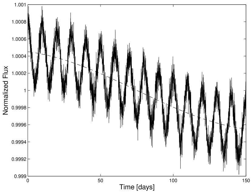
Figure 4: A simulated CoRoT lightcurve of a $10$-day period G0-K0 binary star. The beaming effects related to the binary orbit and the heliocentric motion are easily noticed. The dashed line represents the pure heliocentric motion beaming signal.

References

- Aigrain, Favata & Gilmore (2004) Aigrain, S., Favata, F., & Gilmore, G. 2004, A&A, 414, 1139
- Baglin (2003) Baglin, A. 2003, Adv. Space Res., 31, 345
- Barden & Armandroff (1995) Barden, S. C., & Armandroff, T. 1995, Proc. SPIE, 2476, 56
- Basri, Borucki & Koch (2005) Basri, G., Borucki, W. J., & Koch, D. 2005, New A Rev., 49, 478
- Cox (2000) Cox, A. N. 2000, Allen’s Astrophysical Quantities (New York: AIP)
- Duqennoy & Mayor (1991) Duquennoy, A., & Mayor, M. 1991, A&A, 248, 485
- Halbwachs et al. (2003) Halbwachs, J. L., Mayor, M., Udry, S., & Arenou, F. 2003, A&A, 397, 159
- Lanza et al. (2006) Lanza, A. F., Messina, S., Pagano, I., & Rodonò, M. 2006, AN, 327, 21
- Latham et al. (2002) Latham, D. W., Stefanik, R. P., Torres, G., Davis, R. J., Mazeh, T., Carney, B. W., Laird, J. B., & Morse, J. A. 2002, AJ, 124, 1144
- Loeb & Gaudi (2003) Loeb, A., & Gaudi, B. S., ApJ, 588, L117
- Ludwig (2006) Ludwig, H.-G. 2006, A&A, 445, 661
- Mazeh, Tamuz & North (2006) Mazeh, T., Tamuz, O., & North, P. 2006, MNRAS, 367, 1531
- Morris (1985) Morris, S. L. 1985, ApJ, 295, 143
- Morris & Naftilan (1993) Morris, S. L., & Naftilan, S. A. 1993, ApJ, 419, 344
- Pasquini et al. (2002) Pasquini, L., et al. 2002, Messenger, 110, 1
- Rybicki & Lightman (1979) Rybicki, G. B., & Lightman, A. P. 1979, Radiative Processes in Astrophysics (New York: Wiley)
- Tamuz, Mazeh & Zucker (2005) Tamuz, O., Mazeh, T., & Zucker, S. 2005, MNRAS, 356, 1466
- Zucker et al. (2006) Zucker, S., Alexander, T., Gillessen, S., Eisenhauer, F., & Genzel, R. 2006, ApJ, 639, L21
- Zucker & Mazeh (1994) Zucker, S., & Mazeh, T. 1994, ApJ, 420, 806