Unexpected relaxation dynamics of a self-avoiding polymer in cylindrical confinement

Abstract

We report extensive simulations of the relaxation dynamics of a self–avoiding polymer confined inside a cylindrical pore. In particular, we concentrate on examining how confinement influences the scaling behavior of the global relaxation time of the chain, $\tau$, with the chain length $N$ and pore diameter $D$. An earlier scaling analysis based on the de Gennes blob picture led to $\tau\sim N^{2}D^{1/3}$. Our numerical effort that combines molecular dynamics and Monte Carlo simulations, however, consistently produces different $\tau$–results for $N$ up to $2000$. We argue that the previous scaling prediction is only asymptotically valid in the limit $N\gg D^{5/3}\gg 1$, which is currently inaccessible to computer simulations and, more interestingly, is also difficult to reach in experiments. Our results are thus relevant for the interpretation of recent experiments with DNA in nano– and micro–channels.

I Introduction

Polymer chains immersed in solution are subject to constant molecular collisions and restlessly undergo conformational changes. Since the motion of each monomer or chain segment on a polymer is influenced by the rest, the polymer shows unique dynamical properties compared to those of simple molecules. Confinement in a pore or slit can change both the static and dynamic properties of a polymer chain qualitatively BdG . In the presence of cylindrical confinement, for instance, the pore diameter enters as an additional length scale. An early scaling approach BdG shows how this alters the relaxation dynamics.

One of the key concepts concerning polymer dynamics is the rate at which the modes relax DE ; deGennesBook ; Rubinstein ; Grosberg . Crudely speaking, this is a measure of the relative importance of each mode in describing the internal motion of a chain molecule. In particular, the longest relaxation time or the global relaxation time $\tau$ is of practical importance, as it determines how fast the chain reaches its equilibrium. Beyond this time, the internal motion plays no significant role, and the chain behaves just like a simple molecule.

A simple model for a polymer is the “ideal” chain, which is a phantom chain without self-avoidance. The Rouse model provides a description of its relaxation dynamics in an “immobile” solvent without hydrodynamic effects, and has been extended to the case of a free self–avoiding chain in the presence or absence of hydrodynamic effects DE ; deGennesBook ; Rubinstein ; Grosberg . In a similar spirit, the scaling behavior of a self–avoiding chain trapped in a pore of diameter $D$ has been studied BdG ; the trapped chain is viewed as a linear string of compression blobs deGennesBook ; BdG ; Rubinstein of diameter $D$.

The problem of a self-avoiding polymer under cylindrical confinement has relevance in a variety of contexts: DNA manipulations in nano– or micro–channels reisner , bacterial chromosome segregation future ; Jun06 , and polymer translocation through narrow pores Kasianowicz02 ; Dekker , to name a few. Additionally, the motion of such a polymer is reminiscent of reptation in concentrated polymer solutions deGennesBook ; DE . Consequently, this problem has been investigated in a number of simulation studies Takano ; Jendrejack ; chakraborty ; sheng ; KB before. However, to our knowledge, the asymptotic blob scaling prediction BdG for $\tau$ has never been directly confirmed.

In this work, we perform extensive simulations of a cylindrically confined chain, focusing on the slowest relaxation time $\tau$. The main goal is to examine dependence of $\tau$ on chain length $N$ and pore diameter $D$. For simplicity, we ignore hydrodynamic effects. Even with this simplification, the analysis of $\tau$ is quite nontrivial, as detailed below. In an effort to present a concrete picture, we combine molecular dynamics (MD) and Monte Carlo (MC) simulations. While the MD simulations permit a more direct probe into polymer dynamics, the MC simulations allow us to consider longer chains.

Despite the fact that we investigate a wide parameter space, we observe only an “intermediate” regime in our simulations, in which $\tau$ can be described by power laws with a much stronger $D$–dependence and a weaker $N$–dependence than the blob–scaling prediction. Interestingly, finite-size effects are more sensitively reflected in the dynamical quantity $\tau$; the static intermediate regime is much narrower than the dynamic counterpart. This intermediate regime might be relevant for the interpretation of single–molecule experiments on confined polymers, e. g., DNA in a nano– or micro–channel reisner .

This article is organized as follows. In Sec. II, we present a simple physical picture for describing the scaling behavior of the global relaxation time $\tau$ of a chain trapped in a cylindrical pore. The simulation methods employed in this work are described in Sec. III. Section IV is devoted to a detailed discussion on the results of the MD simulations and their analysis. In Sections VI and VII, we present results of our lattice (MC) simulations of the end-to-end distribution of the confined chain, from which we extract $\tau$ and compare it with the MD result presented in earlier sections. Finally, we discuss in Section VIII the implications of our results for single–molecule experiments on confined polymers.

II Theoretical background: Blob model and beyond

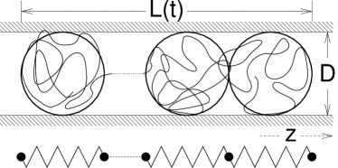
Figure 1: Cylindrically confined self–avoiding chain. In the blob picture, the chain is viewed as a linear string of compression blobs depicted as spheres. Inside each blob of diameter $D$, the effect of wall confinement is considered to be minor; beyond $D$, it tends to align the chain in the longitudinal direction, i. e., along the $z$ axis in our convention. For small deformations, the blobs are assumed to be deformed independently of each other, as illustrated by the series of springs in the lower figure.

Consider a linear self-avoiding chain consisting of $N$ monomers of size $a$, trapped in a cylindrical pore of diameter $D$ (see Fig. 1). In our convention, the $z$–axis coincides with the symmetry axis of the cylinder. If the longitudinal chain extension $L$ is much larger than $D$ and $D\gg a$, we can use the de Gennes blob model, which views the elongated chain as a string of self–avoiding compression blobs of diameter $D$ deGennesBook ; BdG ; deGennes .

Within a blob, the chain is expected to resemble a free or unconfined self-avoiding chain of $g$ beads. By equating $D$ with the “Flory radius” of the blob deGennesBook ; DE ; Flory that scales as $ag^{\nu}$, one obtains $g\sim(D/a)^{1/\nu}$, where footflory $\nu\approx 0.59$. Linear (i. e., longitudinal) ordering beyond $D$ demands that the total equilibrium or average chain extension $L_{\text{eq}}$ should scale as

$$L_{\text{eq}}=\left<L\right>\sim(N/g)D\sim Na^{\frac{1}{\nu}}D^{1-\frac{1}{\nu}},$$ (1)

where $\left<...\right>$ denotes an ensemble average. This scaling behavior has recently been confirmed in a theoretical approach thirumalai .

To estimate the longest relaxation time $\tau$ of the chain, we assume a Hookian–spring–like response to small excitations from the equilibrium length $L_{\text{eq}}$. If we know the effective spring constant $k_{\text{eff}}$ of the chain, the relaxation time is then reciprocally obtained as $\tau\sim N/k_{\text{eff}}$, where we have assumed that the chain friction is additive. For such small excitations, the spring constant of each blob should be BdG ; blob_spring_const $k_{b}\simeq k_{B}T/D^{2}$; here and in what follows, $k_{B}$ is the Boltzmann constant and $T$ is the temperature. We thus obtain

$$k_{\text{eff}}\sim\frac{k_{b}}{N_{\text{blobs}}}\sim\frac{k_{B}T}{a^{2}N\big{(}\frac{D}{a}\big{)}^{2-\frac{1}{\nu}}},$$ (2)

where $N_{\text{blobs}}=L_{\text{eq}}/D=N/g$ is the total number of blobs in the chain.

The mapping of the confined chain onto a series of Hookian springs used in Eq. 2 can be understood in analogy with a Rouse chain – beyond $D$, the confined chain resembles a one-dimensional Rouse chain BdG ; Takano . Slow Rouse modes are analogous to a random walk in a harmonic potential whose spring constant varies as $1/N$. The only difference is that in the confined case $N_{\text{blobs}}$ should be used in place of $N$, because now the blob–size $D$ is the smallest length scale for one-dimensional “Rouse deformations”.

Then, the global relaxation time is

$$\tau\sim\frac{\zeta N}{k_{\text{eff}}}\sim\frac{\zeta a^{\frac{1}{\nu}}}{k_{B}T}N^{2}D^{2-\frac{1}{\nu}},$$ (3)

where $\zeta$ is again the friction constant of each monomer. This derivation recovers the well-known result of Brochard and de Gennes BdG based on the blob picture. Hereafter, for simplicity, we use the following conventions: $\zeta=1,a=1,k_{B}T=1$. Then Eq. (1) becomes $L_{\text{eq}}=ND^{1-1/\nu}\approx ND^{-0.7}$, while Eq. (3) reduces to footexp $\tau\sim N^{2}D^{2-\frac{1}{\nu}}\approx N^{2}D^{0.3}$.

The effective spring constant $k_{\text{eff}}$ of a chain (or any elastic rod) can be obtained from its force-extension relation, from which the relaxation time $\tau$ can be deduced (Eq. 3). Alternatively, one can relate $k_{\text{eff}}$ to the equilibrium distribution of the end-to-end distance $L$, denoted by $p(L)$. The free energy cost for a small change in the chain length is a long–time potential effectively felt by the chain and determines the equilibrium distribution $p(L)$, which enables us to relate $k_{\text{eff}}$ to $p(L)$. For $L\approx L_{\text{eq}}=\left<L\right>$, the distribution $p(L)$ is Gaussian

$$p(L)=\frac{1}{\sqrt{2\pi}\sigma_{L}}\exp\left[-\frac{(L-L_{\text{eq}})^{2}}{2\sigma_{L}^{2}}\right],$$ (4)

where $\sigma_{L}$ is the variance of the distribution. This naturally arises from the assumption of a Hookian–spring–like response; the free energy should be $\sim(L-L_{\text{eq}})^{2}$ for $L\approx L_{\text{eq}}$. For large deformations, i. e., $L\ll L_{\text{eq}}$, however, the distribution does not have to remain symmetrical with respect to the line $L=L_{\text{eq}}$, as assumed in Eq. 4; see Sec. VI for details. The free energy cost for a global deformation is then $-k_{B}T\ln p(L)$, and one can thus establish $k_{\text{eff}}\simeq\left(\partial^{2}/\partial L^{2}\right)\left[k_{B}T\ln p(L)\right]=\sigma_{L}^{-2}$, which agrees with the equipartition theorem Landau . The relaxation time $\tau$ can then be related to the static quantity $\sigma_{L}$ as

$$\tau\sim\frac{N}{k_{\text{eff}}}\sim N\sigma_{L}^{2}.$$ (5)

Thus, the computation of $\tau$ boils down to that of $\sigma_{L}$.

III Simulation techniques

For the direct, dynamical measurements of the relaxation times, we employed an off-lattice Molecular dynamics (MD) simulation scheme together with a Langevin thermostat for a bead-spring model; to determine static properties such as the end-to-end distance distribution, we performed a lattice Monte-Carlo (MC) simulation that allows for efficient sampling of chain conformations. Below, we describe both simulation techniques.

III.1 MD details

In the MD simulations, we used a bead-spring model of polymers, which were trapped inside a long cylindrical tube with a circular or square cross section (we refer to the latter as “brick-shaped” confinement). The bead-bead and bead-wall interactions were modeled by the Weeks-Chandler-Andersen (WCA) potential wca (i.e., the repulsive part of the Lennard-Jones potential):

$$U_{\text{WCA}}(r)=\epsilon_{\text{WCA}}\left[\left(\frac{a}{r}\right)^{12}-\left(\frac{a}{r}\right)^{6}+\frac{1}{4}\right]$$ (6)

for $r<\sqrt[6]{2}a$ and 0 otherwise. Here $r$ denotes the center-to-center distance between two beads, or the distance of a bead center from the confining cylinder minus $a$ (i.e., the cylinder wall excludes the centers-of-mass of the beads). With our choice of $\epsilon_{\text{WCA}}=1\;k_{B}T$, this potential models soft beads of diameter $a$: their centers cannot come much closer to each other than $a$ and are confined to be on the inside of the confining wall. In the simulation, $a$ defines the basic length scale and $\epsilon_{\text{WCA}}$ the energy scale, i.e., we choose $a=1$ and $\epsilon_{\text{WCA}}=1k_{B}T$; in addition, we fix the mass scale so that the mass of each bead $m=1$. This automatically sets our basic time scale as $\tau_{\text{WCA}}=a\sqrt{m/\epsilon_{\text{WCA}}}=1$. Following the conventions in the theory section, we will henceforth omit the units of these quantities.

The bond between two neighboring beads, which endures chain connectivity, was modeled by the FENE (finite extensible nonlinear elastic) potential FENE

$$U_{F}(r)=-\frac{1}{2}4\epsilon_{F}\ln\left[1-\left(\frac{r}{2}\right)^{2}\right]\,,$$ (7)

where $r$ is again the distance of the bead centers and $\epsilon_{F}$ is the interaction strength. In the present simulations, we chose $\epsilon_{F}=10$, which in combination with the our WCA potential results in a typical bond length of $1.027$.

We simulated this system using the simulation package ESPResSo espresso . To integrate the equations of motion, we employed a velocity-Verlet MD integrator with a fixed time step of $0.01$; the system was kept at a constant temperature by means of a Langevin thermostat with a fixed friction of $\zeta=m\tau_{\text{WCA}}^{-1}=1$. The effect of the thermostat is not only to keep the temperature constant but also to ensure that each monomer moves diffusively, rather than ballistic. This is to mimic the effects of solvent viscosity in the high-damping limit, in which the inertia term can be dropped DE .

Initially, the chain was created as a biased, non-self-avoiding random walk confined within the pore. To equilibrate the system and remove possible bead-bead overlaps, we simulated the system for a few thousand steps with a truncated WCA potential. In other words, the WCA potential was modified such that the potential is linear for distances smaller than a certain cutoff radius. We reduced this cutoff gradually, until the potential had eventually converged to the full WCA interaction.

Next, we equilibrated the system further for a total equilibration time of $T_{\text{eq}}$, until the end-to-end distance and the radius of gyration had converged to their steady averages. This was followed by the sampling phase with a duration of $T_{\text{total}}$, during which we periodically recorded configurations for analysis. Between each two recorded configurations we waited for a time of $T_{\text{sample}}$ to reduce the statistical dependence of the configurations. For the parameters of the performed simulations, see Appendix A.

III.2 MC details

In an effort to sample a wide parameter space, we complement our MD simulations with lattice-based MC simulations. In our MC simulations, the polymers were modeled as a self-avoiding walk on a cubic lattice between hard walls forming the cylinder. In contrast to the MD simulations, where we typically used a cylindrical pore with a circular cross section, we mostly used one with a square cross section of area $D^{2}$ in the MC simulations. The latter is more compatible with the geometry of the cubic lattice (on which the polymer lives). Additionally, hard-core repulsions were defined as excluding conformations where two monomers occupy the same lattice site.

For the Monte Carlo moves, we adopted the “wormhole” method of Houdayer wormhole . This algorithm consists of a reptation-like motion so that the first bead jumps through a “wormhole” to a random position — not to be confused with reptation as a physical process in concentrated solutions DE ; deGennesBook . During the wormhole move, the polymer therefore consists of two disconnected segments. The reptation is continued, until a valid (i.e., connected) polymer conformation is obtained. This algorithm is known to be very efficient for sampling the chain conformations of polymers with excluded volume in confinement or in dense polymer melts. We only use this wormhole method to study static properties, since, by its nature, the dynamics based on this method is completely unphysical.

Between two chain conformations, we performed 1000 wormhole steps to assure statistical independence, and sampled in total 20,000 conformations per parameter set. Note that this algorithm requires no equilibration, because of the way it is constructed wormhole .

IV The end-to-end distance

Figure 2: Equilibrium chain extension $L_{\text{eq}}$ (in units of $R_{\text{F}}$) of a cylindrically confined self-avoiding chain as a function of the relative confinement $D/R_{\text{F}}$. The roman numbers denote the three regimes: the strong-confinement (I), intermediate (II), and free chain regime (III). The diagonal dashed line in regimes I and II represents the asymptotic power law $L_{\text{eq}}\sim ND^{-0.7}$, the dashed line in regime III corresponds to the free chain limit $L_{\text{eq}}=\sqrt{1/3}R_{\text{F}}$. The data points for $N$ up to 300 are MD results, while those for $N\geq 500$ are MC results.

If a chain is confined in an open cylinder with a diameter much smaller than its natural size, the chain will be stretched along the cylinder axis. Fig. 2 shows the confinement-induced chain stretching $L_{\text{eq}}/R_{\text{F}}$ as a function of the dimensionless parameter $D/R_{\text{F}}$. $L_{\text{eq}}$ denotes the equilibrium end-to-end distance parallel to the cylinder axis, and $R_{\text{F}}$ the Flory radius, i. e. the unconfined equilibrium end–to–end distance. In the figure, three different regimes are identified:

• To the region below $D\approx 0.2R_{\text{F}}$ we refer as the “strong” confinement regime, in which our simulation results are captured reasonably well by the scaling prediction $L_{\text{eq}}\sim ND^{1-1/\nu}\sim ND^{0.7}$. The data for large $N$ tend to follow this scaling better, because for small chains, the tube diameter approaches the size of the beads, in which case a “blob” only consists of a few beads.

• The range between $D\approx 0.2R_{\text{F}}$ and $D\approx R_{\text{F}}$, we denote as the “intermediate” confinement regime. In this regime, we find in our simulations a non-negligible chance for the chain to revert its direction along the cylinder axis or at least partially fold back one of its ends. Therefore, the average $L$ (or $L_{\text{eq}}$) decreases faster with increasing $D$ than what one may naively expect from the blob picture.

• In the region above $D\approx R_{\text{F}}$, the chain is essentially free; we call this therefore the “weak” confinement regime. Here, the chain extension is practically independent of $D$, and is given by $L=\sqrt{1/3}R_{\text{F}}$.

As we will argue below, the intermediate regime also appears in the behavior of the relaxation times $\tau$: however, it extends to much smaller values of $D/R_{\text{F}}$. Reaching the dynamic intermediate regime for $\tau$ therefore requires much larger chains than reaching its static counterpart for $L_{\text{eq}}$.

Note that, for the same number of monomers, the magnitude of $R_{\text{F}}$ is different for the lattice (MC) and off-lattice (MD) models. The $R_{\text{F}}$ obtained with the MD simulations is approximately $30\%$ larger than that found in the MC simulations. This difference can be absorbed into the effective monomer size $a$, which is proportional to $R_{\text{F}}$. Because $L_{\text{eq}}$ scales as $a^{1.7}$, this difference is more pronounced in the estimates of $L_{\text{eq}}$: for the same chain length and diameter, the chains in the MD simulations are about $60\%-100\%$ larger compared to the MC simulations.

V Relaxation time measurements

Figure 3: Global relaxation time $\tau_{\text{g}}$ of the radius of gyration $R_{\text{g}}$, in units of the relaxation time of a corresponding free chain, $\tau_{\text{g}}^{\text{free}}$) as a function of the reduced diameter $D/R_{\text{F}}$. The solid line marks the asymptotic scaling law of $\tau\sim N^{2}D^{0.3}$. The inset shows a graph $\tau_{\text{g}}/N^{2}$ vs $D$, demonstrating $\tau\sim N^{2}$ for small diameters.

We now turn to the global relaxation time $\tau$ of a confined polymer. In the case of strong confinement, one expects the blob–scaling result $\tau\sim N^{2}D^{2-1/\nu}\approx N^{2}D^{0.3}$ to be valid, in parallel with the static scaling law $L_{\text{eq}}\sim LD^{1-1/\nu}$. For weak confinement or $D\approx R_{\text{F}}$, one expects the scaling behavior of the relaxation time to cross over to that of a free polymer DE : $\tau\sim N^{1+2\nu}\approx N^{2.2}$. However, little is known about the relaxation time in the dynamic intermediate regime. Below we present the relaxation times determined in our simulations. As it turns out, we are not able to observe the expected blob–scaling for $\tau$, even for $D\ll 0.3R_{\text{F}}$. This indicates that the dynamic intermediate regime spans a much wider parameter space than the static intermediate regime.

We determine the relaxation time $\tau$ primarily from the slowest exponential decay of the autocorrelation function

$$C_{\text{g}}(t)=\frac{\left<(R_{\text{g}}(t)-\left<R_{\text{g}}\right>)(R_{\text{g}}(0)-\left<R_{\text{g}}\right>)\right>}{\left<R_{\text{g}}^{2}\right>-\left<R_{\text{g}}\right>^{2}},$$ (8)

where $R_{\text{g}}=(1/N)\sum_{i}\left(z_{i}-\left<z_{i}\right>\right)^{2}$ denotes the longitudinal component of the radius of gyration. The slowest exponential decay $\tau_{g}$ we obtained from fitting the long-time behavior of $C_{\text{g}}(t)\sim e^{-t/\tau_{\text{g}}}$. $\tau_{\text{g}}$ turns out to be rather insensitive to the exact definition of $R_{\text{g}}$; the relaxation time $\tau_{L}$ of the end-to-end distance differs from $\tau_{\text{g}}$ by less than $20\%$, and its overall behavior is the same ($\tau_{L}$-data not shown). We also determined the relaxation time by measuring the relaxation of a stretched chain. These relaxation times agree with the times obtained from the autocorrelation analysis, as expected on the basis of linear-response theory. However, the correlation function of the radius of gyration allows us to obtain better statistics. The global relaxation time $\tau_{\text{g}}$ obtained from our MD simulations is shown in Fig. 3.

For $D>0.5R_{\text{F}}$, $\tau_{\text{g}}$ quickly approaches that of a free chain. However, it has a maximum around $D\approx 0.5R_{\text{F}}$, beyond which the relaxation time decays slowly with increasing $D$ and eventually becomes $D$–independent for sufficiently large $D$. We argue that this non-monotonic behavior is associated with the reversion of the chain direction or chain back-folding. This process happens frequently in our simulations for $D>R_{\text{F}}$, and its timescale increases with decreasing $D$, as we will show below. Below $D=0.4R_{\text{F}}$, however, we do not observe any back-folding in our trajectories, so that the observed relaxation time is indeed dominated by the fluctuations of the chain length.

For $D\lessapprox R_{\text{F}}$, i.e., in the static intermediate and strong confinement regimes, the relaxation times we find in our MD simulations approximately scale as

$$\tau_{\text{MD}}\sim N^{1.75}D^{1.3}.$$ (9)

This result has a much stronger $D$–dependence and a slightly weaker $N$–dependence than the scaling result, which varies as $N^{2}D^{0.3}$. We refer to this as a dynamic intermediate regime, which spans deeply into the static strong confinement regime. We will present further analysis of this behavior based on blob statistics in Sec. VI.

In a small range in the static intermediate regime, we observe that the relaxation time increases more steeply with $D$ than indicated by the result in Eq. (9). However, this range quickly decreases with increasing chain length, and we will not consider it further. Note that in our simulations, we cannot consider diameters smaller than $D=2$. For narrower tubes, two beads can no longer pass each other without paying an energy penalty. This artifact significantly reduces the relaxation time, as can be seen from the anomalous behavior of $\tau_{\text{g}}$ towards the smallest $D/R_{\text{F}}$ values in Fig. 3 (see the data points at the left end of each curve). Also, in this case, $g\approx 1$, and thus the blob picture breaks down.

Figure 4: Global relaxation time $\tau_{z}$ obtained from the autocorrelation function of $L_{z}$, i.e., the longitudinal component of the end-to-end vector. The $\tau_{z}$ is given in units of the relaxation time $\tau_{z}^{\text{free}}$ of a corresponding free polymer. Our estimate of $\tau_{z}$ increases strongly with decreasing $D$, in contrast to $\tau_{\text{g}}$ plotted in Fig. 3.

To illustrate the significance of chain reorientation or back-folding in the weak confinement regime, we have plotted in Fig. 4 our results for the global relaxation time of the longitudinal end-to-end vector, the difference $L_{z}=z_{\text{head}}-z_{\text{tail}}$ of the $z$-coordinates of the head and tail beads (obviously, $L=|L_{z}|$). This relaxation time, denoted by $\tau_{z}$, is much longer than the $L$- or $R_{\text{g}}$-relaxation times; in our simulations, we were only able to track it down to $D/R_{\text{F}}\approx 0.4$. In the case of a free polymer, the relaxation times obtained from the fluctuations of its end-to-end vector and end-to-end distance are expected to be comparable to each other. In the presence of confinement, however, the distribution of $L_{z}$ has two minima at $L_{z}\approx\pm L_{\text{eq}}$, separated by a free energy barrier; these two minima correspond to the two possible chain orientations. In this case, chain reorientation, i. e. “tunneling” from one minimum to the other, represents the slowest mode. It requires a complete back-folding of the chain, which becomes unlikely with increasing chain length. Since the chain length increases with decreasing $D$, the reorientation timescale increases fast with $D$.

Figure 5: Comparison of two relaxation times: the global relaxation time $\tau_{\text{g}}$ of the longitudinal component of the radius of gyration, obtained from the autocorrelation function (filled symbols), and that from direct stretch-release simulations (open symbols). The dotted lines are guides to the eye.

As an alternative approach, we have determined the relaxation time from direct stretch–release simulations. In the linear-response regime, the relaxation times obtained from the autocorrelation function of the chain length should agree with the results of simulations that measure the relaxation of a slightly stretched chain. In order to show this, we carried out stretch-release simulations as follows. We started our simulations with equilibrated chains in confinement, whose end beads were initially fixed at a distance $L=L_{\text{eq}}+2\sigma_{L}$, where $\sigma_{L}^{2}$ is the variance of the chain length $L$. We then released the length constraint and recorded the time evolution of $L$, whose long-time behavior shows an exponential relaxation to its equilibrium value $L_{\text{eq}}$: $L(t)-L_{\text{eq}}\approx e^{-t/\tau_{L}}$ for large $t$. In Fig. 5, we have plotted the resulting $\tau_{L}$, together with the global relaxation time $\tau_{\text{g}}$ obtained from the autocorrelation function. While the two sets of data agree quite well with each other, the autocorrelation analysis yields better statistics. This analysis demonstrates the reliability of our results for $\tau_{\text{g}}$.

VI Linking between dynamics and statics: the $L$-distribution

Figure 6: MD results for the distribution of the end-to-end distance for $N=200$ and various pore sizes. The solid lines are Gaussian fits to the graphs.

The Molecular Dynamics simulations, that we have presented so far, are limited to chain lengths up to $N=300$, because the relaxation of longer chains in confinement becomes prohibitively slow. To circumvent this difficulty and to compliment the MD results, we carried out Monte Carlo (MC) simulations. Note that one cannot deduce dynamical information directly from the MC wormhole algorithm, since the artificial dynamics of this method relaxes the system nonphysically fast. However, for strong confinement, it is possible to connect the relaxation time, a dynamic quantity, to a static property, namely the distribution of the end-to-end distance, as illustrated in Sec. II.

In Fig. 6, we have plotted our MD results for the distribution of the end-to-end distance $L$, denoted by $p(L)$. As shown in the figure, this distribution is essentially Gaussian – the Gaussian fit works better for small $D$, i. e., in the strong confinement regime, as also indicated in Sec. II. For large $D$, $p(L)$ is only described well by the Gaussian in the region on the right side of the peak. The noticeable discrepancy towards the left end of the distribution can be attributed to partial chain back-folding, which tends to widen the distribution and creates an exponential tail.

Figure 7: Ratio of the relaxation time $\tau_{\text{g}}$ to $N\sigma_{L}^{2}$ obtained from MD simulations, as a function of the diameter $D/R_{\text{F}}$. As evidenced in the figure, this ratio tends to a $D$-independent constant ($\approx 0.1$) as $D$ decreases.

According to Eq. (5), the relaxation time is related to $\sigma^{2}_{L}$ via $\tau\sim N\sigma_{L}^{2}$ in strong confinement. This means that in this regime, the $D$ dependence of $\tau_{\text{g}}$ can be deduced from $\sigma_{L}$, since both have the same $D$-scaling. Fig. 7 shows the ratio of the relaxation time $\tau_{\text{g}}$ and the variance $N\sigma_{L}^{2}$ of the $L$-distribution, both obtained from the MD simulations. As expected, the ratio in the figure tends to a $D$-independent constant ($\approx 0.1$) as $D/R_{\text{F}}$ decreases. The non-monotonic $D$–dependence around $D\approx 0.3R_{\text{F}}$ is mainly due to a significant overshoot in $\sigma_{L}^{2}$ for $D\approx 0.5R_{\text{F}}$. This overshoot is caused by the widening of the $L$–distribution towards small $L$ due to the onset of chain reorientation or back-folding. Having established the relation $\tau\sim N\sigma_{L}^{2}$, we can focus on $\sigma_{L}^{2}$ and investigate its behavior more closely.

Figure 8: MD results for the end fluctuation $\sigma_{L}^{2}$ of a confined polymer, rescaled by $N$, as a function of $D$. The peaks are all located at $D\approx 0.5R_{\text{F}}$. The solid line represents the $D^{0.3}$-scaling expected from the blob approach. In the inset, $\sigma_{L}^{2}$ is rescaled by $N^{0.75}$, and the dashed line corresponds to $D^{1.3}$, in accordance with our best fit.

Figure 9: MC results for the end fluctuation $\sigma_{L}^{2}$ of a confined polymer, rescaled by $N$, as a function of $D$. The solid line represents the $D^{0.3}$-scaling expected from the blob approach. In the inset, $\sigma_{L}^{2}$ is rescaled by $N^{0.75}$, and the dashed line corresponds to $D^{0.75}$, in accordance with our best fit.

In Fig. 8 and 9, we represent our results for $\sigma_{L}^{2}$ from the MD simulations and the MC lattice simulations, respectively. The blob picture presented in Sec. II suggests that $\sigma_{L}^{2}$ scales as $ND^{0.3}$, i.e., $\sigma_{L}^{2}$ is extensive. However, both simulations indicate that $\sigma_{L}^{2}$ is not proportional to $N$, and has a much stronger $D$-dependence. More precisely, our data can be fitted well by $\sigma_{L}^{2}\approx N^{0.75}D^{1.3}$ for the MD simulations, and $\sigma_{L}^{2}\approx N^{0.75}D^{0.75}$ for the MC simulations. The main difference between the two sets of simulations is therefore the $D$–dependence; we will argue below that this is a lattice/off–lattice effect. While the MD result is consistent with $\tau$ in Eq. 9, the MC result leads to the estimate

$$\tau_{\text{MC}}\sim N^{1.75}D^{0.75}.$$ (10)

In the next section, we examine this unexpected scaling more carefully. For this, it proves useful to examine single-blob statistics, especially the variance $\sigma_{b}^{2}$ of the single-blob size distribution. This will enable us to investigate the $N$– and $D$–dependence of $\tau$ independently.

VII Analysis of single blobs

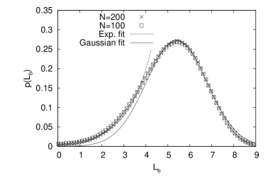
Figure 10: Typical blob size distribution for $D=5$ and chain lengths $N=100$ and $N=200$. A plain Gaussian distribution (solid line) fits the data well; for small $L_{b}$, the tail is better described by an exponential (dashed line).

To study our system at the level of a single blob, we determine the number of beads per blob $g$ from our simulations using the relation $L/D=N/g$ (Eq. (1)). We then view each sub-chain of beads $i+1,\ldots,i+g$, consisting of $g$ consecutive beads, as a realization of a blob. For example, we sample the distance $|z_{i+1}-z_{i+g}|$, i. e., the longitudinal distance between two “end” beads, as the “end-to-end” distance $L_{b}$ of a blob. In the strong confinement limit, the average size of a blob constructed this way is indeed $L_{b}\approx D$.

Fig. 10 shows our MD results for a typical blob size distribution $p(L_{b})$, which is well represented by a combination of two functions: a Gaussian distribution around the peak and an exponential one for small $L_{b}$. In this respect, the blob size distribution resembles a short chain in confinement $R_{\text{F}}\approx D$, as indicated in Fig. 6. In both cases, the effect of confinement is marginal and chain back-folding is noticeable, leading to the exponential distribution for small $L_{b}$. Furthermore, using both simulations (MD and MC), we found that the distribution of $L_{b}$ is practically independent of the chain length if $L>3D$, i.e., if the chain consists of at least 3 blobs.

Figure 11: MD and MC results for the ratio of the variances of the longitudinal end-to-end distance and the blob size, as a function of the number of blobs $N_{\text{blobs}}=N/g=L_{\text{eq}}/D$. The solid line represents the extensiveness $\sigma^{2}_{L}=\sigma^{2}_{b}N_{\text{blobs}}$ expected. Two types of confined space were used: a cylinder and a brick, i. e., a tube with a circular and rectangular cross section, respectively.

Figure 12: MD and MC results for the average variance $\sigma_{b}^{2}$ of the single blob size, as a function of the tube diameter $D$. As in Fig. 11, we used two types of confined space, a cylinder and a brick. The solid line represents the theoretically expected $D^{2}$-scaling.

Fig. 11 shows $\sigma_{L}^{2}/\sigma_{b}^{2}$, the ratio between the variances of the end-to-end distance and the blob size. If the fluctuations of the individual blobs are independent, this ratio should equal the number of blobs $N_{\text{blobs}}=N/g$, i. e., the end-to-end fluctuation is extensive. The data was obtained from both MD and MC simulations, and for two different shapes of the confined space each: a cylinder and a brick, i. e., a tube with a circular and square cross section, respectively. The discrepancy between the four cases is minor, however, we observe clear deviations from the linear relationship. The results in Fig. 11 for up to $N_{\text{blobs}}\approx 30$ are, in fact, better described by $\sigma^{2}_{L}/\sigma^{2}_{b}\sim N_{\text{blobs}}^{0.75}$. For large $N_{\text{blobs}}$, the data falls onto a line, however shifted up by about 1 and with a slope of about $0.9$. The shift is a finite-size effect that simply reflects that the size fluctuations of the two end–blobs are much larger. The slightly lower slope in turn indicates that the fluctuations between the blobs are not completely independent. We will discuss the implications of this finding below.

To further proceed with our discussion regarding the breakdown of extensiveness of the end fluctuation, we first focus on the variances $\sigma_{b}^{2}$, as shown in Fig. 12. We only took into account data points with $L>3D$, for which the chain length dependence of $L_{b}$ was negligible. The difference between the cylinder and the brick is again just an insignificant prefactor. However, while the shape of the $L_{b}$-distribution is very similar for the MD and MC simulations (i. e., approximately Gaussian), there are significant differences in the $D$–scaling of $\sigma^{2}_{b}$. The MC lattice simulations obey the theoretically expected $\sigma_{b}^{2}\sim D^{2}$ law (see Eqn. (2)) reasonably well, while in the MD simulations, $\sigma_{b}^{2}$ rather follows $\sigma_{b}^{2}\sim D^{2.6}$.

The most plausible explanation for this difference is through effects near the cylinder surface. The prediction $\sigma_{b}^{2}\sim D^{2}$ requires that the radial bead distribution can be written as a function of $\rho/D$ , where $\rho$ is the radial coordinate blob_spring_const . However, in the off–lattice simulations, we observe layering effects of the width of about a bead diameter at the cylinder surface, which are absent on the lattice layer . Because this surface layer for $D=6$ still contains about 30% of the total volume, this makes a significant contribution. Nevertheless, the radial distribution converges slowly to the universal distribution, and we expect the MD result to cross over to a $D^{2}$-law for sufficiently large $D$; unfortunately, this is computationally inaccessible.

The single-blob analysis presented in this section is consistent with the unexpected $D$–dependence of $\sigma^{2}_{L}$ (and that of the relaxation time): We observe $\sigma^{2}_{L}\approx(N/g)^{0.75}\sigma^{2}_{b}=N^{0.75}D^{-1.3}\sigma^{2}_{b}$, where $\sigma^{2}_{b}\sim D^{2.6}$ in the MD simulations and $\sigma^{2}_{b}\sim D^{2}$ in the MC simulations. In any case, $\sigma_{L}^{2}\propto\sigma_{b}^{2}$. This results in $\sigma^{2}_{L}\approx N^{0.75}D^{1.3}$ for the MD simulation and $\sigma^{2}_{L}\approx N^{0.75}D^{0.7}$ for the MC simulation, which are both in good agreement with our numerical findings for $\sigma^{2}_{L}$. Finally, when combined with our $\sigma_{L}$ analysis, the relation (5) leads to a relaxation time $\tau\sim N^{1.75}D^{1.3}$, again in good agreement with our earlier observations.

VIII Conclusions

We have performed extensive simulations of a self–avoiding polymer under cylindrical confinement. In an effort to sample a wide parameter space, we have complimented our off–lattice MD simulations by lattice MC simulations, and considered chain lengths $N$ up to $2000$. Most notably, both types of simulations have produced global relaxation times $\tau$ that have a much stronger $D$ dependence than expected from the earlier blob approach BdG . While our analysis of the longitudinal chain size $L$ for the case $D\lessapprox 0.2R_{\text{F}}$ tends to support the picture of linear ordering of blobs as assumed in the blob approach, our results for $\tau$ for the same case $D\lessapprox 0.3R_{\text{F}}$ do not show the dynamic blob scaling regime, in which the blob scaling of $\tau$ holds.

Our MD simulation directly measured the time evolution of the end–to–end distance from which $\tau$ was obtained; in our MC simulation we extracted $\tau$ from the variance of the end–to–end distance distribution $\sigma_{L}^{2}$ through the relation $\tau\sim N\sigma_{L}^{2}$, which we have demonstrated to hold in strong confinement. The absence of the dynamic blob–scaling regime in both types of simulations has been attributed to finite–size effects. To this end, we have examined the chain at the level of a single blob. In particular, we have examined the $D$–dependence of $\sigma_{b}^{2}$ and examined its relation with $\sigma_{L}^{2}$. Even with up to $N_{\text{blobs}}=30$ blobs, $\sigma_{L}^{2}=N_{\text{blobs}}\sigma_{b}^{2}$ does not hold. In other words, the assumption of extensiveness of $\sigma_{L}$, which underlies the blob picture, is not satisfied in our simulations. Moreover, the fluctuations of the individual blobs in our bead–spring model also suffer from finite size effects; in our MD simulations, we could not reach the expected $\sigma_{b}^{2}\sim D^{2}$ scaling due to large surface contributions. This indicates that the number of beads per blob also has to be significantly larger than 100, corresponding to a diameter which is at least 15 times larger than the effective bead diameter.

Our main findings can be summarized as

$$\tau\approx N^{1.75}D^{-1.3}\sigma_{b}^{2}.$$ (11)

When combined with our MD result $\sigma_{b}^{2}\approx D^{2.6}$ (obtained for $5\leq N\leq 300$ and $2\leq D\leq 15$), this relation leads to $\tau\approx N^{1.75}D^{1.3}$. If our MC result $\sigma_{b}^{2}\approx D^{2}$ (obtained for $200\leq N\leq 2000$ and $2\leq D\leq 20$) is used instead, we obtain $\tau\approx N^{1.75}D^{0.7}$. Both are quite different from the asymptotic scaling of $\tau\sim N^{2}D^{0.3}$. Nevertheless, our results for $\tau$ seem to hold for $0.05\leq D/R_{\text{F}}\leq 1$, and should therefore be experimentally observable.

Importantly, our simulations show that, for reaching the asymptotic scaling limit with a bead–spring model, about 10,000 beads are necessary. The aspect ratio $L/D$, which is identical to the number of blobs, has to be at least 30. The chain–length requirement for the asymptotic scaling regime $N\gg D^{1/\nu}\gg 1$ can then be satisfied, however, obtaining the relaxation of such a system by simulations will remain an intractable task for some time. For smaller chains and diameters, the blob-scaling picture has to be used with due caution. This is similar to recent findings for a polymer stretched by an external force without confinement Thirum , and for the force–stretching relation of a polymer in cylindrical confinement future2 .

In fact, we notice that even in experiments this regime is hard to reach. For instance, consider DNA molecules trapped in a cylindrical pore. Although the Kuhn segments of DNA are cylindrical and therefore our bead–model is not directly applicable, one can obtain some rough estimate on the minimally necessary system dimensions. To reach the classical self-avoiding polymer limit inside a blob of size $D$, this diameter has to be significantly larger than the persistence length of DNA, which is 50nm. Both our simulations and scaling analysis Rubinstein , indicate that a pore diameter of about 1$\mu$m is necessary. The extension of the chain in the pore should be at least 30 times the pore diameter, which requires a chain length of more than a million base pairs. This length is significantly larger than the 164,000 base pairs used in a recent experiment reisner .

Appendix A MD simulation parameters

In the following tables, we list the simulation parameters used for the different MD runs, namely the simulated pore diameters $D$, the equilibration times $T_{\text{eq}}$ and the sampling times $T_{\text{total}}$, as well as the time between two successive samples $T_{\text{sample}}$. The number of samples is hence given by $T_{\text{total}}/T_{\text{sample}}$. Times are measured in multiples of the microscopic time $\tau_{WCA}$, which corresponds to 100 MD time steps, i. e. the total number of performed time steps is equal to $100T_{\text{total}}$.

N=50
$D$ 2 2.5 3 3.5 4 6 8 10 $T_{\text{eq}}/10^{3}$ 1.2 4 4 4 3.2 5.2 8 10.8 $T_{\text{total}}/10^{6}$ 0.30 1.00 1.00 1.00 0.80 3.91 6.01 8.11 $T_{\text{sample}}$ 3 10 10 10 8 13 20 27
$D$ 14 20 60 $T_{\text{eq}}/10^{3}$ 9.95 9.95 20 $T_{\text{total}}/10^{6}$ 10.8 10.8 10.0 $T_{\text{sample}}$ 50 50 50

N=70
$D$ 2 2.5 3 3.5 4 6 8 10 $T_{\text{eq}}/10^{3}$ 2.4 3.2 4 5.2 6 10.4 16 20.8 $T_{\text{total}}/10^{6}$ 0.60 0.80 1.00 1.31 4.51 7.81 12.0 15.6 $T_{\text{sample}}$ 6 8 10 13 15 26 40 52
$D$ 14 20 60 $T_{\text{eq}}/10^{3}$ 20.8 100 40 $T_{\text{total}}/10^{6}$ 15.6 15.6 20.0 $T_{\text{sample}}$ 52 52 100

N=100
$D$ 2 2.5 3 3.5 4 5 6 8 $T_{\text{eq}}/10^{3}$ 4.8 6.8 8.8 10.8 12.4 16 22 28 $T_{\text{total}}/10^{6}$ 1.20 1.71 2.21 2.71 9.31 12.0 16.5 21.0 $T_{\text{sample}}$ 12 17 22 27 31 40 55 70
$D$ 10 12 14 16 20 30 40 $T_{\text{eq}}/10^{3}$ 34 100 300 500 500 800 1000 $T_{\text{total}}/10^{6}$ 25.5 30.0 30.0 30.0 30.0 29.4 30.0 $T_{\text{sample}}$ 85 100 100 100 100 100 100

N=150
$D$ 2 2.5 3 3.5 4 6 8 10 $T_{\text{eq}}/10^{3}$ 11.2 15.2 19.2 24 28 48 72 80 $T_{\text{total}}/10^{6}$ 2.81 3.82 4.82 6.02 7.03 12.0 7.98 7.57 $T_{\text{sample}}$ 28 38 48 60 70 120 180 200

N=200
$D$ 2 2.5 3 3.5 4 5 6 8 $T_{\text{eq}}/10^{3}$ 50 50 50 50 50 50 50 56 $T_{\text{total}}/10^{6}$ 2.89 4.09 5.30 5.42 6.22 8.03 9.94 13.4 $T_{\text{sample}}$ 24 34 44 54 62 80 110 140
$D$ 10 12 14 16 18 20 30 40 $T_{\text{eq}}/10^{3}$ 56 56 56 60 60 100 100 300 $T_{\text{total}}/10^{6}$ 14.5 14.1 14.1 15.1 15.1 12.1 12.1 12.1 $T_{\text{sample}}$ 170 140 140 150 150 200 200 200

N=300
$D$ 8 10 12 14 $T_{\text{eq}}/10^{3}$ 100 100 1000 2000 $T_{\text{total}}/10^{6}$ 30.1 30.1 30.1 30.1 $T_{\text{sample}}$ 200 200 200 200

N=200, box shaped simulation box
$D$ 2 3 4 5 6 7 8 9 $T_{\text{eq}}/10^{3}$ 9.6 17.6 24.8 32 40 44 48 52 $T_{\text{total}}/10^{6}$ 2.41 4.42 6.22 8.03 10.0 11.0 12.0 13.1 $T_{\text{sample}}$ 24 44 62 80 100 110 120 130

$D$	10	12	14	16
$T_{\text{eq}}/10^{3}$	52	56	56	60
$T_{\text{total}}/10^{6}$	13.1	14.1	14.1	15.1
$T_{\text{sample}}$	130	140	140	150

References

- (1) F. Brochard and P. de Gennes, J. Chem. Phys. 67, 52 (1977).
- (2) M. Doi and S. F. Edwards, The theory of polymer dynamics, Oxford Science Publications, 1986.
- (3) P. G. de Gennes, Scaling Concepts in Polymer Physics, Cornell University Press, 1979.
- (4) M. Rubinstein and R. Colby, Polymer Physics Oxford University Press, 2003.
- (5) A. Grosberg and A. R. Khokhlov, Statistical Physics of Macromolecules AIP Press, 1994.
- (6) K. Hagita and H. Takano, J. Phys. Soc. Japan 68, 401 (1999).
- (7) W. Reisner, K. Morton, R. Riehn, Y. M. Wang, Z. Yu, M. Rosen, J. C. Sturm, S. Y. Chou, E. Frey and R. H. Austin, Phys. Rev. Lett. 94, 196101 (2005).
- (8) S. Jun and B. Mulder, Proc. Nat. Acad. Sci. 103, 12388 (2006).
- (9) A. Arnold and S. Jun, Phys. Rev. E, accepted for publication.
- (10) A few relevant contributions can be found in J. J. Kasianowicz et al. (Editor), Structure and Dynamics of Confined Polymers, Kluwer Academic Publishers, 2002.
- (11) U. Keyser, C. Dekker et al., Nano Lett. 6, 89-95 (2006).
- (12) Y.-J. Sheng and M.-C. Wang, J. Chem. Phys. 114, 4724 (2000).
- (13) J. Kalb and B. Chakraborty, arXiv:cond-mat/0702152v1 (2007).
- (14) R. Jendrejack, D. Schwartz, M. Graham and J. de Pablo, J. Chem. Phys. 119, 1165 (2003).
- (15) K. Kremer and K. Binder, J. Chem. Phys. 81, 6381 (1984).
- (16) P. de Gennes, P. Pincus, and R. Velasco, J. Physique 37, 1461 (1976).
- (17) P. J. Flory, Principles of Polymer Chemistry, Cornell University Press, Ithaca, NY, 1953.
- (18) The original Flory exponent derived at the meanfield level Flory is , but we use the more accurate estimate DE .
- (19) G. Morrison and D. Thirumalai, J. Chem. Phys. 122, 194907 (2005).
- (20) The elastic free energy per blob, , can be Taylor–expanded for small deformations in powers of the longitudinal blob deformation . One obtains BdG , which leads to the blob spring constant given in the text.
- (21) If were used instead as in Ref BdG , one would reproduce the scaling result instead.
- (22) L. D. Landau and E. M. Lifshitz, Statistical Physics, 3rd Edt. Part 1, Butterworth-Heinemann, 1980.
- (23) J. D. Weeks, D. Chandler, and H. C. Andersen, J. Chem. Phys. 54, 5237 (1971).
- (24) T. Soddemann, B. Dünweg and K. Kremer, Eur. Phys. J. E 6, 409 (2001)
- (25) H.-J. Limbach, A. Arnold, B. A. Mann and C. Holm, Comp. Phys. Comm. 174, 704-727 (2006).
- (26) J. Houdayer, J. Chem. Phys. 116, 1783 (2002).
- (27) This layering is a consequence of the different shapes of the bead–bead radial distribution function. On the lattice, it is nonphysically flat, but off–lattice, it shows a significant peak at contact.
- (28) G. Morrison, C. Hyeon, N. M. Toan, B.-Y. Ha, and D. Thirumalai, to appear in Macromolecules (2007); see also arXiv:cond-mat/0705.3029v1 (2007).
- (29) S. Jun, A. Arnold and B.-Y. Ha, unpublished.