Where are the degrees of freedom responsible for black hole entropy?

Abstract

Considering the entanglement between quantum field degrees of freedom inside and outside the horizon as a plausible source of black hole entropy, we address the question: where are the degrees of freedom that give rise to this entropy located? When the field is in ground state, the black hole area law is obeyed and the degrees of freedom near the horizon contribute most to the entropy. However, for excited state, or a superposition of ground state and excited state, power-law corrections to the area law are obtained, and more significant contributions from the degrees of freedom far from the horizon are shown.

PACS Nos.: 04.60.-m,04.62.,04.70.-s,03.65.Ud

1 Introduction

The study of black holes (BHs) has always been a major testing arena for models of quantum gravity. The key issue has been to identify the microscopic origin of black hole entropy $S_{{}_{\rm BH}}$. The questions that naturally arise in this context are the following: (i) Why is $S_{{}_{\rm BH}}$, given by the well-known Bekenstein-Hawking relation [1, 2],

$$S_{{}_{\rm BH}}=\left(\frac{k_{{}_{B}}}{4}\right)\frac{\mathcal{A}}{\ell_{P}^{2}},\qquad\left(\ell_{{}_{P}}\equiv\sqrt{{\hbar G}/{c^{3}}}=\mbox{Planck length},~{}k_{{}_{B}}=\mbox{Boltzmann constant}\right)$$ (1)

is proportional to the horizon area $\mathcal{A}$, as opposed to volume (usual for thermodynamic systems)? (ii) Are there corrections to this so-called ‘area law’ (AL) and if so how generic are these corrections? (iii) Can we locate the degrees of freedom (DoF) that are relevant for giving rise to the entropy?

In the attempts to address these questions there have been two distinct approaches, viz., the one that associates $S_{{}_{\rm BH}}$ with fundamental DoF such as string, loop, etc. [3], and the other which attributes $S_{{}_{\rm BH}}$ to the entanglement of quantum field DoF inside and outside the BH event horizon [4, 5, 6, 7]. In this article we adopt the second approach and consider a quantum scalar field (in a pure state) propagating in the BH space-time. Since the BH horizon provides a boundary to an outside observer, the state restricted outside the horizon is mixed and leads to a non-zero entanglement (aka Von Neumann) entropy:  $S_{{}_{Ent}}=-k_{{}_{B}}$ Tr $\left(\rho\ln\rho\right)$, where $\rho$ is the mixed (or reduced) density matrix obtaining by tracing over the scalar DoF inside and outside the horizon.

In Ref. [4, 5] — for scalar field is in the vacuum/ground state (GS) — it was shown that $S_{{}_{Ent}}$ of scalar fields propagating in static BH and flat space-time (the DoF being traced inside a chosen closed surface) leads to the AL. In Refs. [8, 9, 10], the robustness of the AL is examined by considering non-vacuum states. It was shown that AL continues to hold for minimum uncertainty states like generic coherent state (GCS) or a class of squeezed states (SS), but for (1-particle) excited states (ES), or for a GS-ES superposition or mixing (MS), one obtains power-law corrections to the AL. Although for large horizon area, the correction term is negligible, for small BHs the correction is significant.

To understand physically the deviation from the AL for ES/MS, we ascertain the location of the microscopic DoF that lead to $S_{{}_{Ent}}$ in these cases [10, 11]. We find that although the DoF close to the horizon contribute most to the total entropy, the contributions from the DOF that are far from the horizon are more significant for ES/MS than for the GS. Thus, the corrections to the AL may, in a way, be attributed to the far-away DoF. We also extend the flat space-time analysis done in [5] to (curved) spherically symmetric static black-hole space-times.

In the next section, we first discuss the motivation for considering scalar fields for the entanglement entropy computations and then show that the scalar field Hamiltonian in a general BH space-time in Lemaître coordinates, and at a fixed Lemaître time, reduces to that in flat space-time. In sec. (3), we briefly review the procedure of obtaining the entanglement entropy and show the numerical results and estimations for the cases of GS, ES and MS. In sec. (4), we locate the scalar field degrees of freedom that are responsible for the entanglement entropy and compare the results for GS and ES/MS. We conclude with a summary and open questions in sec. (5).

In the following, we use units with $k_{{}_{B}}=c=\hbar=1$ and set $M_{{}_{\rm Pl}}^{2}=1/(16\pi G)$.

2 Hamiltonian of scalar fields in black-hole space-times

Scalar fields can be motivated from the viewpoint of gravitational perturbations in static asymptotically flat spherically symmetric space-time background with metric $g_{\mu\nu}$. For a metric perturbation $h_{\mu\nu}$, the linearized form of the Einstein-Hilbert action is invariant under the infinitesimal gauge transformation $h_{\mu\nu}\to h_{\mu\nu}+\xi_{(\mu;\nu)}$. Imposing the harmonic gauge condition, i.e., $\partial_{\mu}(2h^{\mu\nu}-g^{\mu\nu}h_{\alpha}^{\alpha})=0$ [12] and keeping only the first derivatives of $h_{\mu\nu}$, one finally obtains the linearized spin-2 equation [13]

$${\mathcal{S}}_{{}_{EH}}(g,h)=-\frac{M_{{}_{\rm Pl}}^{2}}{2}\int d^{4}x\sqrt{|g|}\,\nabla_{\alpha}{h}_{\mu\nu}\nabla^{\alpha}{h}^{\mu\nu}\,.$$ (2)

Assuming plane-wave propagation of the metric perturbations, i.e., $h_{\mu\nu}=M_{{}_{\rm Pl}}\epsilon_{\mu\nu}\varphi(x^{\mu})$ [$\epsilon_{\mu\nu}=$ polarization tensor], in the weak-field limit, the above action reduces to the action for a massless scalar field $\varphi$ propagating in the background metric $g_{\mu\nu}$:

$${\mathcal{S}}_{{}_{EH}}(g,h)=-\frac{1}{2}\int\!\!\!d^{4}x\sqrt{|g|}\,\partial_{\alpha}\varphi\partial^{\alpha}\varphi\,.$$ (3)

Hence, by computing the entanglement entropy of the scalar fields, we obtain the entropy of the metric perturbations of the background space-time. The Hamiltonian of a scalar field propagating in a general spherically symmetric space-time background with line-element:

$$ds^{2}=-A(\tau,\xi)\,d\tau^{2}+\frac{d\xi^{2}}{B(\tau,\xi)}+\rho^{2}(\tau,\xi)\left(d\theta^{2}+\sin^{2}\theta d\phi^{2}\right)\,,$$ (4)

$${\rm is~{}given~{}by}\qquad\quad H=\sum_{lm}\frac{1}{2}\int_{\tau}^{\infty}\!\!\!\!\!\!d\xi\!\left[\!\frac{\sqrt{AB}}{\rho^{2}}\Pi_{{}_{lm}}^{2}+\sqrt{AB}\,\rho^{2}(\partial_{\xi}\varphi_{{}_{lm}})^{2}+l(l+1)\sqrt{\frac{A}{B}}\,\varphi_{{}_{lm}}^{2}\right]\,,$$ (5)

where $A,B,\rho$ are continuous, differentiable functions of $(\tau,\xi)$ and we have decomposed $\varphi$ in terms of the real spherical harmonics $Z_{lm}(\theta,\phi)$, i.e., $\varphi(x^{\mu})=\sum_{lm}\varphi_{{}_{lm}}(\tau,\xi)Z_{lm}(\theta,\phi)$.

In the time-dependent Lemaître coordinates [13, 14] the line-element is given by (4) with $A(\tau,\xi)=1;~{}B^{-1}(\tau,\xi)=1-f(r);~{}\rho(\tau,\xi)=r(\tau,\xi)$. This line-element is related to that in the time-independent Schwarzschild coordinates by the following transformation relations [14]:

$$\tau=t\pm\int\!\!dr\frac{\sqrt{1-f(r)}}{f(r)}~{};~{}~{}\xi=t+\int\!\!dr\frac{[1-f(r)]^{-1/2}}{f(r)}~{}~{}~{}~{}~{}~{}\Rightarrow\xi-\tau=\int\frac{dr}{\sqrt{1-f(r)}}$$ (6)

As opposed to the Schwarzschild coordinate, the Lemaître coordinate is not singular at the horizon $r_{h}$, and $\xi$(or, $\tau$) is space(or, time)-like everywhere while $r$(or, $t$) is space(or, time)-like only for $r>r_{h}$. Choosing a fixed Lemaître time ($\tau=\tau_{0}=0$), the relations (6) lead to:  $d\xi/dr=1/\sqrt{1-f(r)}$. Plugging this in Eq.(5) and on performing the canonical transformations:  $\Pi_{{}_{lm}}\to{r\sqrt{1-f(r)}}\,\Pi_{{}_{lm}}\,;\,\varphi_{{}_{lm}}\to\varphi_{{}_{lm}}/r$, the Hamiltonian reduces to that of a free scalar field propagating in flat space-time [15]

$$H=\sum_{lm}\frac{1}{2}\int_{0}^{\infty}dr\left\{\pi_{lm}^{2}(r)+r^{2}\left[\frac{\partial}{\partial r}\left(\frac{\varphi_{lm}(r)}{r}\right)\right]^{2}+\frac{l(l+1)}{r^{2}}~{}\varphi_{lm}^{2}(r)\right\}.$$ (7)

This holds for any fixed $\tau$, provided the scalar field is traced over either the region $r\in(0,r_{h}]$ or the region $r\in[r_{h},\infty)$. Hence, evaluating the entanglement entropy of the scalar field in flat space-time corresponds to the evaluation of entropy of BH perturbations at a fixed Lemaître time.

3 Entanglement entropy of scalar fields

We discretize the scalar field Hamiltonian (7) on a radial lattice with spacing $a$:

$$H=\sum_{lm}H_{lm}=\sum_{lm}\frac{1}{2a}\sum_{j=1}^{N}\left[\pi_{lm,j}^{2}+\left(j+\frac{1}{2}\right)^{2}\left(\frac{\varphi_{lm,j}}{j}-\frac{\varphi_{lm,j+1}}{j+1}\right)^{2}+\frac{l(l+1)}{j^{2}}~{}\varphi_{lm,j}^{2}\right]\quad,$$ (8)

where $\pi_{lm,j}$ are the momenta conjugate of $\varphi_{lm,j}$, $(N+1)a$ is the infrared cut-off. $H_{lm}$ in Eq.(8) is of the form of the Hamiltonian of $N-$coupled harmonic oscillators (HOs):

$$H~{}=~{}\frac{1}{2}\sum_{i=1}^{N}p_{i}^{2}~{}+~{}\frac{1}{2}\sum_{i,j=1}^{N}x_{i}K_{ij}x_{j}\,,$$ (9)

where the interaction matrix $K_{ij}$ is given by:

$$K_{ij} = \frac{1}{i^{2}}\left[l(l+1)~{}\delta_{ij}+\frac{9}{4}~{}\delta_{i1}\delta_{j1}+\left(N-\frac{1}{2}\right)^{2}\delta_{iN}\delta_{jN}+2\left(i^{2}+\frac{1}{4}\right)\delta_{i,j(i\neq 1,N)}\right]$$ (10)

$$-\left[\frac{(j+\frac{1}{2})^{2}}{j(j+1)}\right]\delta_{i,j+1}-\left[\frac{(i+\frac{1}{2})^{2}}{i(i+1)}\right]\delta_{i,j-1}.$$

The last two terms denote nearest-neighbour interactions and originate from the derivative term in (7).

The most general eigenstate of the Hamiltonian (9) is a product of $N-$HO wave functions:

$$\psi(x_{1},\dots,x_{N})=\prod_{i=1}^{N}\frac{k_{Di}^{1/4}}{\pi^{1/4}~{}\sqrt{2^{\nu_{i}}\nu_{i}!}}~{}\mathcal{H}_{\nu_{i}}\left(k_{Di}^{1/4}~{}{\underline{x}}_{i}\right)\exp\left(-\frac{1}{2}k_{Di}^{1/2}~{}{\underline{x}}_{i}^{2}\right),$$ (11)

where ${\underline{x}}=Ux$, ($U^{T}U=I_{N}$), $K_{D}\equiv UKU^{T}$ (diagonal), and $\nu_{i}\,(i=1\dots N)$ are the indices of the Hermite polynomials ($\mathcal{H}_{\nu}$). The frequencies are ordered such that $k_{Di}>k_{Dj}$ for $i>j$.

The reduced density matrix is obtained by tracing over first $n$ of the $N$ oscillators:

$$\rho\left(x;x^{\prime}\right)=\int\prod_{i=1}^{n}dx_{i}~{}\psi(x_{1},\dots,x_{n};x_{n+1},\dots,x_{N})~{}\psi^{\star}(x_{1},\dots,x_{n};x^{\prime}_{n+1},\dots,x^{\prime}_{N})~{}.$$ (12)

It is not possible to obtain a closed form expression for $\rho(x;x^{\prime})$ for an arbitrary state (11). We resort to the following cases to compute the entropy numerically using the relation $S=$ Tr $\left(\rho\ln\rho\right)$:

(i) Ground state (GS) with $N$-particle wave-function:  $\psi_{0}(x;x^{\prime})\sim\exp\left[-\frac{1}{2}\sum_{i=1}^{N}k_{Di}^{1/2}{\underline{x}}_{i}^{2}\right]$.

(ii) Excited (1-particle) state (ES) with $N$-particle wave-function:  $\psi_{1}(x;x^{\prime})=\sqrt{2}\alpha^{T}K_{D}^{1/2}{\underline{x}}~{}\psi_{0}(x;x^{\prime})$, where $a^{T}=\left(a_{1},\dots,a_{N}\right)$ are the expansion coefficients and normalization of $\psi_{1}$ requires $a^{T}a=1$). We choose $a^{T}=1/\sqrt{o}(0,\cdots 0,1\cdots 1)$ with the last $o$ columns being non-zero.

(iii) GS-ES linearly superposed (i.e. mixed) state (MS) with $N$-particle wave-function:  $\psi(x;x^{\prime})=c_{0}\psi_{0}(x;x^{\prime})+c_{1}\psi_{1}(x;x^{\prime})$. Normalization of $\psi$ requires constants $c_{0}$ and $c_{1}$ related by $c_{0}^{2}+c_{1}^{2}=1$. For simplicity, we choose $c_{0}=1/2$. (See details in Ref. [10]).

Figure 1: (a) log(entropy) vs $\log(R/a)$ for GS, MS and ES (Eq/Hi). $R=a(n+1/2)$ is the horizon radius and $N=300,n=100-200,o=50$. (b) Plots of $S_{MS}/S_{GS},S_{ES}/S_{GS}$ and $S_{GS}/S_{MS},S_{GS}/S_{ES}$ (for $o=50$) with $\mathcal{A}$ to show the asymptotic nature of MS and ES entropies. (c) Best fit plots of $S_{MS}/S_{GS}$ vs $\mathcal{A}$ for $o=30,40,50$.

Results :  For GS, one recovers the AL — $S_{GS}\sim\mathcal{A}/a^{2}$, where $a$ is the ultraviolet cutoff at the horizon (set to be $\simeq\ell_{P}$). For MS and ES, we obtain power-law corrections to the AL:

$$S_{MS/ES}=S_{GS}+\sigma\left(\mathcal{A}/a^{2}\right)^{1-\nu}~{},$$ (13)

where $\sigma=$ constant of order unity and $\nu$ is a fractional index which depends on the excitation $o$. As the horizon area $\mathcal{A}$ increases, the correction term becomes negligible and $S_{MS}\rightarrow S_{GS}$ asymptotically. For small BHs, however, the correction is significant. Fig. 1 shows the logarithm of entropy versus log$(R/a)$ characteristics for GS, MS and ES ($R$ being the horizon radius), as well as the asymptotic equivalence of GS and MS/ES entropies, and the numerical fit that leads to the above result (13).

4 Location of the degrees of freedom

Let us take a closer look at the interaction matrix $K_{ij}$, Eq.(10), for the system of $N$ HOs. The last two terms which signify the nearest-neighbour (NN) interaction between the oscillators, are solely responsible for the entanglement entropy of black holes. Let us perform the following operations:

Figure 2: Plots of the percentage contribution $pc(q)$ to the total entropy as a function of window position $q$, for a window size $t=5$ and fixed $N=300,n=100$, in each of cases of GS, MS and ES. For MS and ES the solid curve is for $o=30$ whereas the broken curve is for $o=50$.

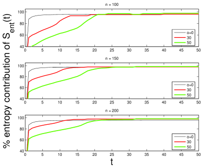
Figure 3: The left panels show the variations of the percentage contribution $pc(t)$ of total entropy with window width $t$ for GS ($o=0$) and ES (with $o=30,50$). The right panels show the plots of $\Delta pc(t)$ vs $n-t$ for GS and ES. Both sets of panels are for $N=300$ and $n=100,150,200$.

Operation I :  We set NN interactions to zero (by hand) everywhere except in a ‘window’, such that the indices $i,j$ run from $q-s$ to $q+s$, where $s\leq q$. We thus restrict the thickness of the interaction region to $t=2s+1$ radial lattice points, while allowing it to move rigidly across from the origin to a point outside the horizon. The variation of the percentage contribution of the total entropy $S_{tot}$ for a fixed window size of $t=5$ lattice points, i.e., $pc(q)=[S(q,t=5)/S_{tot}]\times 100$, as a function of $q$ is shown in Fig. 2 for $N=300,n=100$, in each of the cases GS and MS, ES with $o=30,50$. In all the cases $pc(q)=0$ when $q$ is far away from $n$ (i.e., horizon), whereas for values of $q$ very close to $n$ there are significant contributions to $S_{tot}$. For GS, $pc(q)$ peaks exactly at $q=n$. For MS and ES, however, the peaks shift towards a value $q>n$, and the amplitudes of the peaks also decrease as the amounts of excitation $o$ increase [11, 10]. Therefore (a) the near-horizon DoF contributes most to $S_{tot}$, and (b) the contributions from the far away DoF are more for MS and ES, than for GS.

Operation II :  We set the NN interactions to zero (by hand) everywhere except in a window whose center is fixed at $p\leq i,j\leq n$, and the window thickness $t\equiv n-p$ is varied from $0$ to $n$, i.e., from the origin to the horizon. For GS we find that about $85\%$ of the total entropy is obtained within a width of just one lattice spacing, and within a width of $t=3$ the entire GS entropy is recovered. Thus most of the GS entropy comes from the DoF very close to the horizon and a small part has its origin deeper inside. For ES, however, the total entropy is recovered for much higher values of $t$ (than for GS) since the DoF that are away from the horizon contribute more and more as the excitation $o$ increases. Thus larger deviation from the area law may be attributed to larger contribution to the total entropy from the DoF far from the horizon. The left panels of Fig. 3 depict the variation of the percentage contribution to the total entropy, i.e., $pc(t)=[S(t)/S_{tot}]\times 100$, as a function of $t$ for GS ($o=0$) and ES (with $o=30,50$). The situation is intermediate for MS (which interpolates between the GS and the ES), i.e., the total entropy is recovered for values of $t$ greater than that for GS, but less than that for ES (with same value of $o$). The percentage increase in entropy when the interaction region is incremented by one radial lattice point, $\Delta pc(t)=pc(t)-pc(t-1)$, versus $(n-t)$ plots for GS and ES are shown in the right panels of Fig. 3. In the case of GS the inclusion of the first lattice point just inside the horizon leads to an increase from $0$ to $85\%$ of the total GS entropy. The next immediate points add more to this, but the contributions are lesser and lesser with inclusion of points further and further from the horizon. For ES however, inclusion of one lattice point adds $70(50)\%$, for $o=30(50)$, to the entropy, while the next immediate points contribute more than those for the GS.

5 Conclusions

We have thus shown that if the black hole entropy is looked upon as that due to the entanglement between scalar field DoF inside and outside the horizon, there are power-law corrections to the Bekenstein-Hawking area law when the field is in excited state or in a superposition of ground state and excited state. Although such corrections are negligible for semi-classical BHs, they become increasingly significant with decrease in horizon area as well as for increasing excitations. The deviation from the AL for ES and MS may be attributed to the fact that the scalar field DoF that are farther from the horizon contribute more to the total entropy in the ES/MS cases than in the case of GS. The near horizon DoF contribute most in any case, however. We have also extended the flat space-time analysis done in [5] to static spherically symmetric black hole space-times with non-degenerate horizons.

We conclude with some open questions related to our work: (i) Can a temperature emerge in the entanglement entropy scenario and would it be consistent with the first law of BH thermodynamics? (ii) Is $dS/dt\geq 0$?, i.e., the second law of thermodynamics valid? (iii) Will the entanglement of scalar fields help us to understand the information loss problem? We hope to report on these in future.

Acknowledgments

SD and SSu are supported by the Natural Sciences and Engineering Research Council of Canada. SD thanks the organizers of Theory Canada III, Edmonton, AB, Canada for hospitality.

References

- [1] J. D. Bekenstein, Lett. Nuovo Cimento 4, 7371 (1972); Phys. Rev. D7, 2333 (1973); Phys. Rev. D9, 3292 (1974); Phys. Rev. D12, 3077 (1975).
- [2] S. W. Hawking, Nature 248, 30 (1974); Commun. Math. Phys. 43, 199 (1975).
- [3] A. Strominger, C. Vafa, Phys. Lett. B379, 99 (1996); A. Ashtekar et al, Phys. Rev. Lett. 80, 904 (1998); S. Carlip, ibid 88, 241301 (2002); A. Dasgupta, Class. Quant. Grav. 23, 635 (2006).
- [4] L. Bombelli, R. K. Koul, J. Lee, R. Sorkin, Phys. Rev. D34, 373 (1986).
- [5] M. Srednicki, Phys. Rev. Lett. 71, 666 (1993).
- [6] M. B. Plenio, Phys. Rev. Lett. 94, 060503 (2005); M. Cramer, J. Eisert, M.B. Plenio and J. Dreissig, Phys. Rev. A73, 012309 (2006).
- [7] R. Brustein, A. Yarom, Nucl. Phys. B709, 391 (2005); R. Brustein et al, JHEP 0601, 098 (2006).
- [8] M. Ahmadi, S. Das, S. Shankaranarayanan, Can. J. Phys. 84(S2), 1 (2006).
- [9] S. Das, S. Shankaranarayanan, Phys. Rev. D73, 121701 (2006); arxiv: gr-qc/0610022.
- [10] S. Das, S. Shankaranarayanan, S. Sur, arxiv: 0705.2070 (gr-qc).
- [11] S. Das, S. Shankaranarayanan, arxiv: gr-qc/0703082.
- [12] G. ’t Hooft and M. Veltman, Ann. Ins. Henri Poincaré A20, 69 (1975); N. H. Barth and S. M. Christensen, Phys. Rev. D28, 1876 (1983).
- [13] L. D. Landau, E. M. Lifshitz, Classical Theory of Fields, Pergamon Press, New York (1975).
- [14] S. Shankaranarayanan, Phys. Rev. D67, 084026 (2003).
- [15] K. Melnikov and M. Weinstein, Int. J. Mod. Phys. D13 1595 (2004).