A Galaxy Photometric Redshift Catalog for the Sloan Digital Sky Survey Data Release 6
Abstract
We present and describe a catalog of galaxy photometric redshifts (photo-z’s) for the Sloan Digital Sky Survey (SDSS) Data Release 6 (DR6). We use the Artificial Neural Network (ANN) technique to calculate photo-z’s and the Nearest Neighbor Error (NNE) method to estimate photo-z errors for 77 million objects classified as galaxies in DR6 with . The photo-z and photo-z error estimators are trained and validated on a sample of galaxies that have SDSS photometry and spectroscopic redshifts measured by SDSS, 2SLAQ, CFRS, CNOC2, TKRS, DEEP, and DEEP2. For the two best ANN methods we have tried, we find that 68% of the galaxies in the validation set have a photo-z error smaller than or . After presenting our results and quality tests, we provide a short guide for users accessing the public data.
Subject headings:
photometric redshifts sdss – Sloan Digital Sky Survey1. Introduction
While spectroscopic redshifts have now been measured for over one million galaxies, in recent years digital sky surveys have obtained multi-band imaging for of order a hundred million galaxies. Deep, wide-area surveys planned for the next decade will increase the number of galaxies with multi-band photometry to a few billion. Due to technological and financial constraints, obtaining spectroscopic redshifts for more than a small fraction of these galaxies will remain impractical for the foreseeable future. As a result, over the last decade substantial effort has gone into developing photometric redshift (photo-z) techniques, which use multi-band photometry to estimate approximate galaxy redshifts. For many applications in extragalactic astronomy and cosmology, the resulting photometric redshift precision is sufficient for the science goals at hand, provided one can accurately characterize the uncertainties in the photo-z estimates.
Two broad categories of photo-z estimators are in wide use: template-fitting and training set methods. In template-fitting, one assigns a redshift to a galaxy by finding the redshifted spectral energy distribution (SED), selected from a libary of templates, that best reproduces the observed fluxes in the broadband filters. By contrast, in the training set approach, one uses a training set of galaxies with spectroscopic redshifts and photometry to derive an empirical relation between photometric observables (e.g., magnitudes, colors, and morphological indicators) and redshift. Examples of empirical methods include Polynomial Fitting (Connolly et al. 1995), the Nearest Neighbor method (Csabai et al. 2003), the Nearest Neighbor Polynomial (NNP) technique (Cunha et al. 2007), Artificial Neural Networks (ANN) (Collister & Lahav 2004; Vanzella et al. 2004; d’Abrusco et al. 2007), and Support Vector Machines (Wadadekar 2005). When a large spectroscopic training set that is representative of the photometric data set to be analyzed is available, training set techniques typically outperform template-fitting methods, in the sense that the photo-z estimates have smaller scatter and bias with respect to the true redshifts (Cunha et al. 2007). On the other hand, template-fitting can be applied to a photometric sample for which relatively few spectroscopic analogs exist. For a comprehensive review and comparison of photo-z methods, see Cunha et al. (2007).
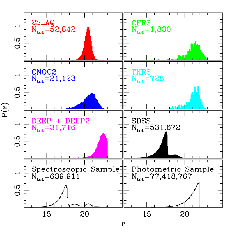
In this paper, we present a publicly available galaxy photometric redshift catalog for the Sixth Data Release (DR6) of the Sloan Digital Sky Survey (SDSS) imaging catalog (Blanton et al. 2003; Eisenstein et al. 2001; Gunn et al. 1998; Ivezić et al. 2004; Strauss et al. 2002; York et al. 2000). We use the ANN photo-z method, which we have shown to be a superior training set method (Cunha et al. 2007), and briefly compare the results using different photometric observables. We also compare the ANN results with those from NNP, an empirical method which achieves similar performance to the ANN method (Cunha et al. 2007). Since the SDSS photometric catalog covers a large area of sky, a number of deep spectroscopic galaxy samples with SDSS photometry are available to use as training sets, as shown in Fig. 1. In combination, these spectroscopic samples cover the full apparent magnitude range of the SDSS photometric sample.
The paper is organized as follows. In §2 we briefly describe the SDSS DR6 photometric catalog and the selection criteria used to obtain the galaxy photometric sample from the catalog. In §3 we describe the spectroscopic catalogs used to construct the photo-z training and validation sets. In §4 we outline the photo-z methods as well as the photo-z error estimator technique applied to the galaxy sample. Statistical results for photometric redshift performance, errors, and redshift distributions are presented in §5. In §6 we make recommendations for possible additional cuts on the photo-z catalog based on our own flags and those in the SDSS database. In §7 we briefly describe how to access the photo-z catalog from the public SDSS data server, and in §8 we present our conclusions. For completeness, Appendix A provides the database query used to select the photometric sample, Appendix B discusses issues of star-galaxy separation, and Appendix C briefly describes an earlier version of the photo-z algorithm used for SDSS DR5 (Adelman-McCarthy et al. 2007a).
2. SDSS Photometric Catalog and Galaxy Selection
The SDSS comprises a large-area imaging survey of the north Galactic cap, a multi-epoch imaging survey of an equatorial stripe in the south Galactic cap, and a spectroscopic survey of roughly galaxies and quasars (York et al. 2000). The survey uses a dedicated, wide-field, 2.5m telescope (Gunn et al. 2006) at Apache Point Observatory, New Mexico. Imaging is carried out in drift-scan mode using a 142 mega-pixel camera (Gunn et al. 2006) that gathers data in five broad bands, , spanning the range from 3,000 to 10,000 Å (Fukugita et al. 1996), with an effective exposure time of 54.1 seconds per band. The images are processed using specialized software (Lupton et al. 2001; Stoughton et al. 2002) and are astrometrically (Pier et al. 2003) and photometrically (Hogg et al. 2001; Tucker et al. 2006) calibrated using observations of a set of primary standard stars (Smith et al. 2002) observed on a neighboring 20-inch telescope.
The imaging in the sixth SDSS Data Release (DR6) covers an essentially contiguous region of the north Galactic cap, with only a few small patches remaining to be observed. In any region where imaging runs overlap, one run is declared primary111For the precise definition of primary objects see http://cas.sdss.org/dr6/en/help/docs/glossary.asp#P and is used for spectroscopic target selection; other runs are declared secondary. The area covered by the DR6 primary imaging survey, including the southern stripes, is , but DR6 includes both the primary and secondary observations of each area and source (Adelman-McCarthy et al. 2007b).
The SDSS database provides a variety of measured magnitudes for each detected object. Throughout this paper, we use dereddened model magnitudes to perform the photometric redshift computations. To determine the model magnitude, the SDSS photometric pipeline fits two models to the image of each galaxy in each passband: a de Vaucouleurs (early-type) and an exponential (late-type) light profile. The models are convolved with the estimated point spread function (PSF), with arbitrary axis ratio and position angle. The best-fit model in the band (which is used to fix the model scale radius) is then applied to the other passbands and convolved with the passband-dependent PSFs to yield the model magnitudes. Model magnitudes provide an unbiased color estimate in the absence of color gradients (Stoughton et al. 2002), and the dereddening procedure removes the effect of Galactic extinction (Schlegel et al. 1998).
| AB magnitude limits | RMS photometric | ||
|---|---|---|---|
| calibration errors | |||
| 22.0 | 2% | ||
| 22.2 | 3% | ||
| 22.2 | 2% | ||
| 21.3 | 2% | ||
| 20.5 | 3% | ||
Note. — Magnitude limits are for 95% completeness for point sources in typical seeing; 50% completeness numbers are generally 0.4 mag fainter (Adelman-McCarthy et al. 2007a). The median seeing for the SDSS imaging survey is .
To construct the photometric sample of galaxies for which we wish to estimate photo-z’s, we obtained a catalog drawn from the SDSS CasJobs website http://casjobs.sdss.org/casjobs/. We checked some of the SDSS photometric flags to ensure that we have obtained a reasonably clean galaxy sample. In particular, we selected all primary objects from DR6 that have the TYPE flag equal to (the type for galaxy) and that do not have any of the flags BRIGHT, SATURATED, or SATUR_CENTER set. For the definitions of these flags we refer the reader to the PHOTO flags entry at the SDSS website222http://cas.sdss.org/dr6/en/help/browser/browser.asp or to Appendix A. We also took into account the nominal SDSS flux limit (see Table 1) by only selecting galaxies with dereddened model magnitude . The full database query we used is given in Appendix A.
The photometric galaxy catalog we have selected suffers from impurity and incompleteness at some level, since the photometric pipeline cannot separate stars from galaxies with 100% success at faint magnitudes. We describe some of our tests of star/galaxy separation in Appendix B, where we show that the SDSS TYPE flag provides star/galaxy separation performance similar to other methods.
3. Spectroscopic Training and Validation sets
Since our methods to estimate photo-z’s and photo-z errors are training-set based, we would ideally like the spectroscopic training set to be fully representative of the photometric sample to be analyzed, i.e., to have similar statistical properties and magnitude/redshift distributions. Training-set methods can be thought of as inherently Bayesian, in the sense that the training-set distributions form effective priors for the analysis of the photometric sample; to the extent that the training-set distributions reflect those of the photometric sample, we may expect the photo-z estimates to be unbiased (or at least they will not be biased by the prior). Given the practical difficulties of carrying out spectroscopy at faint magnitudes and low surface brightness, such an ideal generally cannot be achieved. Realistically, all we can hope for is a training set that (a) is large enough that statistical fluctuations are small and (b) spans the same magnitude, color, and redshift ranges as the photometric sample. Fortunately, our tests indicate that the estimated photo-z’s depend only weakly on the shape of the redshift and magnitude distributions of the training set for the SDSS.

We have constructed a spectroscopic sample consisting of galaxies that have SDSS photometry measurements (counting repeats; see below) and that have spectroscopic redshifts measured by the SDSS or by other surveys, as described below. We imposed a magnitude limit of on the spectroscopic sample and applied additional cuts on the quality of the spectroscopic redshifts reported by the different surveys. Since we impose a limit of for the SDSS photometric sample, the fainter limit chosen for the spectroscopic training sample accommodates the full photometric range of interest without creating boundary effects for photo-z’s of galaxies with magnitudes near the photometric sample limit of . Each survey providing spectroscopic redshifts defines a redshift quality indicator; we refer the reader to the respective publications listed below for their precise definitions. For each survey, we chose a redshift quality cut roughly corresponding to 90% redshift confidence or greater. The SDSS spectroscopic sample provides redshifts, principally from the MAIN and Luminous Red Galaxy (LRG) samples, with confidence level . The remaining redshifts are: from the Canadian Network for Observational Cosmology Field Galaxy Survey (CNOC2; Yee et al. 2000), from the Canada-France Redshift Survey (CFRS; Lilly et al. 1995) with Class , from the Deep Extragalactic Evolutionary Probe (DEEP; Davis et al. 2001) with = A or B and from DEEP2 (Weiner et al. 2005)333http://deep.berkeley.edu/DR2/ with , from the Team Keck Redshift Survey (TKRS; Wirth et al. 2004) with , and LRGs from the 2dF-SDSS LRG and QSO Survey (2SLAQ; Cannon et al. 2006)444http://lrg.physics.uq.edu.au/New_dataset2/ with .
We positionally matched the galaxies with spectroscopic redshifts against photometric data in the SDSS BestRuns CAS database, which allowed us to match with photometric measurements in different SDSS imaging runs. The above numbers for galaxies with redshifts count independent photometric measurements of the same objects due to multiple SDSS imaging of the same region; in particular SDSS Stripe 82 has been imaged a number of times. The numbers of unique galaxies used from these surveys are from CNOC2, from CFRS, from DEEP and DEEP2, from TKRS, and from 2SLAQ. The SDSS spectroscopic samples were drawn from the SDSS primary galaxy sample and therefore are all unique. The spectroscopic sample obtained by combining all these catalogs, including the repeats, was divided into two catalogs of the same size ( objects each). One of these catalogs was taken to be the training set used by the photo-z and error estimators, and the other was used as a validation set to carry out tests of photo-z quality (see §4.1). Our tests indicate that this procedure of treating different images of the same training/validation set galaxies as independent objects leads to good results, provided all the photometric measurements for a given object are confined to either the training set or the validation set and not mixed. By contrast, excluding such multiple images from the spectroscopic sample would result in much smaller training and validation sets; these would be very sparse at faint magnitudes, leading to much diminished photo-z quality there. On the other hand, splitting the repeat images of a given object between the training and validation sets may result in “over-fitting” of the derived photo-z’s (see §4.1).
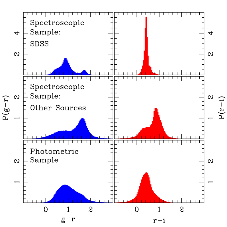
The -magnitude and color ( and ) distributions for the spectroscopic samples and for the photometric sample are shown in Figs. 1 and 2. While the magnitude and color distributions of the combined spectroscopic sample are not identical to those of the photometric sample, the spectroscopic sample does span the range of apparent magnitude and color of the photometric sample. To test the impact of having a training set that is not fully representative of the photometric sample, we divided the spectroscopic sample into smaller, alternate training and validation sets. For instance, to test the effect of the training-set magnitude distribution on the photo-z estimates, we created a training set with a flat magnitude distribution and another with an magnitude distribution similar to that of the photometric sample. Our tests indicated that the photo-z quality is not strongly affected by the magnitude distribution of the training set. The changes in the photo-z performance metrics (the rms scatter and the 68% CL region, defined below in §5) were smaller than when the training-set magnitude distribution was varied between these different choices. Since using the entire spectroscopic sample for the training and validation sets produced marginally better results than all other cases tested, we have adopted this as our final choice. In addition, we tested the effect of the size of the training set on our photo-z calculations. We found that the photo-z performance metrics defined in §5.1 are degraded by no more than 10% when the training set is artificially reduced to 10% of its original size. Even when the training set is reduced to of its original size, the photo-z performance metrics are degraded by less than . This gives us confidence that the spectroscopic training set size used here is sufficient for extracting nearly optimal photo-z estimates.
4. Methods
4.1. ANN and NNP Photometric redshifts
The ANN method that we use to estimate galaxy photo-z’s is a general classification and interpolation tool used successfully in an array of fields such as hand writing recognition, automatic aircraft piloting555http://www.nasa.gov/centers/dryden/news/NewsReleases/2003/03-49.html, detecting credit card fraud666http://www.visa.ca/en/about/visabenefits/innovation.cfm, and extracting astronomically interesting sources in a telescope image (Bertin & Arnouts 1996).
We use a particular type of ANN called a Feed Forward Multilayer Perceptron (FFMP) to map the relationship between photometric observables and redshifts. An FFMP network consists of several input nodes, one or more hidden layers, and several output nodes, all interconnected by weighted connections (see Fig. 3). We follow the notation of Collister & Lahav (2004) and denote a network with input nodes, nodes in hidden layer , and output nodes as . For each input object, the input photometric data (e.g., magnitudes, colors, concentrations, etc.) are fed into the input nodes of the FFMP, which fire signals according to the values of the input data. Each node in a hidden layer receives a total input which is a weighted sum of the outputs from the nodes in the previous layer, i.e., node in a hidden layer receives an input given by
| (1) |
where is the output of the node of the previous layer and is the weight of the connection between node in the hidden layer and node in the previous layer. Given the input , the output of node is a function of the input,
| (2) |
where is the activation function. Repeating this process, signals propagate up to the output nodes. The activation function is typically a sigmoid function:
| (3) |
However, there are various alternatives, such as step functions and hyperbolic tangents. Vanzella et al. (2004) show that the choice of activation functions makes no significant difference in the result.
We use :20:20:20:1 networks to estimate photo-z’s, where is the number of input photometric parameters per galaxy. The corresponding number of degrees of freedom (the number of weights) is roughly 1,000, depending on the actual value of . We use hyperbolic tangent functions as the activation function of the hidden layers and a linear activation function for the output layer.
Despite the occasional aura of mystery surrounding neural networks, an FFMP is nothing more than a complex mathematical function; in fact, one can always write down the analytic expression corresponding to a neural network function.
Once the network configuration is specified, it can be trained to output an estimate of redshift given the input photometric observables. The training process involves finding the set of weights that minimize a score function , chosen here to be
| (4) |
where is the measured spectroscopic redshift, is the output redshift of the output node, and the sum is over all galaxies in the training set. Note that the choice of score function is not unique, and different choices will in general lead to different photo-z estimates. The minimization of this score function can be done efficiently because its derivatives with respect to the weights are available analytically. We use a Variable Metric method as described in Press et al. (1992) for the minimization.
In machine learning, over-fitting refers to the tendency of an algorithm with many adjustable parameters to fit to the noise in the training set data. In order to avoid over-fitting, we use the technique of early stopping. The spectroscopic sample is divided into two independent subsets, the training and validation sets, and the formal minimizations are done using the training set. After each minimization step, the network is evaluated on the validation set, and the set of weights that performs best on the validation set is chosen as the final set. Another issue in machine learning is that minimization procedures that start at different initial choices of weights generally end at different local minima of the score function. To reduce the chance of ending in a less-than-optimal local minimum, we minimize five networks starting at different positions in the space of weights. Among these, we choose the network that gives the lowest photo-z scatter (cf. Eq. 4) in the validation set. For more details of our implementation of the ANN and its performance on mock catalogs and real data, see Cunha et al. (2007).
The ANN photo-z algorithm is very flexible in the sense that it is easy to change the input parameters, the training set, and the network configurations. We tried a variety of combinations of possible input photometric observables to see their effects on photo-z quality. We calculated photo-z’s using galaxy magnitudes, colors, and the concentration indices for some or all of the passbands. The concentration index in passband is defined as the ratio of PetroR50 and PetroR90, which are the radii that encircle 50% and 90% of the Petrosian flux, respectively. Early-type (E and S0) galaxies, with centrally peaked surface brightness profiles, tend to have low values of the concentration index, while late-type spirals, with quasi-exponential light profiles, typically have higher values of . Previous studies (Morgan 1958; Shimasaku et al. 2001; Yamauchi et al. 2005; Park & Choi 2005) have shown that the concentration parameter correlates well with galaxy morphological type, and we used it to help break the degeneracy between redshift and galaxy type. We present the photo-z results for different combinations of input parameters in §5.
For comparison, we also computed photo-z’s for the validation set using another empirical method, the Nearest Neighbor Polynomial (NNP) technique (Cunha et al. 2007). In NNP, to derive a photo-z for a galaxy in the photometric sample, we look for its training-set nearest neighbors in the space of photometric observables (magnitudes, colors, etc.). Suppose we have photometric data entries for each galaxy. The data vector for the galaxy of interest in the photometric sample is denoted by , while the data vector for the galaxy in the training set is . The distance between the photometric object and the training set galaxy is defined using a flat metric in data space,
| (5) |
The nearest neighbors are the training-set objects for which is minimum. Once the nearest neighbors for a given galaxy are identified, they are used to fit the coefficients of a local, low-order polynomial relation between photometric observables and redshift. The galaxy photo-z is then obtained by applying the derived relation to the photometric object.
For the NNP method employed in this work, we take the photometric data in Eq. (5) to be the four “adjacent” galaxy colors ; we found that this choice produces results marginally better than using the galaxy magnitudes. We use the nearest neighbors to fit a quadratic polynomial relation between redshift and the photometric data, here chosen to be the five magnitudes in each passband () and their corresponding concentration indices. We note that Wang et al. (2007) used a similar technique to estimate photo-z’s for a small sample of SDSS spectroscopic galaxies. They applied the Kernel Regression method of order 0, weighting the training-set neighbors and computing photo-z’s by using the weighted average of the neighbors’ redshifts. Our NNP method is closer to a Kernel Regression of order 2, since we perform quadratic fits; however, we do not apply variable weights to the neighbors but treat them equally in the fit.
Whereas the ANN method provides a single, nonlinear, global fit using the whole training set and applies the derived photo-z relation to all photometric objects, the NNP method yields a separate, linear (in parameters), local fit for each photometric object using its neighbors. If the galaxy magnitude-concentration-redshift hypersurface is a differentiable manifold, i.e., if it can be locally approximated by a hyperplane even though it is globally curved, then these two photo-z methods should be roughly equivalent. Indeed, as we show in §5, their performance is very similar.
4.2. Photometric redshift errors
We estimated photo-z errors for objects in the photometric catalog using the Nearest Neighbor Error (NNE) estimator (Oyaizu et al. 2007). The NNE method is training-set based, with a neighbor selection similar to the NNP photo-z estimator; it associates photo-z errors to photometric objects by considering the errors for objects with similar multi-band magnitudes in the validation set. We use the validation set, because the photo-z’s of the training set could be over-fit, which would result in NNE underestimating the photo-z errors.
The procedure to calculate the redshift error for a galaxy in the photometric sample is as follows. We find the validation-set nearest neighbors to the galaxy of interest. In contrast to NNP, where the distance in Eq. (5) was defined in color space, the NNE distance is defined in magnitude space, since photo-z errors correlate strongly with magnitude. Since the selected nearest neighbors are in the spectroscopic sample, we know their photo-z errors, , where is computed using the ANN or the NNP method. We calculated the width of the distribution for the neighbors and assigned that number as the photo-z error estimate for the photometric galaxy. Here we selected the nearest neighbors of each object to estimate its photo-z error. In studies of photo-z error estimators applied to mock and real galaxy catalogs, we found that NNE accurately predicts the photo-z error when the training set is representative of the photometric sample (Oyaizu et al. 2007).
4.3. Estimating the Redshift Distribution
As we shall see in §5.1, estimates for galaxy photo-z’s suffer from statistical biases that in general cannot be completely removed on an object-by-object basis. However, we can seek an unbiased estimate of the true redshift distribution for the photometric sample that is independent of individual galaxy photo-z estimates. For some statistical applications, the redshift distribution of the photometric sample, as opposed to individual galaxy photo-z’s, is all that is required. One way to estimate this distribution is to assign a weight to every galaxy in the spectroscopic sample such that the weighted spectroscopic sample has the same distributions of magnitudes and colors as the photometric sample. The distribution of this weighted spectroscopic sample provides an estimate of the true, underlying redshift distribution of the photometric sample.
The weight of the spectroscopic galaxy is calculated by comparing the local density around the galaxy in the spectroscopic sample with the density of the corresponding region in the photometric sample. The local density is evaluated by counting the number of nearest neighbors using the distance measured in the space of photometric observables, as in Eq. (5). We fix the number of spectroscopic neighbors, , which determines the distance to the -nearest spectroscopic neighbor. We then find the number of neighbors in the photometric sample within the same distance of the spectroscopic galaxy. Up to an arbitrary normalization factor, the weight is defined as
| (6) |
For our estimates, we chose , which provides a good match of the weighted spectroscopic distributions of magnitudes and colors to those of the photometric sample. We note that if additional cuts in magnitude or color are applied to the photometric sample, then this procedure must be repeated for the newly selected photometric sample. More details and tests of this method and comparisons with other methods for estimating the underlying redshift distribution (e.g., deconvolving the error distribution from the distribution) will be presented separately (Lima et al. 2007).


5. Results
5.1. Photometric redshifts
The photo-z precision (variance) and accuracy (bias) are limited by a number of factors. There are intrinsic degeneracies in magnitude-redshift space: low-luminosity, intrinsically red galaxies at low redshift can have apparent magnitudes similar to those of high-luminosity, intrinsically blue galaxies at high redshift. This natural degeneracy is amplified by photometric errors, since magnitude uncertainties propagate to photo-z errors. In addition to these observational limitations, which are determined by the photometric precision and the number of passbands of a survey, the photo-z estimator itself may have inherent limitations. For example, for training set methods, the size and representativeness of the training set are important factors, as are the number of parameters or weights in the fitting functions.
To test the quality of the photo-z estimates, we use four photo-z performance metrics. The first two metrics are the photo-z bias, , and the photo-z rms scatter, , both averaged over all objects in the validation set, defined by
| (7) | |||||
| (8) |
The third performance metric, denoted by , is the range containing of the validation set objects in the distribution of . This metric is useful because the probability distribution function is in general non-Gaussian and asymmetric (for a Gaussian distribution, and coincide). Explicitly, is defined by the value of such that 68% of the objects have . We also use the region , defined similarly. In addition to these global metrics, we also define local versions of them in bins of redshift or magnitude.
| Case | Inputs/Description | ||
|---|---|---|---|
| O1 | 0.0525 | 0.0229 | |
| C1 | + | 0.0519 | 0.0224 |
| D1 | + . Split training | 0.0519 | 0.0209 |
| CC1 | , , , | 0.0668 | 0.0272 |
| CC2 | , , , + | 0.0593 | 0.0245 |
Note. — Photo-z performance metrics and for the validation set using different input parameters (magnitudes, colors, and concentration indices) and training procedures.
To search for an optimal photo-z estimator, we computed photo-z’s using the ANN method with different combinations of input photometric observables. Five of these combinations are listed in Table 2. In the first case, dubbed O1, the training and photo-z estimation are carried out using only the five magnitudes . In case C1, we use the five magnitudes and the five concentration indices as the input parameters. In case CC1, we use only the four colors , , , and . In case CC2, we combine the four colors with the concentration indices in the filters. Finally, in case D1, we use the magnitudes and the concentration indices, but we split the training set and the photometric sample into 5 bins of magnitude and perform separate ANN fits in each bin. In all five cases, we use an ANN with three hidden layers and tune the number of hidden nodes to keep the total number of degrees of freedom of the network roughly the same for all cases.
Table 2 provides a summary of the performance results of the different ANN cases. We find that using concentration indices in addition to magnitudes (C1 vs. O1) helps break some degeneracies and reduces the photo-z scatter by a few percent. Using only colors (CC1) degrades the photo-z performance by as much as 20%, mostly because the degeneracy between intrinsically red, nearby galaxies and intrinsically blue, distant galaxies (with red observed colors) cannot be broken. Adding concentration indices to color-only training (CC2) helps break such a degeneracy, because the concentration index correlates with galaxy type and hence intrinsic color. Of the five, case CC2 also yields the most realistic photometric redshift distribution for the photometric sample (see §5.2). Finally, splitting the training set and photometric sample into magnitude bins (D1) produces results with the best performance metrics ( and ) of all the ANN cases we have tested. We choose D1 and CC2 as the best ANN cases and describe their results in more detail below; their outputs for the photometric sample are included in the public DR6 database.
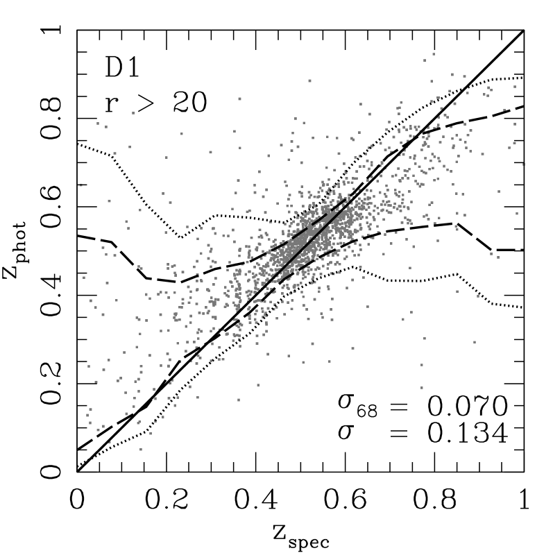
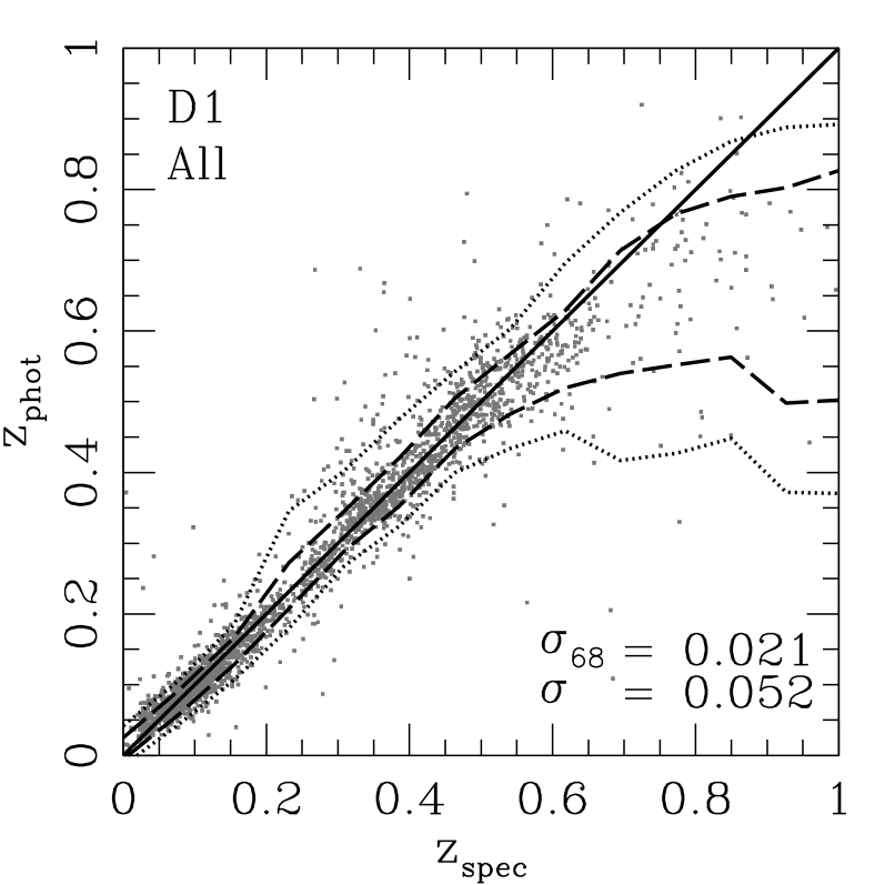
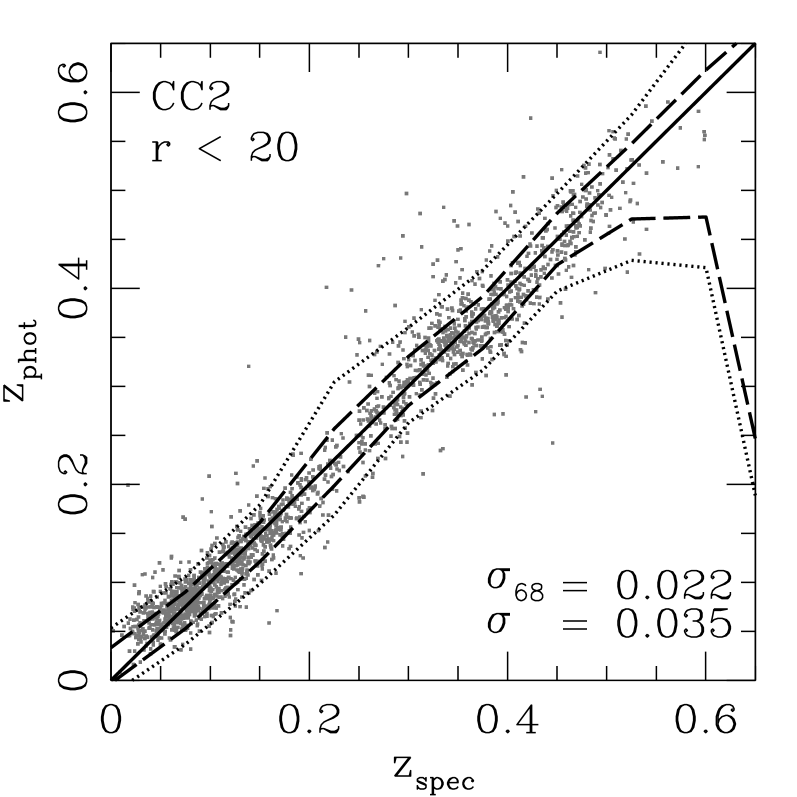
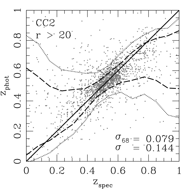
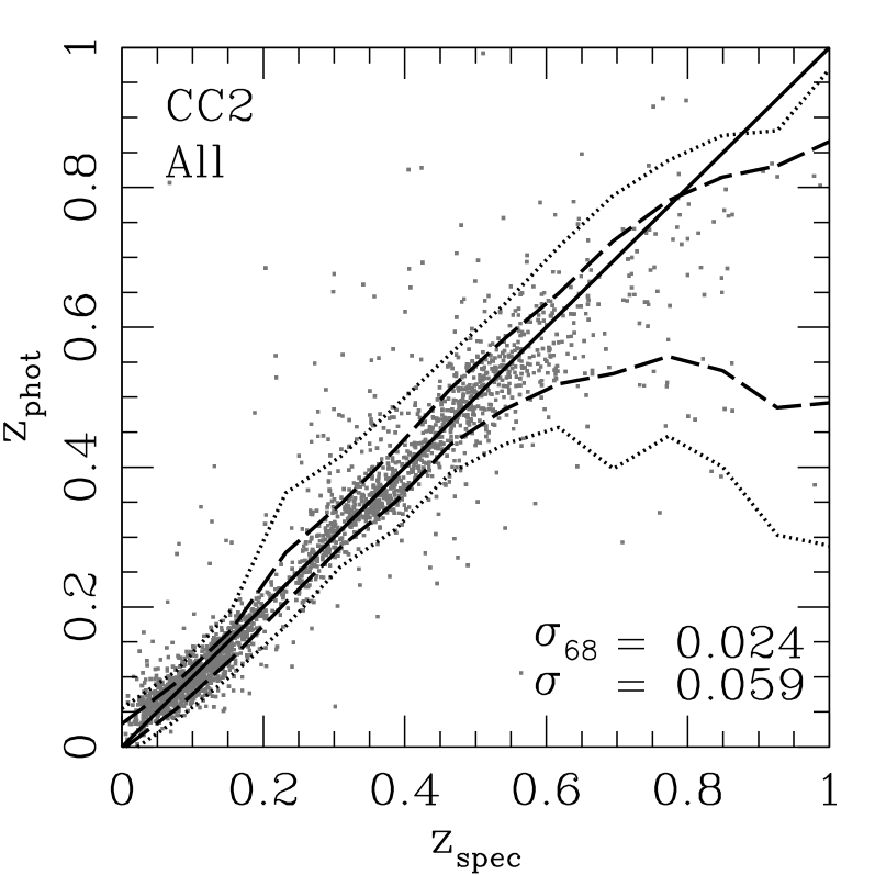
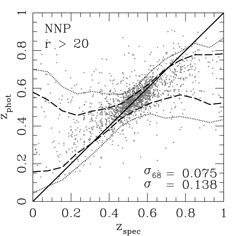
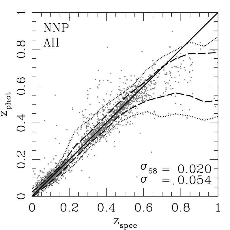
In Fig. 4, we plot photometric redshift, , for all objects in the validation set vs. true spectroscopic redshift, , for the different photo-z methods and cases and in different ranges of magnitude. The top row shows results for ANN case D1, the middle row shows the performance of ANN case CC2, and the bottom row shows results for the NNP method using magnitudes and concentration indices as the input parameters. In each panel, the values of the corresponding global photo-z performance metrics and are shown. The redshift bias is typically much smaller than or , since the photo-z methods are designed to minimize it (see Fig. 5). In each panel of Fig. 4, the solid line traces , i.e., the line for a perfect photo-z estimator. The dashed and dotted lines show the corresponding and regions, defined as above but in bins. Although each photo-z method probes the hypersurface defined by the photometric observables and redshift in a different way, they produce very similar results, suggesting that our results are limited not by the photo-z technique employed but by the intrinsic degeneracies in magnitude-concentration-redshift space and by the photometric errors.

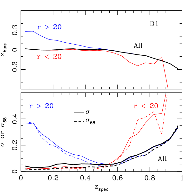
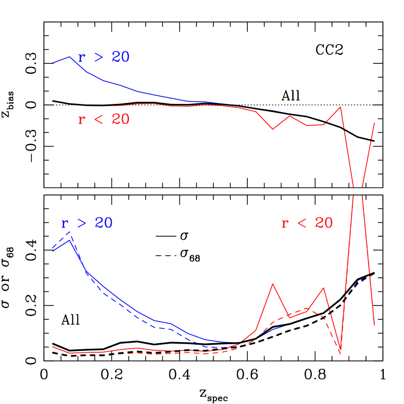

In Figs. 5 and 6, we show the performance metrics , , and as a function of magnitude and for the validation set for the two preferred ANN cases. We see that the photo-z precision degrades considerably for objects with . This increased scatter is expected, since the relative photometric errors increase as the nominal detection limit of the SDSS photometry is approached (see Table 1). While the bias for CC2 increases at , we note that the fraction of objects in the photometric sample which are that bright is very small. As a function of redshift, and increase dramatically beyond for the validation set. For the part of the sample, the number of spectroscopic objects with is simply too small to characterize the redshift-magnitude surface, as shown in the left panel of Fig. 7. For the faint objects (), the scatter is low for between 0.4 and 0.6 and increases outside of that range. It’s important to note that the photo-z performance metrics were calculated independently of spectral type. Since the the neural network and the training set were not optimized for any specific galaxy population (e.g., galaxies in clusters) it is possible that certain galaxy types may have photo-z’s with worse (or better!) biases and dispersion.
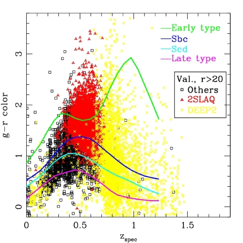
In Figure 7, we plot color versus spectroscopic redshift for the validation set for both bright () and faint () galaxies. The 2SLAQ and DEEP2 galaxies are highlighted by different colors (shades of grey), and the expected color-redshift relations for the four spectral templates from Coleman et al. (1980) (from early to late types) are indicated by the solid lines. We see that for the faint sample, in the range , the galaxies come mostly from the 2SLAQ survey, which used specific color cuts to select early-type galaxies at . Because early-type galaxies have a well-defined 4000 Å break feature, their photo-z’s are well determined and their photo-z scatter is low. Outside of the range , the validation set at faint magnitudes is dominated by bluer galaxies that do not have strong, broad spectral features, resulting in the larger photo-z scatter seen in Fig. 6.
Fig. 6 shows that the common assumption that the photo-z scatter scales as is not consistent with our estimates for the SDSS sample. The functional form of the scatter versus redshift depends strongly on the underlying galaxy type distribution.
5.2. Redshift Distributions
So far, we have considered the scatter and bias of photo-z estimates. As discussed in §4.3, it is also of interest to consider the predicted photo-z distribution as a whole. Different photo-z estimators may achieve similar values for the metrics , , and , but predict different forms for the photo-z distribution of the photometric sample. As we shall see, this is the case with the two ANN cases D1 and CC2. We therefore define two additional performance metrics to quantify the quality of the predicted photo-z distribution. The first metric, , measures the rms difference between the binned and distributions of the validation set,
| (9) |
where is the height of the redshift bin of the distribution, is the height of the same redshift bin of the distribution, and is the total number of redshift bins used. Here we use equally spaced redshift bins running from to .
The second redshift distribution metric we employ is the KS statistic , the maximum value of the absolute difference between the two ( and ) cumulative redshift distribution functions. An advantage of the KS statistic is that it does not require binning the data in redshift. However, our use of the KS statistic to quantify the difference between the and distributions of the validation set likely does not adhere to formal statistical practice, since it turn outs that the probability for the KS statistic for both cases we consider is very close to zero (Press et al. 1992).
Table 3 shows the values of and of the KS statistic for the validation set for the D1 and CC2 ANN photo-z’s, for different ranges of magnitude. Although the CC2 photo-z distribution is a worse overall match to the distribution for the validation set, it works better than D1 for . Since the photometric sample is dominated by objects at (see Fig. 1), these results suggest that CC2 should do a better job in estimating the redshift distribution of the photometric sample, even though D1 performs better by the standards of and .
| KS statistic | |||||
| -mag bin | CC2 | D1 | CC2 | D1 | |
| 0.0392 | 0.0330 | 0.0632 | 0.0391 | ||
| 0.0390 | 0.0430 | 0.0520 | 0.0533 | ||
| 0.0391 | 0.0399 | 0.0366 | 0.0413 | ||
| 0.0403 | 0.0471 | 0.0363 | 0.0665 | ||
| 0.0652 | 0.0702 | 0.1051 | 0.1306 | ||
| All | 0.0383 | 0.0338 | 0.0485 | 0.0307 | |
Note. — and KS statistic results for CC2 and D1 ANN photo-z’s for the validation set.
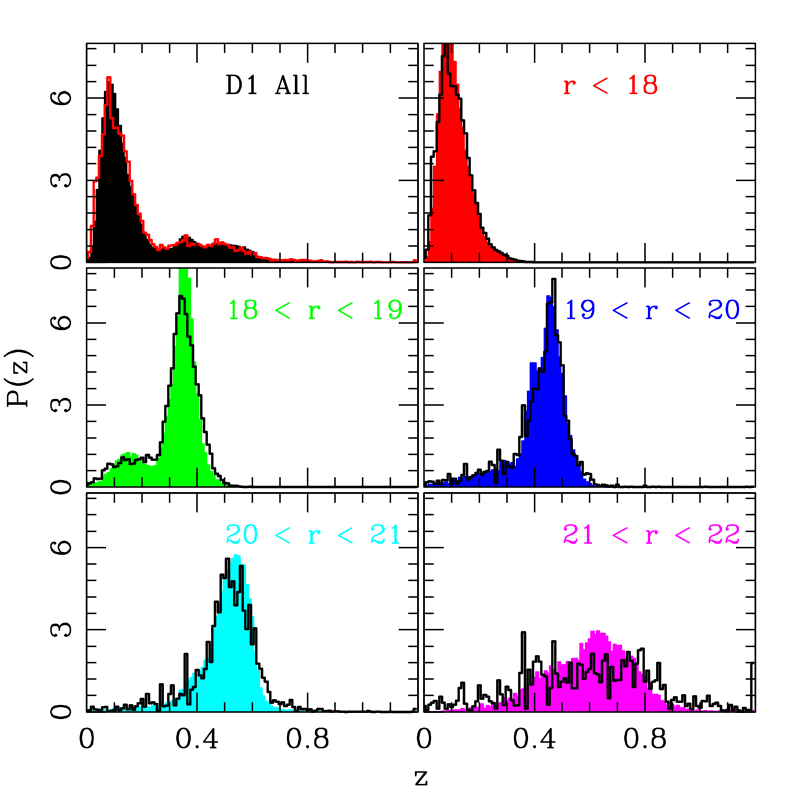
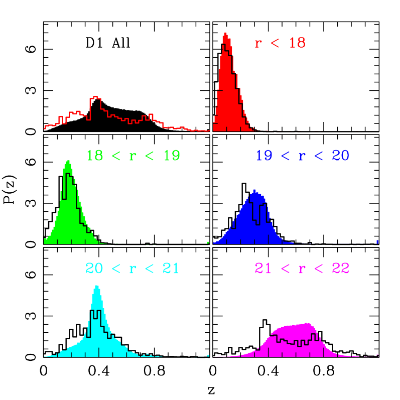
The redshift distributions for the validation set are shown in Fig. 8 for the same bins of magnitude as in Table 3. The D1 and CC2 distributions are shown in color, and the solid curves correspond to the distributions. The similarities between the and distributions are consistent with the results of Table 3.
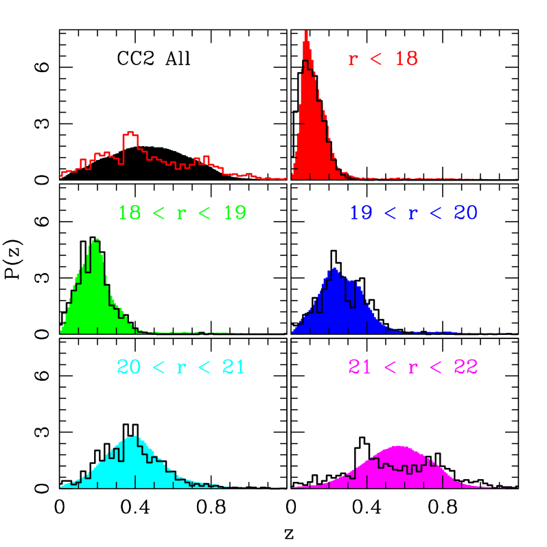
In §4.3, we noted that the distribution of the spectroscopic sample, weighted to reproduce the color and magnitude distributions of the photometric sample, provides an estimate of the unknown redshift distribution of the photometric sample. The distribution for the photometric sample, computed using ANN D1 or CC2, provides another estimate of the true redshift distribution for the photometric sample, but one that we know suffers from bias (e.g., Fig. 5). While we have not shown that the weighted estimate of the redshift distribution is unbiased, it has the advantage that it makes direct use of the statistical properties of the photometric sample, and we believe it is our best estimate of the photometric sample redshift distribution. Our final test of photo-z performance therefore compares the distribution for the photometric sample for the two ANN cases with the weighted distribution of the spectroscopic sample. Agreement between the weighted distribution and either one of the distributions does not guarantee that they are correct, but it at least provides a useful consistency check.
In Fig. 9 we show the estimated redshift distributions of a random subsample containing of the objects in the DR6 photometric sample for both the CC2 and D1 ANN cases. The colored regions correspond to the distributions, and the solid lines indicate the weighted distribution of the spectroscopic sample. The distributions for CC2 are closer matches to the weighted distributions for , and they do not show the peculiar features that the D1 photo-z distributions display, particularly at faint magnitudes. By the criterion of producing a more realistic redshift distribution for the photometric sample, the CC2 ANN estimator is preferred.
5.3. Photo-z Errors
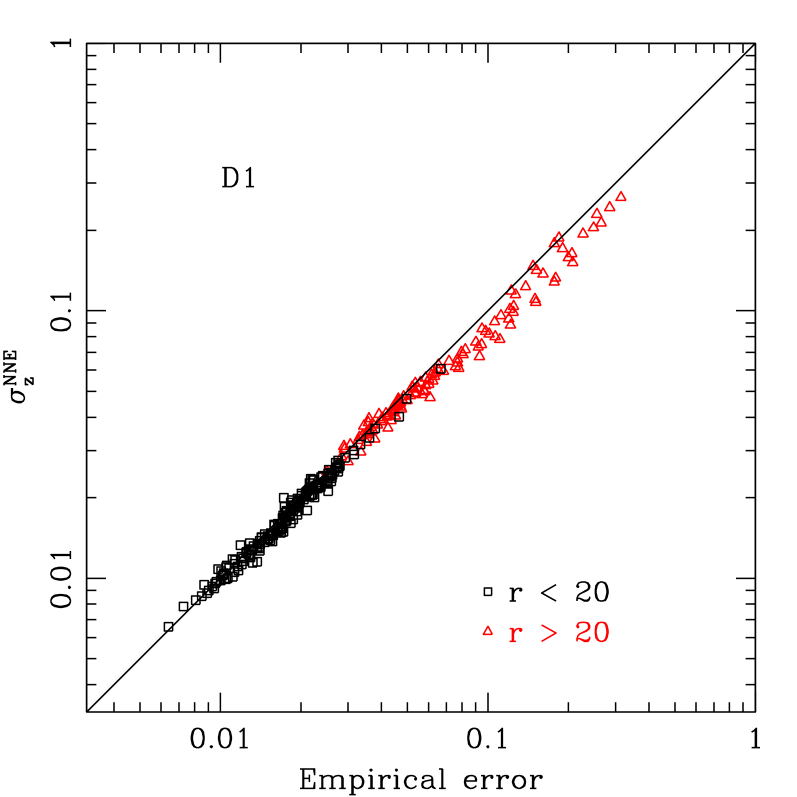
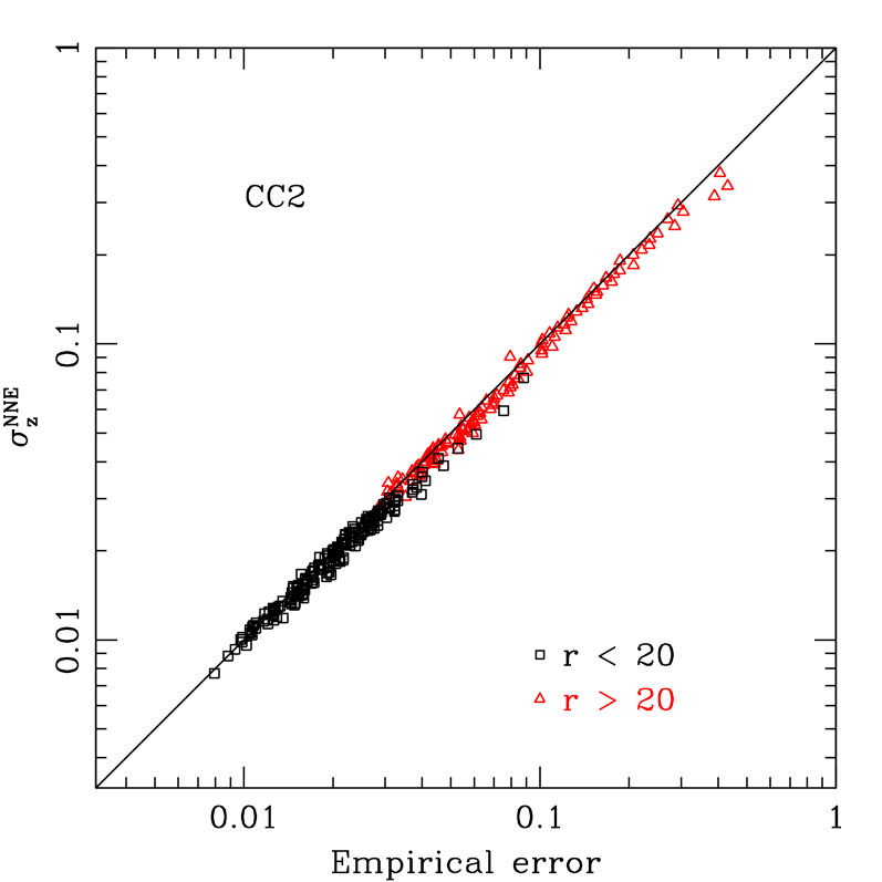
In order to test the quality of our photo-z error estimates calculated with the NNE method, we introduce the concept of empirical error. For a set of objects (within the validation set) with similar NNE error, , the empirical error is defined as the width of the distribution for the set. If the NNE estimator works properly, objects with similar NNE error should have similar underlying error distributions, i.e., the NNE error should correlate well with the empirical error.
Fig. 10 shows the performance of the photo-z error estimator by plotting the computed NNE error as a function of the corresponding empirical error for the validation set. Results are shown for the D1 and CC2 ANN photo-z’s. The empirical error was calculated for bins containing objects with similar . As expected, faint objects () have larger errors than bright objects (). The NNE estimated error correlates well with the empirical error even for the faint objects, indicating that the error estimator works properly for all magnitudes. The bulk of the bright objects have in the range , consistent with the overall rms photo-z scatter of indicated in Fig 4. Likewise, faint objects have in the range , while for those objects. The NNE error is therefore a robust indicator of an object’s photo-z quality. In particular, we have carried out tests in which we cut objects with large NNE error from the sample and found that the remaining sample has smaller photo-z scatter and fewer catastrophic outliers. For applications in which photo-z precision is more important than completeness of the photometric sample, this can be a useful procedure.

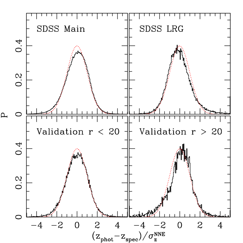
In Fig. 11, we plot the normalized error distribution, i.e., the distribution of , for objects in the spectroscopic sample, using the D1 ANN estimator. The solid black lines are the data, and the dotted red lines show Gaussian distributions with zero mean and unit variance. The upper panels show results for the galaxies in the SDSS Main and LRG spectroscopic samples. The lower panels show results for all validation-set galaxies, divided into bright () and faint () samples. These plots indicate that, averaged over the bulk of the spectroscopic sample, the photo-z estimates are nearly unbiased, the NNE error provides a good estimate of the true error, and the NNE error can be approximately interpreted as a Gaussian error in this average sense. Note that this does not imply that the photo-z error distributions in bins of magnitude or redshift are unbiased Gaussians: Figs. 5 and 6 show that they are not.
6. Query Flags and Caveats
When querying the SDSS data server to produce the photometric sample for which we estimated photo-z’s, we set the most relevant flags needed to produce a clean galaxy sample. However, some applications may require more stringent selection of objects. We advise users of the catalog to read the documentation about producing a clean galaxy sample on the SDSS website777 http://cas.sdss.org/dr6/en/help/docs/algorithm.asp . In particular, users should consider requiring the BINNED1 (object detected at ) flag and removing objects with the NODEBLEND (object is a blend but deblending was not possible) flag. The various PHOTO flags are described in more details at the above website as well as in Appendix A.
Finally, we note that the training of the photo-z estimators included only galaxies, not stars. As a result, photo-z estimates for stars that contaminate the photometric sample will be wrong, and cutting objects with low will not remove them. Our tests on star/galaxy separation in the photometric sample are briefly described in Appendix B.
7. Accessing the Catalog
The photo-z catalog can be accessed from the photoz2 table in the DR6 context on the SDSS CasJobs site, at http://casjobs.sdss.org/casjobs/. A query similar to the one in the Appendix provides all objects for which we computed photo-z’s. Alternatively, one can simply perform a query that searches for objects with a photoz2 entry.
8. Conclusions
We have presented a public catalog of photometric redshifts for the SDSS DR6 photometric sample using two different photo-z estimates, CC2 and D1, based on the ANN method. As a consistency check, we have also calculated photo-z’s using the NNP method, a nearest neighbor approach, which gives very good agreement with the ANN results. The CC2 and D1 photo-z results are comparable. For the validation set, the D1 photo-z estimates have lower photo-z scatter for bright galaxies (), and scatter similar to but slightly smaller than that of CC2 for objects with . Our tests indicate that the SDSS photo-z estimates are most reliable for galaxies with and that the scatter increases significantly at fainter magnitudes. For faint galaxies (), we recommend using the CC2 photo-z estimate, since the CC2 distribution most closely resembles the distribution for the validation set and the weighted estimate for the redshift distribution of the photometric sample. For users who wish to use, for simplicity, a single photo-z estimator over the full magnitude range, we recommend using CC2.
Finally, we have demonstrated that the NNE error estimator, included in the public catalog, provides a reliable measure of the photo-z errors and that the overall scaled photo-z errors are nearly Gaussian.
Funding for the DEEP2 survey has been provided by NSF grant AST-0071048 and AST-0071198. The data presented herein were obtained at the W.M. Keck Observatory, which is operated as a scientific partnership among the California Institute of Technology, the University of California and the National Aeronautics and Space Administration. The Observatory was made possible by the generous financial support of the W.M. Keck Foundation. The DEEP2 team and Keck Observatory acknowledge the very significant cultural role and reverence that the summit of Mauna Kea has always had within the indigenous Hawaiian community and appreciate the opportunity to conduct observations from this mountain.
Funding for the SDSS and SDSS-II has been provided by the Alfred P. Sloan Foundation, the Participating Institutions, the National Science Foundation, the U.S. Department of Energy, the National Aeronautics and Space Administration, the Japanese Monbukagakusho, the Max Planck Society, and the Higher Education Funding Council for England. The SDSS Web Site is http://www.sdss.org/.
The SDSS is managed by the Astrophysical Research Consortium for the Participating Institutions. The Participating Institutions are the American Museum of Natural History, Astrophysical Institute Potsdam, University of Basel, University of Cambridge, Case Western Reserve University, University of Chicago, Drexel University, Fermilab, the Institute for Advanced Study, the Japan Participation Group, Johns Hopkins University, the Joint Institute for Nuclear Astrophysics, the Kavli Institute for Particle Astrophysics and Cosmology, the Korean Scientist Group, the Chinese Academy of Sciences (LAMOST), Los Alamos National Laboratory, the Max-Planck-Institute for Astronomy (MPIA), the Max-Planck-Institute for Astrophysics (MPA), New Mexico State University, Ohio State University, University of Pittsburgh, University of Portsmouth, Princeton University, the United States Naval Observatory, and the University of Washington.
Appendix A Data Query Code
Here we provide the SDSS database query used to obtain part of the catalog containing the photometric sample used in this paper. Notice that the query requires the TYPE flag to be set to 3 (galaxies) and selects objects with dereddened model magnitude to reflect the SDSS nominal detection limit. The query to obtain objects with Right Ascension (RA) in the range is
declare @BRIGHT bigint set @BRIGHT=dbo.fPhotoFlags(’BRIGHT’)
declare @SATURATED bigint set @SATURATED=dbo.fPhotoFlags(’SATURATED’)
declare @SATUR_CENTER bigint set @SATUR_CENTER=dbo.fPhotoFlags(’SATUR_CENTER’)
declare @bad_flags bigint set @bad_flags=(@SATURATED|@SATUR_CENTER|@BRIGHT)
select
objID, ra, dec,type,dered_u,dered_g,dered_r,dered_i,dered_z,
petroR50_u, petroR50_g, petroR50_r, petroR50_i, petroR50_z,
petroR90_u, petroR90_g, petroR90_r, petroR90_i, petroR90_z
into MyDb.all_ra_0_170
FROM PhotoPrimary
WHERE ((flags & @bad_flags)) = 0 AND (dered_r<=22.0) AND (ra>=0.0) AND (ra<170.0)
AND (type = 3)
Here we provide a brief description of the flags used in the query: BRIGHT indicates that an object is a duplicate detection of an object with signal to noise greater than ; SATURATED indicates that an object contains one or more saturated pixels; SATUR_CENTER indicates that the object center is close to at least one saturated pixel. Note that in selecting PRIMARY objects (using PhotoPrimary), we have implicitly selected objects that either do not have the BLENDED flag set or else have NODEBLEND set or nchild equal zero. In addition, the PRIMARY catalog contains no BRIGHT objects, so the cut on BRIGHT objects in the query above is in fact redundant. BLENDED objects have multiple peaks detected within them, which PHOTO attempts to deblend into several CHILD objects. NODEBLEND objects are BLENDED but no deblending was attempted on them, because they are either too close to an EDGE, or too large, or one of their children overlaps an edge. A few percent of the objects in our photometric sample have NODEBLEND set; some users may wish to remove them.
We also suggest that users require objects to have the BINNED1 flag set. BINNED1 objects were detected at significance in the original imaging frame.
The SDSS webpage888http://cas.sdss.org/dr5/en/help/docs/algorithm.asp?key=flags provides further recommendations about flags, which we strongly recommend that users read.
Appendix B Tests on star-galaxy separation
We used the SDSS database TYPE flag to select the galaxy photometric sample for our photo-z catalogs. To study the robustness of the TYPE flag in separating galaxies from stars, we also carried out tests using an independent star-galaxy classifier. Here we briefly describe both of these techniques and show the results obtained on photometric and spectroscopic samples.
The TYPE flag is based on the star-galaxy separator in the SDSS PHOTO pipeline, described in Lupton et al. (2001) and updated in Abazajian et al. (2004). For a given object, the pipeline computes the PSF and cmodel magnitudes in each passband999http://www.sdss.org/dr5/algorithms/photometry.html, where the cmodel magnitude is a measure of the flux using a composite of the best-fit de Vaucouleurs and exponential models of the light profile. If the condition
| (B1) |
is satisfied, type is set to GALAXY for that band; otherwise, type is set to STAR. The object’s global TYPE is determined by the same criterion, but now applied to the summed PSF and cmodel fluxes from all passbands in which the object is detected. Lupton et al. (2001) show that an earlier version of this simple cut works at the confidence level for SDSS objects brighter than .
The second star-galaxy separator we tested is the galaxy probability defined in Scranton et al. (2002). The galaxy probability (hereafter ) is a Bayesian probability estimate that an object is a galaxy (and not a star), given the object’s magnitudes and concentration parameter. Here the concentration parameter is not the ratio of Petrosian radii but is defined as the difference between an object’s PSF and exponential-model magnitudes. This concentration parameter is close to zero for stars, is positive for bright galaxies, and approaches zero as galaxies become fainter.
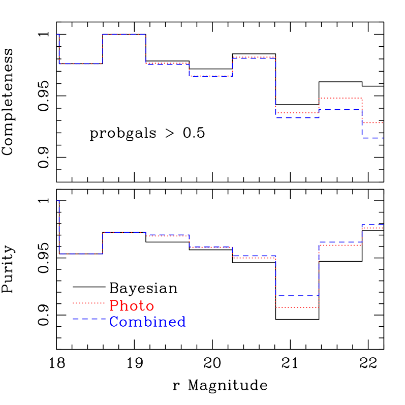
We conducted some simple tests to compare these classification schemes. If we set the Bayesian threshold to a value between 0.5 and 0.9, then both methods agree on the classification of more than of the objects for a random 1% subset of the SDSS photometric sample. We also tested the methods on a spectroscopic sample of 29,229 galaxies and stars (counting independent photometric measurements of each object) from the 2SLAQ and DEEP2 catalogs with . Defining stars as objects with , the sample contains 24,541 galaxies and 4,688 stars. We wish to compare this spectroscopic “truth table” with the photometric classification of the two methods and with a combined method that classifies an object as a galaxy if and only if both separators classify it as a galaxy. For the purposes of this test, we say that the Bayesian scheme classifies an object as a galaxy if . We define galaxy completeness as the ratio of correctly identified galaxies to the total number of galaxies in the spectroscopic sample. Purity is defined as the ratio of correctly identified galaxies to the number of objects identified (correctly or not) as galaxies by the classifier. The purity depends in part on the relative numbers of galaxies and stars in the spectroscopic sample.
Fig. 12 shows the completeness and purity of the resulting galaxy catalogs in bins of magnitude for this spectroscopic sample. Overall, the Bayesian separator and PHOTO TYPE produce similar results for galaxy purity and completeness. Moreover, the agreement between the two classification methods is quite good on an object-by-object basis. The Bayesian separator with probgals achieves slightly higher completeness and slightly lower purity. By varying the boundary, we could improve the purity of the Bayesian galaxy sample at the expense of degrading its completeness. We note that the best value of to use in defining a galaxy photometric sample depends on the scientific applications of the sample, i.e., on whether completeness or purity is the more important feature. In statistical applications, instead of defining a galaxy sample one can also choose to weight objects by their Bayesian probability (Scranton et al. 2002).
Based on this test, we conclude that the photometric sample for which we have estimated photo-z’s has better than 90% galaxy purity.
Appendix C Photometric Redshifts for SDSS DR5
An earlier version of the photo-z catalog, produced for SDSS Data Release 5 (DR5), is publicly available on the SDSS DR5 website (and is also called photoz2). The methods used to construct that photo-z catalog were similar to the ones employed here for DR6, but the latter incorporates a number of important improvements. Here we briefly outline the differences between the two. We strongly recommend use of the DR6 photo-z catalog instead of the DR5 catalog.
The photometric galaxy sample selection has improved from DR5 to DR6, because we used more stringent cuts in defining the DR6 sample. The DR6 sample selection is described above in Appendix A. The DR5 photometric galaxy sample selection required the cmodel and model magnitudes to lie in the ranges and , and also required the value of the smear polarizability (Sheldon et al. 2004) to be . Also, for DR5, star-galaxy separation used the Bayesian estimator (see Appendix B) with the value , while for DR6 we used PHOTO TYPE. The additional cuts used for the DR6 catalog have produced a cleaner and more reliable galaxy sample.
| No̱ of Galaxies | Object Description | |
|---|---|---|
| - | million | All |
| 0 | million | Complete & bright |
| 1 | million | Incomplete & bright |
| 2 | million | Complete & faint |
| 3 | million | Incomplete & faint |
Note. — The flag scheme for the DR5 catalog is based on object detection in some/all passbands and the magnitude. Incomplete objects are undetected in at least one of the passbands () and faint objects have .
| No̱ of Galaxies | Object Description | |
|---|---|---|
| - | million | All |
| 0 | million | bright |
| 2 | million | faint |
Note. — The scheme for the DR6 catalog is based solely on the on the magnitude: faint objects have .
The DR5 photo-z catalog included a number of flags describing the expected photo-z quality, shown in Table 4. These flags were based on the detection or non-detection of the object in all passbands and on the value of the model magnitude. An object was classified as bright (faint) if (). An object was flagged as “incomplete” if it was not detected in all five SDSS passbands. Table 4 shows the corresponding flag values and the number of objects assigned each flag value. For the DR6 sample, given the stricter sample selection, a very small number of objects would have been classified as incomplete by the definition above, and they have been removed from the sample. As a result, for DR6, we only supply the bright/faint flag, as shown in Table 5.
The spectroscopic training set used for the DR6 photo-z catalog has important additions compared to the one used for the DR5 catalog. In particular, for DR6 we added the DEEP2 spectroscopic catalog (which became publicly available), which made the training set more complete at faint magnitudes. We also implemented more stringent spectroscopic quality cuts to the training set used for DR6.
Unlike the DR5 training set, the DR6 training set does not contain objects from the SDSS “special” plates, extra spectroscopic observations designed to target specific objects for various scientific studies (Adelman-McCarthy et al. 2006). In our tests, we find that the lack of special plates does not result in any degradation of the photo-z quality.
The photo-z algorithm also changed from DR5 to DR6: we increased the number of hidden-layer nodes in the ANN and we added the concentration indices to the data inputs. Our tests indicated that this leads to improved photo-z performance according to our metrics. In addition, the CC2 method differs from DR5 photo-z’s further in that CC2 uses only the color information and not the raw magnitudes. For general purpose, full sample photo-z’s, we recommend using CC2 photo-z’s over both DR5 and D1 photo-z’s. Finally, we have carried out more extensive tests of the DR6 photo-z’s than were done for DR5, increasing our confidence in the robustness of the photo-z estimates.
References
- Abazajian et al. (2004) Abazajian, K. et al. 2004, AJ, 128, 502
- Adelman-McCarthy et al. (2006) Adelman-McCarthy, J. K. et al. 2006, ApJS, 162, 38
- Adelman-McCarthy et al. (2007a) —. 2007a, ApJS, in press
- Adelman-McCarthy et al. (2007b) —. 2007b, ApJS, submitted
- Bertin & Arnouts (1996) Bertin, E. & Arnouts, S. 1996, A&AS, 117, 393
- Blanton et al. (2003) Blanton, M. R., Lin, H., Lupton, R. H., Maley, F. M., Young, N., Zehavi, I., & Loveday, J. 2003, AJ, 125, 2276
- Cannon et al. (2006) Cannon, R. et al. 2006, MNRAS, 372, 425
- Coleman et al. (1980) Coleman, G. D., Wu, C. C., & Weedman, D. W. 1980, ApJS, 43, 393
- Collister & Lahav (2004) Collister, A. A. & Lahav, O. 2004, PASP, 116, 345
- Connolly et al. (1995) Connolly, A. J. et al. 1995, AJ, 110, 2655
- Csabai et al. (2003) Csabai, I. et al. 2003, AJ, 125, 580
- Csabai et al. (2007) —. 2007, in preparation
- Cunha et al. (2007) Cunha, C., Oyaizu, H., Lima, M., Lin, H., & Frieman, J. 2007, in preparation
- d’Abrusco et al. (2007) d’Abrusco, R. et al. 2007, ArXiv Astrophysics e-prints, 0701137
- Davis et al. (2001) Davis, M., Newman, J. A., Faber, S. M., & Phillips, A. C. 2001, in Deep Fields, ed. S. Cristiani, A. Renzini, & R. E. Williams, 241–+
- Eisenstein et al. (2001) Eisenstein, D. J. et al. 2001, AJ, 122, 2267
- Fukugita et al. (1996) Fukugita, M., Ichikawa, T., Gunn, J. E., Doi, M., Shimasaku, K., & Schneider, D. P. 1996, AJ, 111, 1748
- Gunn et al. (1998) Gunn, J. E. et al. 1998, AJ, 116, 3040
- Gunn et al. (2006) —. 2006, AJ, 131, 2332
- Hogg et al. (2001) Hogg, D. W., Finkbeiner, D. P., Schlegel, D. J., & Gunn, J. E. 2001, AJ, 122, 2129
- Ivezić et al. (2004) Ivezić, Ž. et al. 2004, Astronomische Nachrichten, 325, 583
- Lilly et al. (1995) Lilly, S. J., Le Fevre, O., Crampton, D., Hammer, F., & Tresse, L. 1995, ApJ, 455, 50
- Lima et al. (2007) Lima, M., Cunha, C., Oyaizu, H., Sheldon, E., Lin, H., & Frieman, J. 2007, in preparation
- Lupton et al. (2001) Lupton, R., Gunn, J. E., Ivezić, Z., Knapp, G. R., & Kent, S. 2001, in ASP Conf. Ser. 238: Astronomical Data Analysis Software and Systems X, ed. F. R. Harnden, Jr., F. A. Primini, & H. E. Payne, 269
- Morgan (1958) Morgan, W. W. 1958, PASP, 70, 364
- Oyaizu et al. (2007) Oyaizu, H., Lima, M., Cunha, C., Lin, H., & Frieman, J. 2007, in preparation
- Park & Choi (2005) Park, C. & Choi, Y.-Y. 2005, ApJ, 635, L29
- Pier et al. (2003) Pier, J. R. et al. 2003, AJ, 125, 1559
- Press et al. (1992) Press, W. H. et al. 1992, Numerical Recipes in C: The Art of Scientific Computing (Cambridge University Press)
- Schlegel et al. (1998) Schlegel, D. J., Finkbeiner, D. P., & Davis, M. 1998, ApJ, 500, 525
- Scranton et al. (2002) Scranton, R. et al. 2002, ApJ, 579, 48
- Sheldon et al. (2004) Sheldon, E. S. et al. 2004, AJ, 127, 2544
- Shimasaku et al. (2001) Shimasaku, K. et al. 2001, AJ, 122, 1238
- Smith et al. (2002) Smith, J. A. et al. 2002, AJ, 123, 2121
- Stoughton et al. (2002) Stoughton, C. et al. 2002, AJ, 123, 485
- Strauss et al. (2002) Strauss, M. A. et al. 2002, AJ, 124, 1810
- Tucker et al. (2006) Tucker, D. L. et al. 2006, Astronomische Nachrichten, 327, 821
- Vanzella et al. (2004) Vanzella, E. et al. 2004, A&A, 423, 761
- Wadadekar (2005) Wadadekar, Y. 2005, Publ. Astron. Soc. Pac., 117, 79
- Wang et al. (2007) Wang, D., Zhang, Y. X., Liu, C., & Zhao, Y. H. 2007, ArXiv e-prints, 07062704
- Weiner et al. (2005) Weiner, B. J. et al. 2005, ApJ, 620, 595
- Wirth et al. (2004) Wirth, G. D. et al. 2004, AJ, 127, 3121
- Yamauchi et al. (2005) Yamauchi, C. et al. 2005, AJ, 130, 1545
- Yee et al. (2000) Yee, H. K. C. et al. 2000, ApJS, 129, 475
- York et al. (2000) York, D. G. et al. 2000, AJ, 120, 1579