Lensing corrections to features in the angular two-point correlation function and power spectrum

Abstract

It is well known that magnification bias, the modulation of galaxy or quasar source counts by gravitational lensing, can change the observed angular correlation function. We investigate magnification-induced changes to the shape of the observed correlation function $w(\theta)$, and the angular power spectrum $C_{\ell}$, paying special attention to the matter-radiation equality peak and the baryon wiggles. Lensing effectively mixes the correlation function of the source galaxies with that of the matter correlation at the lower redshifts of the lenses distorting the observed correlation function. We quantify how the lensing corrections depend on the width of the selection function, the galaxy bias $b$, and the number count slope $s$. The lensing correction increases with redshift and larger corrections are present for sources with steep number count slopes and/or broad redshift distributions. The most drastic changes to $C_{\ell}$ occur for measurements at high redshifts ($z\mathrel{\hbox to0.0pt{\lower 4.0pt\hbox{\hskip 1.0pt$\sim$}\hss}\raise 1.0pt\hbox{$>$}}1.5$) and low multipole moment ($\ell\mathrel{\hbox to0.0pt{\lower 4.0pt\hbox{\hskip 1.0pt$\sim$}\hss}\raise 1.0pt\hbox{$<$}}100$). For the source distributions we consider, magnification bias can shift the location of the matter-radiation equality scale by $1$–$6\%$ at $z\sim 1.5$ and by $z\sim 3.5$ the shift can be as large as $30\%$. The baryon bump in $\theta^{2}w(\theta)$ is shifted by $\mathrel{\hbox to0.0pt{\lower 4.0pt\hbox{\hskip 1.0pt$\sim$}\hss}\raise 1.0pt\hbox{$<$}}1\%$ and the width is typically increased by $\sim 10\%$. Shifts of $\mathrel{\hbox to0.0pt{\lower 4.0pt\hbox{\hskip 1.0pt$\sim$}\hss}\raise 1.0pt\hbox{$>$}}0.5\%$ and broadening $\mathrel{\hbox to0.0pt{\lower 4.0pt\hbox{\hskip 1.0pt$\sim$}\hss}\raise 1.0pt\hbox{$>$}}20\%$ occur only for very broad selection functions and/or galaxies with $(5s-2)/b\mathrel{\hbox to0.0pt{\lower 4.0pt\hbox{\hskip 1.0pt$\sim$}\hss}\raise 1.0pt\hbox{$>$}}2$. However, near the baryon bump the magnification correction is not constant but is a gently varying function which depends on the source population. Depending on how the $w(\theta)$ data is fitted, this correction may need to be accounted for when using the baryon acoustic scale for precision cosmology.

I Introduction

The galaxy two-point angular correlation function and its spherical harmonic transform, the angular power spectrum, provide information about dark matter clustering. These statistics have scale dependent features which may be used as “standard rulers” to measure cosmological distances Peebles1973 ; Cooray06 . Features in the three-dimensional power spectrum which appear at a comoving wave number $k$ will appear in the angular power spectrum at redshift $z_{0}$ at multipole $\ell\sim k\chi(z_{0})$, where $\chi(z_{0})$ is the comoving distance to $z_{0}$. One such feature is the peak in the power spectrum that separates the modes which entered the horizon during radiation domination from those modes that entered during matter domination. This scale is determined by the horizon size at matter-radiation equality. Also present in the power spectrum are the so-called baryon acoustic oscillations (BAO). This series of wiggles in Fourier space is a signature of acoustic oscillations in the photon-baryon fluid that was present in the early universe. The location of the peaks of the BAO depends on the horizon size at the time of recombination BAO1 ; BAO2 ; BAO3 ; BAO4 ; BAO5 ; EH98 ; BAO6 . This scale is robustly measured from the cosmic microwave background WMAPI ; WMAPIII , and thus can serve as a “standard ruler”; given the scale of the BAO a measurement of the angular size of the BAO at some redshift will yield the angular diameter distance to that redshift . In fact the first measurements of this peak have occurred recently BAOmeas1 ; BAOmeas2 ; BAOmeas3 ; BAOmeas4 ; BAOmeas5 . In recent years, much effort has gone towards using these features in the correlation function for precision measurements BAOth1 .

Gravitational lensing changes the observed number density of galaxy or quasar sources - an effect called magnification bias Gunn67 ; Narayan1989 ; BTP1996 . (Hereafter, the terms ‘galaxy’ and ‘quasar’ can be considered synonymous.) It is well known that magnification bias modifies the galaxy angular correlation function Villumsen1995 ; VFC97 ; MJV98 ; MJ98 ; EGmag03 ; ScrantonSDSS05 ; menard ; JSS03 . In this paper we extend the previous analyses by investigating and quantifying how magnification bias changes the shape of the angular two point correlation function, and its spherical harmonic transform the angular power spectrum, paying special attention to important features such as the turnover in the power spectrum and the BAO.

Corrections from gravitational lensing enter as follows. The two-point function is measured from the galaxy number density fluctuation.

$$\delta_{n}=\frac{n({\bf x},z)-\bar{n}(z)}{\bar{n}(z)}$$ (1)

The effect of gravitational lensing is to alter the area of the patch of sky being observed and to change the observed flux of the source. Both effects change the measured galaxy number density, the first by changing the area, the second by changing the number of sources observed in a flux limited survey. Together these effects are called magnification bias Gunn67 ; Narayan1989 ; Villumsen1995 ; BTP1996 . To first order (i.e. the weak lensing limit), they lead to a correction term $\delta_{\mu}$ being added to the intrinsic galaxy fluctuation $\delta_{g}$

$$\delta_{n}=\delta_{g}+\delta_{\mu}$$ (2)

With this term the observed autocorrelation function becomes,

$$\langle\delta_{n}\delta_{n}\rangle=\langle\delta_{g}\delta_{g}\rangle+\langle\delta_{g}\delta_{\mu}\rangle+\langle\delta_{\mu}\delta_{g}\rangle+\langle\delta_{\mu}\delta_{\mu}\rangle.$$ (3)

The galaxy-galaxy term $\langle\delta_{g}\delta_{g}\rangle$ depends on the matter distribution at the source galaxies. The magnification terms, especially $\langle\delta_{\mu}\delta_{\mu}\rangle$, depend on the matter distribution spanning the range between the sources and the observer.

The lensing of high redshift quasars by low redshift galaxies have been detected confirming the presence of magnification bias for these systems. The most recent measurements of this effect are discussed in EGmag03 ; JSS03 ; ScrantonSDSS05 (see also Myers2003 ). Discussions of earlier measurements can be found in the references therein. These measurements work by cross-correlating the angular positions of galaxies/quasars at widely separated redshifts. Here, we will focus on the angular correlation of galaxies at similar redshifts. As was first pointed out by Matsubara , magnification bias alters observations of the 3D clustering of galaxies. In two separate papers 3Dpaper1 ; 3Dpaper2 , we further consider the effect of magnification bias on the 3D correlation function and power spectrum, which turn out to have qualitatively new and interesting features.

While this paper was in preparation, a paper addressing weak gravitational lensing corrections to baryon acoustic oscillations was posted otherpaper . In that paper they consider the effect of magnification bias (a first order correction) and stochastic deflection (a second order correction) on BAO in the real space correlation function for a delta function source distribution. In contrast, we consider the effect of magnification bias on the angular correlation function and the angular power spectrum for an extended source distribution. As we will show the width of the source distribution strongly affects the magnitude of the magnification bias correction. While some conclusions we reach are addressed in otherpaper , the observables considered and the analyses here are different.

This paper is organized as follows. In section II we present expressions for the angular auto-correlation function and the angular power spectrum when magnification bias is included. In section III we discuss the factors affecting the relative magnitude of the magnification bias terms compared with the galaxy term. In section IV we examine the effect of magnification on the shape of the angular power spectrum for a few different source distributions. In section V we consider the effect of magnification on the baryon bump in the angular correlation function. In VI we conclude and discuss the implications of our work for future surveys.

II Anisotropies and Correlation functions

We consider the two-dimensional galaxy fluctuation in direction $\hat{\mbox{\boldmath$\theta$}}$ integrated over a selection function with mean redshift $z_{0}$

$$\delta_{n}(\hat{\mbox{\boldmath$\theta$}},z_{0})=\frac{n(\hat{\mbox{\boldmath$\theta$}},z_{0})-\bar{n}(z_{0})}{\bar{n}(z_{0})}$$ (4)

where $\bar{n}$ is the mean number of galaxies in the redshift bin. We include this label, $z_{0}$, to remind the reader that the angular fluctuation depends on the source selection function.

When the effect of magnification bias is considered, the expression for the net measured galaxy overdensity becomes a sum of two terms (Equation 2). In the expressions that follow and throughout this paper we assume a flat universe, generalizing to an open or closed universe is fairly straightforward. The first term in Equation 2 is the intrinsic galaxy fluctuation integrated over a normalized selection function given by $W(z,z_{0})$,

$$\delta_{g}(\hat{\mbox{\boldmath$\theta$}},z_{0})=\int_{0}^{\infty}\!\!dz\,b(z)W(z,z_{0})\delta(\chi(z)\hat{\mbox{\boldmath$\theta$}},z).$$ (5)

Where $\chi(z)$ is the comoving distance to redshift $z$, $\delta=(\rho-\bar{\rho})/\bar{\rho}$ is the matter overdensity and $b(z)$ is a bias factor relating the galaxy number density fluctuation to the matter density fluctuation $\delta_{g}=b(z)\delta$. For simplicity we have assumed that the bias is scale independent, this should be accurate for $k\mathrel{\hbox to0.0pt{\lower 4.0pt\hbox{\hskip 1.0pt$\sim$}\hss}\raise 1.0pt\hbox{$<$}}0.05h\textrm{Mpc}^{-1}$, however at smaller scales it may be important (see for example RS3 ). If we further assume that $b(z)$ is slowly varying across $W(z,z_{0})$ then we can set $b(z)=b(z_{0})$ and pull it out of the integral in Equation 5.

The second term in Equation 2 is the correction due to magnification bias,

$$\delta_{\mu}(\hat{\mbox{\boldmath$\theta$}},z_{0})=\int_{0}^{\infty}\!\!dz\frac{c}{H(z)}\nabla_{\perp}^{2}\phi(\chi(z)\hat{\mbox{\boldmath$\theta$}},z_{0})\qquad\qquad\qquad$$ (6)

$$\times\,\,\chi(z)\int_{z}^{\infty}dz^{\prime}\left(5s(z^{\prime})-2\right)\frac{\chi(z^{\prime})-\chi(z)}{\chi(z^{\prime})}W(z^{\prime},z_{0}).$$

$H(z)$ is the Hubble parameter and $c$ is the speed of light Narayan1989 . The magnification bias term depends on the Laplacian of the gravitational potential $\phi$ (with respect to the comoving coordinates in the direction perpendicular to $\hat{\mbox{\boldmath$\theta$}}$) and the slope of the number count function. For a survey with limiting magnitude $m$ this is

$$s=\frac{d\textrm{log}_{10}N(<m)}{dm}.$$ (7)

If $s(z)$ is slowly varying across $W(z,z_{0})$, then we can set $s(z)=s(z_{0})$ and the expression for $\delta_{\mu}$ becomes

$$\delta_{\mu}(\hat{\mbox{\boldmath$\theta$}},z_{0}) = \left(5s(z_{0})-2\right)$$ (8)

$$\times \int_{0}^{\infty}\!\!dz\frac{c}{H(z)}g(z,z_{0})\nabla_{\perp}^{2}\phi(\chi(z)\hat{\mbox{\boldmath$\theta$}},z_{0}).$$

Where we have introduced the lensing weight function

$$g(z,z_{0})=\chi(z)\int_{z}^{\infty}dz^{\prime}\frac{\chi(z^{\prime})-\chi(z)}{\chi(z^{\prime})}W(z^{\prime},z_{0}).$$ (9)

The lensing weight function can be thought of as roughly proportional to the probability for sources in $W(z,z_{0})$ to be lensed by density perturbations at $z$. The lensing weight function increases in magnitude as $z_{0}$ increases and is peaked at a redshift $z$ corresponding to about half the comoving distance to $z_{0}$.

On scales $k\gg aH$ Poisson’s equation can be used to relate the gravitational potential to the matter fluctuation

$$-k^{2}\phi({\bf k},z)=\frac{3H_{0}^{2}}{2c^{2}}\Omega_{m}(1+z)\delta({\bf k},z)$$ (10)

where ${\bf k}$ is the comoving wave vector, $k$ is its magnitude and $\Omega_{m}$ is the matter density today dodelson . .

We consider the two-point correlation function of the galaxy overdensity

$$w_{nn}(\theta,z_{0}) = \langle\delta_{g}(\hat{\mbox{\boldmath$\theta$}},z_{0})\delta_{g}(\hat{\mbox{\boldmath$\theta$}}^{\prime},z_{0})\rangle+2\langle\delta_{g}(\hat{\mbox{\boldmath$\theta$}},z_{0})\delta_{\mu}(\hat{\mbox{\boldmath$\theta$}}^{\prime},z_{0})\rangle$$ (11)

$$+ \langle\delta_{\mu}(\hat{\mbox{\boldmath$\theta$}},z_{0})\delta_{\mu}(\hat{\mbox{\boldmath$\theta$}}^{\prime},z_{0})\rangle$$

$$\equiv w_{gg}(\theta,z_{0})+2w_{g\mu}(\theta,z_{0})+w_{\mu\mu}(\theta,z_{0})$$

where $\cos\theta=\hat{\mbox{\boldmath$\theta$}}\cdot\hat{\mbox{\boldmath$\theta$}}^{\prime}$. In what follows we will consider the Legendre coefficients of the correlation functions. These are defined as

$$w_{gg}(\theta,z_{0})=\sum_{\ell}\frac{2\ell+1}{4\pi}C^{gg}_{\ell}(z_{0})P_{\ell}(\cos\theta)$$ (12)

where $P_{\ell}(\cos\theta)$ are the Legendre polynomials. The Legendre components of the observed correlation function, $w_{nn}(\theta,z_{0})$ will of course be a sum of all the terms,

$$C^{nn}_{\ell}(z_{0})=C^{gg}_{\ell}(z_{0})+2C^{g\mu}_{\ell}(z_{0})+C^{\mu\mu}_{\ell}(z_{0})$$ (13)

We calculate the angular power spectra, $C^{gg}_{\ell}$, $C^{g\mu}_{\ell}$ and $C^{\mu\mu}_{\ell}$, using the Limber approximation Limber which is accurate for $\ell\mathrel{\hbox to0.0pt{\lower 4.0pt\hbox{\hskip 1.0pt$\sim$}\hss}\raise 1.0pt\hbox{$>$}}10$. To simplify the expressions and provide some insight into the effects of the magnification terms we introduce the following functions

$$\phi^{gg}(z,z_{0})=b(z_{0})^{2}W(z,z_{0})^{2}\,\qquad\qquad\qquad\qquad\qquad\quad\,\,$$ (14)

$$\phi^{\mu\mu}(z,z_{0})=\qquad\qquad\qquad\qquad\qquad\qquad\qquad\qquad\qquad\,$$ (15)

$$\frac{9}{4}(5s(z_{0})-2)^{2}\Omega^{2}_{m}\frac{H_{0}^{4}}{c^{2}H(z)^{2}}g^{2}(z,z_{0})(1+z)^{2}$$

$$\phi^{g\mu}(z,z_{0})=\sqrt{\phi^{gg}(z,z_{0})\phi^{\mu\mu}(z,z_{0})}\qquad\qquad\qquad\qquad\quad$$ (16)

With this notation the angular correlation functions can all be expressed as

$$C^{xx}_{\ell}(z_{0})=\int_{0}^{\infty}\frac{dz}{\chi(z)^{2}}\frac{H(z)}{c}\phi^{xx}(z,z_{0})P\left(\frac{\ell}{\chi(z)},z\right)$$ (17)

where $xx$ symbolizes $gg$, $g\mu$ or $\mu\mu$ and $P(k=\ell/\chi(z),z)$ is the matter power spectrum.

Figure 1: The redshift distributions normalized by the galaxy bias (Eq. 14-15), $\phi^{gg}/b^{2}$ (dashed line), $2\phi^{g\mu}/b^{2}$ (dot-dashed line) and $\phi^{\mu\mu}/b^{2}$ (dotted line) shown here for Gaussian selection functions centered at $z_{0}=1.5$ and $z_{0}=2.5$ with $\sigma=0.15$. These distributions determine the angular power spectra through Equation 17. The total auto-correlation $C^{nn}_{\ell}/b^{2}$ will depend on $(\phi^{gg}+2\phi^{g\mu}+\phi^{\mu\mu})/b^{2}$ (solid line).

For illustration we use Gaussian selection functions

$$W(z,z_{0})=\frac{1}{\sqrt{2\pi}\sigma}\textrm{exp}\left[-\frac{(z-z_{0})^{2}}{2\sigma^{2}}\right]$$ (18)

of various widths to demonstrate how the shape of the selection function alters the effect of magnification.

We assume a flat $\Lambda$CDM cosmology with $\Omega_{m}=0.27$, $\Omega_{\Lambda}=0.73$ and $\Omega_{b}=0.0224/h^{2}$ as the fractional energy densities in matter, vacuum and baryons today. The Hubble constant $H_{0}=100h$ km/s/Mpc is set to $h=0.7$, the fluctuation amplitude to $\sigma_{8}=0.8$, and scalar spectral index $n_{s}=0.95$. For the linear power spectrum we use the Eisenstein and Hu transfer function EH98 . In a few places (e.g. Figure 2) we discuss the no-BAO spectrum, this is calculated using the BBKS transfer function BBKS with a modified shape parameter $\Gamma=\Omega_{m}h\,\textrm{exp}[-\Omega_{b}(1+\sqrt{2h}/\Omega_{m})]$ GammaSugiyama . The non-linear evolution of both power spectra is calculated using the prescription of Smith et. al. Smithetal . The nonlinear power spectrum is used in all plots and discussions.

Unless otherwise stated we set the galaxy sample dependent ratio $(5s-2)/b=1$ (see mepaper ; 3Dpaper1 on how this varies with galaxy sample and redshift). The first correction term, $C^{g\mu}_{\ell}/b^{2}$ is linear in this quantity while the second term, $C^{\mu\mu}_{\ell}/b^{2}$ is quadratic. Thus the magnitude of the net correction, calculated here cannot in general be scaled by $(5s-2)/b$. However, at low redshifts $2C^{g\mu}_{\ell}/b^{2}$ dominates over $C^{\mu\mu}_{\ell}/b^{2}$ and at higher redshifts $C^{\mu\mu}_{\ell}>2C^{g\mu}_{\ell}$. The redshift of the transition between the two regimes increases with the width of the selection function. Specifically when $\sigma=0.07$, $2C^{g\mu}_{\ell}<C^{\mu\mu}_{\ell}$ for $z_{0}\geq 1.5$, when $\sigma=0.15$, $2C^{g\mu}_{\ell}<C^{\mu\mu}_{\ell}$ for $z_{0}\geq 2.0$ and when $\sigma=0.30$, $2C^{g\mu}_{\ell}<C^{\mu\mu}_{\ell}$ for $z_{0}\geq 2.5$.

III amplitude of the lensing corrections

The relative magnitude of the lensing magnification terms, $C^{g\mu}_{\ell}$ and $C^{\mu\mu}_{\ell}$, to the intrinsic galaxy term, $C^{gg}_{\ell}$, depends on several things: first the galaxy-sample dependent quantities $b$ and $s$, and second the selection function and cosmological quantities in Equations 14–15. Here we discuss how these quantities affect the relative magnitudes of $C^{gg}_{\ell}$, $C^{g\mu}_{\ell}$ and $C^{\mu\mu}_{\ell}$.

The magnification terms are scaled by the galaxy-sample dependent factors $(5s-2)/b$ and $(5s-2)^{2}/b^{2}$. Thus for a given galaxy bias, galaxies residing on the steep end of the luminosity function will have larger magnification corrections. However, if $s<2/5$, the galaxy-magnification term $C^{g\mu}_{\ell}$ is negative, while the magnification-magnification term, $C^{\mu\mu}_{\ell}$ is always positive. Unless otherwise stated we fix $(5s-2)/b=1$ so both terms are positive.

The difference between the galaxy-galaxy, galaxy-magnification and magnification-magnification terms can be seen more clearly by considering equations 14–17. From Equation 17, we see that all the angular power spectra are simply integrals of the power spectrum over some redshift distribution $\phi^{xx}(z,z_{0})$. Examples of these distributions for a selection function with $\sigma=0.15$ are shown in Figure 1. In the case of $\phi^{gg}(z,z_{0})$ this distribution is determined by the selection function. This suggests that one can think of the magnification terms as adding to $C^{gg}_{\ell}$ measurements of the correlation function with “selection functions” determined by $\phi^{g\mu}(z,z_{0})$ and $\phi^{\mu\mu}(z,z_{0})$.

Figure 1 shows that $\phi^{g\mu}(z,z_{0})$ is peaked not too far from where the selection function is peaked, and is similar in shape to the selection function. Thus we expect $C^{g\mu}_{\ell}$ to be similar in shape to $C^{gg}_{\ell}$. On the other hand, the magnification-magnification term $\phi^{\mu\mu}$ is peaked at a much lower redshift than the selection function and is also much more broadly distributed in redshift. Thus we expect $C^{\mu\mu}_{\ell}$ to be peaked at lower $\ell$ (larger angular scales) than $C^{gg}_{\ell}$ because it is probing structure at lower redshifts which is nearer to the observer and occupies a larger angle in the sky. Additionally, since $\phi^{\mu\mu}(z,z_{0})$ is rather broadly distributed, we expect sharp features such as baryon oscillations to be smoothed out in $C^{\mu\mu}_{\ell}$.

One might infer from looking at Figure 1 that the magnification bias terms $C^{g\mu}_{\ell}$ and $C^{\mu\mu}_{\ell}$ will be quite small compared to $C^{gg}_{\ell}$. However, the other quantities in the integrand of Equation 17 decrease with redshift so the relative magnitudes of $\phi^{gg}$, $\phi^{g\mu}$ and $\phi^{\mu\mu}$ do not completely determine the relative magnitudes of $C^{gg}_{\ell}$,$C^{g\mu}_{\ell}$ and $C^{\mu\mu}_{\ell}$.

IV the shape of the Angular power spectrum

Figure 2: The angular power spectra divided by the no-BAO power spectra for a selection function of width $\sigma=0.15$. The dashed line is $C^{gg}_{\ell}$ alone (no magnification case), the solid line is $C^{nn}_{\ell}=C^{gg}_{\ell}+2C^{g\mu}_{\ell}+C^{\mu\mu}_{\ell}$.

Using equations 14–15 and 17 we calculate the angular power spectra using Gaussian selection functions centered at a variety of redshifts. Because the galaxy-magnification cross term $C^{g\mu}_{\ell}$ depends strongly on the width of the selection function, we consider several different widths given by $\sigma=0.07,0.15,0.30$. The magnification-magnification term $C^{\mu\mu}_{\ell}$ is largely independent of the width of the selection function, but the galaxy-magnification term $C^{g\mu}_{\ell}$ increases with increasing width of the selection function. The effect of increasing $\sigma$ is therefore to increase the overall contribution of magnification to $C^{nn}_{\ell}$.

In Figure 2 we show the angular power spectrum with and without magnification bias for a selection function of width $\sigma=0.15$. In this figure the power spectra are normalized by the no-BAO power spectrum, which is calculated neglecting magnification bias and the effects of baryons. We see immediately several features: the effect of magnification is largest at the low $\ell$ values (small $\ell$ correspond to large angular scales), the magnitude of the magnification correction increases with redshift, and the effect at high $\ell$ near the baryon wiggles is mostly (though not completely) to boost the amplitude rather than change the shape of the spectrum.

Magnification clearly changes the shape of the angular power spectrum. The most significant changes are at $\ell\mathrel{\hbox to0.0pt{\lower 4.0pt\hbox{\hskip 1.0pt$\sim$}\hss}\raise 1.0pt\hbox{$<$}}100$ where the peak in the power spectrum resides. The peak in the power spectrum is an important feature because its location is related to the Hubble scale when the universe transitions from radiation domination to matter domination. This feature in the power spectrum can be used as a standard ruler Cooray06 .

We identify the location $\ell_{peak}$ and amplitude of the peak in $C^{gg}_{\ell}$ and $C^{nn}_{\ell}$. The shift in $\ell_{peak}$, and the fractional change in amplitude, $(C^{nn}_{\ell}-C^{gg}_{\ell})/C^{gg}_{\ell}$ (where $C^{nn}_{\ell}$ is evaluated at the $\ell_{peak}$ for $C^{nn}_{\ell}$ and $C^{gg}_{\ell}$ is evaluated at the $\ell_{peak}$ found for $C^{gg}_{\ell}$) when magnification is included are shown in Table 1. The change in $\ell_{peak}$ and the change in amplitude increase both with redshift and with increasing width of the selection function $\sigma$. The value of $\ell_{peak}$ is also dependent on the width of the selection function, with $\ell_{peak}$ taking slightly larger values for narrower selection functions.

One additional consequence of magnification bias is to change the redshift and scale at which non-linear evolution of the power spectrum becomes important. This is because even for sources at high redshift where non-linearity is small, $C^{\mu\mu}_{\ell}$ will depend on structure at low redshift where non-linearity is important. Indeed, even at $z_{0}=3.5$ the difference between $C^{nn}_{\ell}$ calculated with the non-linear power spectrum and $C^{nn}_{\ell}$ calculated with the linear power spectrum is $\mathrel{\hbox to0.0pt{\lower 4.0pt\hbox{\hskip 1.0pt$\sim$}\hss}\raise 1.0pt\hbox{$>$}}10\%$ by $\ell\sim 1800,1400,1000$ for $\sigma=0.07$, $0.15$ and $0.30$ respectively. This is to be compared with $C^{gg}_{\ell}$, the no magnification case, for which the difference between $C^{gg}_{\ell}(z_{0}=3.5)$ calculated with and without non-linear evolution does not approach $10\%$ until $\ell\sim 2600$ for each value of $\sigma$.

	$\sigma=0.07$			$\sigma=0.15$			$\sigma=0.30$
$z_{0}$	$\ell_{peak}$	$\Delta\ell_{peak}$	$\Delta C_{\ell_{peak}}/C^{gg}_{\ell_{peak}}$	$\ell_{peak}$	$\Delta\ell_{peak}$	$\Delta C_{\ell_{peak}}/C^{gg}_{\ell_{peak}}$	$\ell_{peak}$	$\Delta\ell_{peak}$	$\Delta C_{\ell_{peak}}/C^{gg}_{\ell_{peak}}$
$0.5$	$19$	$0$	$0.02$	$16$	$0$	$0.04$	$-$	$-$	$-$
$1.0$	$34$	$0$	$0.01$	$33$	$0$	$0.04$	$30$	$-2$	$0.14$
$1.5$	$46$	$-1$	$0.02$	$45$	$-1$	$0.05$	$44$	$-3$	$0.14$
$2.0$	$55$	$-1$	$0.03$	$54$	$-3$	$0.07$	$54$	$-5$	$0.17$
$2.5$	$62$	$-2$	$0.04$	$61$	$-5$	$0.10$	$61$	$-9$	$0.22$
$3.0$	$67$	$-3$	$0.06$	$67$	$-8$	$0.13$	$67$	$-15$	$0.29$
$3.5$	$72$	$-5$	$0.08$	$72$	$-11$	$0.17$	$72$	$-21$	$0.38$

Table 1: A table of quantities related to the matter-radiation equality peak for a variety of mean redshifts $z_{0}$ and selection function widths $\sigma$. The peak location (of $C^{gg}_{\ell}$) is $\ell_{peak}$, the shift in the peak location when magnification is included is $\Delta\ell_{peak}=\ell_{peak}^{nn}-\ell_{peak}^{gg}$, and the change in height at the peak is $\Delta C_{\ell_{peak}}/C_{\ell_{peak}}=\left(C^{nn}_{\ell_{peak}}-C^{gg}_{\ell_{peak}}\right)/C^{gg}_{\ell_{peak}}$. For $z_{0}=0.5$, we do not consider the case of a wide selection function $\sigma=0.30$.

V the angular correlation function and the baryon bump

We now turn our attention to the real space angular correlation function $w_{nn}(\theta,z_{0})$ (Equation 11). In multipole space, the baryon oscillations appear as a series of peaks in the power spectrum (e.g. Figure 2). In real space the signature of baryon oscillations is a single bump in the correlation function. The location of the bump in $w_{nn}(\theta,z_{0})$ is determined by the comoving sound horizon at recombination and the distance to $z_{0}$. The sound horizon at recombination is measured quite precisely from the cosmic microwave background anisotropy, thus a measurement of $\theta_{BAO}$ at $z_{0}$ can give a measure of the comoving distance to $z_{0}$.

Before we address the lensing corrections to the baryon bump, we will first discuss a few issues that arise (whether or not lensing is included) when using the angular correlation function to measure the baryon oscillation scale. The angular correlation function is in some sense averaging the matter power spectrum across different redshifts. Thus, if too broad of a selection function is used the baryon feature will be washed out. For a fixed width in redshift, the washing out is more severe at low redshifts because $\Delta\chi\sim\Delta z/H(z)$ and $H(z)$ decreases with decreasing $z$. Additionally, the baryon bump is a subtle feature in the angular correlation function. It is customary to multiply the angular correlation function by $\theta^{2}$ to make the baryon bump easier to identify and characterize. Indeed for the cases we have considered this is necessary in order for there to be a local maximum at the acoustic scale at all. Figure 3 illustrates this point: while there is a baryon feature, there is no local maximum in $w(\theta)$. In Figure 4 we show $\theta^{2}w(\theta)$ in the region near the baryon bump, in this case the baryon feature is quite visible for $\sigma=0.07$ but is very hard to identify for $\sigma=0.30$, fortunately the baryon bump becomes more prominent with increasing redshift.

Since the baryon bump is broadened at low redshifts we limit our analysis to $z_{0}\geq 1.0$ for $\sigma=0.07$ and $0.15$ and $z_{0}\geq 2.0$ for $\sigma=0.30$. We have experimented with multiplying by $\theta^{3}$: in this case even for the broadest selection function $\sigma=0.30$ the baryon bump is visible at all redshifts we consider. Interestingly, the magnitude of the shift in the baryon oscillation scale due to magnification bias is sensitive to whether one looks at $\theta^{2}w(\theta)$ or $\theta^{3}w(\theta)$. The shift is much larger in the latter case, suggesting that the importance of magnification bias for baryon oscillation measurements depends on precisely how the baryon bump is fitted. In this paper, we focus on the effects on $\theta^{2}w(\theta)$.

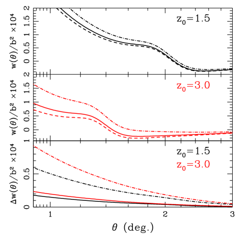
Figure 3: Top and middle panels: the two-point function divided by the galaxy bias $w(\theta)/b^{2}$. This is using a selection function of width $\sigma=0.15$ centered at $z_{0}=1.5$ (top) and ${}_{0}=3.0$ (middle). The dashed line neglects magnification, the solid line includes magnification with $(5s-2)/b=1$, the dot-dashed line includes magnification with $(5s-2)/b=2$. Bottom panel: the magnification correction, $(w_{nn}(\theta)-w_{gg}(\theta))/b^{2}$. The solid line is for $(5s-2)/b=1$, the dot-dashed line is for $(5s-2)/b=2$

Figure 4: Here we zoom in on baryon bump in $\theta^{2}w(\theta)/b^{2}$ at $z_{0}=1.5$. The dashed lines neglect magnification $\theta^{2}w_{gg}(\theta)/b^{2}$ the solid lines include magnification $\theta^{2}w_{nn}(\theta)/b^{2}$. The broader the selection function, the harder it is to locate the baryon peak, the presence of magnification bias doesn’t change this.

We calculate the two-point function $w_{nn}(\theta,z_{0})$ by performing the sum in Equation 12. In Figure 3 we plot $w_{nn}(\theta)$ and $w_{gg}(\theta)$ with redshift bins centered at $z_{0}=1.5$ and $z_{0}=3.0$ for a small angular range near the baryon bump. One can see from Figure 3 that, as expected, the angular correlation function is changed by magnification bias.

The lensing correction to the angular correlation function is scale dependent. To address how the baryon bump is changed by lensing magnification we consider the location of the baryon peak $\theta_{BAO}$, the height at the peak $\theta^{2}w(\theta_{BAO})$, and the peak width. The peak width is defined to be $\left[\left(\frac{\partial^{2}}{d\theta^{2}}\theta^{2}w\right)/(\theta^{2}w)\right]^{-1/2}$ evaluated at $\theta_{BAO}$.

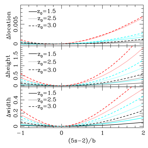
Figure 5: Effects of magnification bias on the baryon bump as found in $\theta^{2}w(\theta)$. Shown here for selection functions with $\sigma=0.07$ (black lowest curves), $\sigma=0.15$ (cyan middle curves), and $\sigma=0.30$ (red upper curves) as a function of the galaxy population-dependent ratio $(5s-2)/b$ for several different mean redshifts. Upper panel: the fractional change in the angular location of the baryon bump $(\theta_{BAO}^{nn}-\theta_{BAO}^{gg})/\theta_{BAO}^{gg}$. Middle panel: the fractional change in the height of the baryon bump, $(w_{nn}(\theta^{nn}_{BAO})-w_{gg}(\theta^{gg}_{BAO}))/w_{gg}(\theta_{BAO}^{gg})$. Bottom panel: the fractional change of the width of the baryon bump – see text for how the width is defined.

Figure 5 summarizes the fractional changes in the peak location, height and width as a function of $(5s-2)/b$ for selection functions with $\sigma=0.07$, $0.15$ and $0.30$, and for several redshifts. The magnitude of the changes to the peak increase with redshift for all $\sigma$. The changes in peak location and width are largest at the highest redshifts ($z_{0}=3-3.5$) but the exact redshift dependence varies depending on the selection function. This is in part because broader selection functions grant a larger $w_{g\mu}(\theta)$ term which dominates at low redshifts. In the region near the baryon bump, this term is more strongly scale dependent than $w_{\mu\mu}(\theta)$. Additionally, the baryon peak is sharper and the amplitude of $w_{gg}(\theta)$ is larger for narrower selection functions (e.g. Figure 4), both of these factors make it more difficult for magnification to effect the peak location.

Magnification shifts $\theta_{BAO}$ by $<0.5\%$ for all $\sigma$ and $z_{0}$ values we considered. The changes to the width and amplitude are much larger. We should point out that as the width of the selection function is increased the baryon bump is also broadened making the peak harder to identify – this is true regardless of whether magnification bias is present. This is illustrated in Figure 4, where we show $\theta^{2}w(\theta)$ for a narrow angular range for each $\sigma$. One can see that for $\sigma=0.30$ there is no maximum at this redshift.

We have shown that the change in location of the baryon bump found in our calculated $w_{nn}(\theta)$ and $w_{gg}(\theta)$ is likely to be small. However, an actual measurement of $\theta_{BAO}$ will involve fitting a curve to data points with error bars. From this perspective, magnification bias – which adds a scale and source population dependent correction to $w_{gg}(\theta)$ – may be of more concern. This fact is illustrated in the lower panel of Figure 3. Here we show the difference between the two-point functions with and without magnification ($w_{nn}-w_{gg}$). Although this difference is slowly varying in the region around the baryon peak, the value of the difference is not constant. In the regime very near the peak the offset between $w_{nn}(\theta)$ and $w_{gg}(\theta)$ can be approximated as a straight line. The precise slope of this line will depend on the population of galaxies via $b$ and $s$. Interestingly, the magnification correction to $\theta^{2}w(\theta)$ is closer to a constant than it is for $w(\theta)$. When the baryon bump in $\theta^{3}w(\theta)$ is considered we find the magnification correction is more strongly scale dependent than for $\theta^{2}w(\theta)$. Thus the changes to the baryon peak location in $\theta^{3}w(\theta)$ are significantly larger (by a factor of $5-6$). We emphasize then, that while Figure 5 gives an indication of the effect of magnification bias on the baryon bump, the actual effect of magnification on measurements of the acoustic scale will depend on the method by which the peak location is fitted from the data. When using the BAO peak as a standard ruler this scale and population dependent bias should be taken into account.

VI discussion

The angular two-point correlation function and the angular power spectrum are important cosmological statistics, but a complete understanding of systematics is necessary to use these to derive precise constraints on cosmological parameters. Magnification bias, a gravitational lensing correction to the observed number density of sources, has been known to change the correlation function at high redshifts Villumsen1995 ; VFC97 ; MJV98 ; MJ98 . We have examined and quantified how magnification bias changes the shape of the angular correlation function and power spectrum. The effect of magnification is to adjust both the scale-dependence and amplitude of the correlation function. We have shown that the scale-dependence changes the location of the matter-radiation equality peak in the angular power spectrum, and can potentially lead to a bias in determining the location of the baryon bump in the angular correlation function (see Figures 2, 3, 5 and Table 1). Magnification bias becomes important at high redshifts ($z\mathrel{\hbox to0.0pt{\lower 4.0pt\hbox{\hskip 1.0pt$\sim$}\hss}\raise 1.0pt\hbox{$>$}}1.5$) with the most drastic scale dependent changes occurring at low multipoles $\ell\mathrel{\hbox to0.0pt{\lower 4.0pt\hbox{\hskip 1.0pt$\sim$}\hss}\raise 1.0pt\hbox{$<$}}100$. Precisely how, if ignored, magnification would bias measurements of the matter-radiation equality scale or the BAO size will likely depend on how these quantities are extracted from the correlation function as well as the population of galaxies or quasars used for the measurement. Finally, the magnification terms are sensitive to non-linear evolution of structure at low redshifts even for sources at high redshift. Consequently, the presence of magnification bias changes the redshift and scale for which non-linear evolution of the power spectrum is visible.

Magnification bias is a source-population dependent effect, that is the magnitude (and even the sign) of the correction depend on the population of galaxies or quasars being observed. On the one hand, one may be able to select a population of sources with number count slope $s=2/5$, in which case magnification bias vanishes. However, such a selection may reduce the number of sources available for analysis so this is not necessarily the best option. Current measurements of the galaxy angular correlation are at redshifts $z<1$, so the correction from magnification to these observations is expected to be negligible. Projections for measurements of galaxy clustering from future high redshift galaxy surveys will need to address the effect of magnification bias.

Finally, let us reiterate that this paper focuses exclusively on the angular correlation. The effect of magnification bias on the 3D correlation has some surprising new features. For instance, in certain situations, magnification bias can be important even for low redshift measurements. This was originally noted by Matsubara and is further analyzed in two separate papers 3Dpaper1 ; 3Dpaper2 .

- (1) P. J. E. Peebles, Astrophys. J. 185, 413 (1973); M. G. Hauser, P. J. E. Peebles Astrophys. J. 185, 757 (1973); E. J. Groth, P. J. E. Peebles Astrophys. J. 217, 385 (1977); M. Tegmark Phys. Rev. Lett. 79, 3806 (1997); M. Tegmark, A. J. S. Hamilton, M. A. Strauss, M. S. Vogeley, A. S. Szalay Astrophys. J. 499, 555 (1998); Y. Wang, D. N. Spergel, M. A. Strauss Astrophys. J. 510, 20 (1999); W. Hu, D. J. Eisenstein, M. Tegmark, M. White Phys. Rev. D59, 023512 (1998); D. J. Eisenstein, W. Hu, M. Tegmark, Astrophys. J. 518, 2 (1999)
- (2) A. Cooray, Astrophys. J. 651, L77 (2006)
- (3) J. Silk, Astrophys. J. 151, 459 (1968)
- (4) P. J. E. Peebles, J. T. Yu, Astrophys. J. 162, 815 (1970)
- (5) R. A. Sunyeav, Ya. B. Zel’dovich, Astrophysics and Space Science, 7, 3S (1970)
- (6) J. R. Bond, G. Efstathiou, Astrophys. J. 285, 45 (1984)
- (7) J. A. Holtzman, Astrophys. J. Suppl. 7, 1 (,) 1 (1989)
- (8) Eisenstein, D. J., Hu, W., Astrophys. J. 496, 605 (1998)
- (9) A. Meiksin, M. White, J. A. Peacock Mon. Not. R. Astron. Soc. 304, 851 (1999)
- (10) D. Spergel et al.Astrophys. J. Suppl.148, 175 (2003)
- (11) D. Spergel et al., Astrophys. J. , in press
- (12) D. J. Eisenstein, W. Hu, M. Tegmark Astrophys. J. 504, 57 (1998); H.- J. Seo, D. J. Eisenstein Astrophys. J. 598, 720 (2003); E. V. Linder, Phys. Rev. D68, 083504 (2003); T. Matsubara, A. S. Szalay, Phys. Rev. Lett. 90, 021302 (2003); C. Blake, K. Glazebrook Astrophys. J. 594, 655 (2003); W. Hu, Z. Haiman, Phys. Rev. D68, 063004 (2003); T. Matsubara Astrophys. J. 615, 573 (2004); H.- J. Seo, D. J. Eisenstein Astrophys. J. 633, 575 (2005); K. Glazebrook, C. Blake Astrophys. J. 631, 1 (2005); M. White, Astropart. Phys., 24, 334 (2005); C. Blake, S. Bridle, Mon. Not. R. Astron. Soc. 363, 1329 (2005); R. Angulo, C.M. Baugh, C.S. Frenk, R. G. Bower, A. Jenkins, S. L. Morris Mon. Not. R. Astron. Soc. 262, L25 (2005); C. Blake, D. Parkinson, B. Basset, K. Glazebrook, M. Kunz, R. C. Nichol Mon. Not. R. Astron. Soc. 365, 255 (2006); D. Dolney, B. Jain, M. Takada Mon. Not. R. Astron. Soc. 366, 884 (2006); D. Dolney, B. Jain, M. Takada Mon. Not. R. Astron. Soc. 366, 884 (2006); D. Jeong, E. Komatsu, Astrophys. J. 651, 619 (2006); E. Huff, A. E. Schulz, M. White, D. Schlegel, M. S. Warren, Astropart. Phys. 26, 351 (2007); R. Angulo, C. M. Baugh, C. S. Frenk, C. G. Lacey Mon. Not. R. Astron. Soc. in press (2007)
- (13) S. Cole, et al., Mon. Not. R. Astron. Soc. 362, 505 (2005)
- (14) D. J. Eisenstein, et al.Astrophys. J. 633,560 (2005)
- (15) G. Huetsi, Astron. & Astrophys. submitted (2005) astro-ph
- (16) N. Padmanabhan, et al.Mon. Not. R. Astron. Soc. submitted (2006) astro-ph
- (17) W. Percival, et al.Astrophys. J. 657, 51 (2007)
- (18) J. E. Gunn, Astrophys. J. 147 61 (1967)
- (19) E. L. Turner, J. P. Ostriker, J. R. Gott, Astrophys. J. 284, 1 (1984); R. L. Webster, P. C. Hewett, M. E. Harding, G. A. Wegner, Nature 336, 358 (1988); W. Fugmann, Astron. & Astrophys. 204, 73 (1988); R. Narayan, Astrophys. J. Lett. 339, 53 (1989); P. Schneider, Astron. & Astrophys. 221, 221 (1989).
- (20) T. J. Broadhurst, A. N. Taylor, J. A. Peacock, Astrophys. J. 438, 49 (1996)
- (21) J. V. Villumsen, unpublished preprint (1995) astro-ph
- (22) J. Villumsen, W. Freudling, L. N. da Costa, Astrophys. J. 481, 578 (1997)
- (23) R. Moessner, B. Jain, J. Villumsen, Mon. Not. R. Astron. Soc. 294, 291 (1998)
- (24) R. Moessner, B. Jain,Mon. Not. R. Astron. Soc. 294, L18 (1998)
- (25) E. Gaztañaga, Astrophys. J. 589, 82 (2003)
- (26) R. Scranton, et al., Astrophys. J. 633, 589 (2005)
- (27) A. D. Myers, et al.Mon. Not. R. Astron. Soc. 342, 467 (2003)
- (28) B. Menard, M. Bartelmann, Astron. & Astrophys. 386, 784 (2002).
- (29) B. Jain, R. Scranton, R. V. Sheth, Mon. Not. R. Astron. Soc. 345, 62 (2003)
- (30) T. Matsubara, Astrophys. J. 537, L77 (2000)
- (31) L. Hui, E. Gaztanaga, M. LoVerde, submitted to Phys. Rev. D(2007) arxiv
- (32) L. Hui, E. Gaztanaga, M. LoVerde, submitted to Phys. Rev. D(2007b) arxiv
- (33) A. Vallinotto, S. Dodelson, C. Schimd, J. P. Uzan (2007) astro-ph
- (34) For a review, see S. Dodelson, Modern Cosmology, Academic Press (2003).
- (35) R. E. Smith, R. Scoccimarro, R. K. Sheth, Phys. Rev. D75, 063512 (2007)
- (36) D. N. Limber, Astrophys. J. 119, 655 (1954)
- (37) J. M. Bardeen, J. R. Bond, N. Kaiser, A. S. Szalay, Astrophys. J. 304, 15B (1986)
- (38) N. Sugiyama, Astrophys. J. Suppl. 1, 0 (0) , 281 (1995)
- (39) R. E. Smith, et al.Mon. Not. R. Astron. Soc. 341 1311 (2003)
- (40) M. LoVerde, L. Hui, E. Gaztañaga, Phys. Rev. D75, 043519 (2007)