Collective modes of $CP^{3}$ Skyrmion crystals in quantum Hall ferromagnets

Abstract

The two-dimensional electron gas (2DEG) in a bilayer quantum Hall system can sustain an interlayer coherence at filling factor $\nu=1$ even in the absence of tunneling between the layers. This system, which can be described as a quantum Hall pseudospin ferromagnet, has low-energy charged excitations which may carry textures in real spin or pseudospin. Away from filling factor $\nu=1,$ a finite density of these is present in the ground state of the 2DEG and forms a crystal. Depending on the relative size of the various energy scales, such as tunneling ($\Delta_{SAS}$), Zeeman coupling ($\Delta_{Z}$) or electrical bias ($\Delta_{b}$), these textured crystal states can involve spin, pseudospin, or both intertwined. This last case is a “CP³ Skyrmion Crystal”. In this article, we present a comprehensive numerical study of the collective excitations of these textured crystals using the Generalized Random-Phase Approximation. For the pure spin case, at finite Zeeman coupling the state is a Skyrmion crystal with a gapless phonon mode, and a separate Goldstone mode that arises from a broken $U\left(1\right)$ symmetry. At zero Zeeman coupling, we demonstrate that the constituent Skyrmions break up, and the resulting state is a meron crystal with four gapless modes. In contrast, a pure pseudospin Skyrme crystal at finite tunneling has only the phonon mode. For $\Delta_{SAS}\rightarrow 0,$ the state evolves into a meron crystal and supports an extra gapless ($U(1)$) mode in addition to the phonon. For a $CP^{3}$ Skyrmion crystal, we find a $U(1)$ gapless mode in the presence of non-vanishing symmetry-breaking fields $\Delta_{SAS}$, $\Delta_{Z},$ and $\Delta_{b}$. In addition, a second mode with a very small gap is present in the spectrum. We present dispersion relations for the different low-energy modes of these various crystals as well as their physical interpretations.

I Introduction

The two-dimensional electron gas (2DEG) in a bilayer quantum Hall system has a broken-symmetry ground state at filling factor $\nu=1$ that can be described as a pseudospin ferromagnet. This state is characterized by finite interlayer coherence even in the absence of tunneling. Interlayer coherence is maintained if the interlayer separation $d$ is lower than a critical separation which is of the order of $d_{c}\approx 1.25\ell$ at zero electrical bias where $\ell=\sqrt{\hslash c/eB}$ is the magnetic length. This state has been extensively studied, both experimentally and theoretically (for a review, see Ref. review, ). Its collective excitationfertigdispersion , which has been detected experimentallyspielmanpseudospinmode , is a pseudospin wave mode in which the pseudospins precess around their equilibrium orientations.

In most studies of the interlayer coherent states at $\nu=1$ or at other filling factors where states such as Wigner crystals, Skyrmion crystals or bilayer stripes are predicted, it is assumed that the 2DEG is spin polarized so that the non-interacting 2DEG can be mapped onto a two-level system with bonding and anti-bonding states. Recent experimentskumadaprl ; spielmanprl , however, cast some doubt on the validity of this assumption. To explain these recent experimental findings, it seems that the ground state should be partially spin depolarized.

A previous studycotecp3 (which we refer to as Paper I in the rest of this article) presented various zero-temperature phases of the 2DEG in a bilayer quantum Hall system when the filling factor is varied around $\nu=1$, so that a finite density of charged excitations is introduced in the ground state. Working in the Hartree-Fock approximation, various symmetry breaking fields were present in the system: tunnelling $\left(\Delta_{SAS}\right)$, Zeeman $\left(\Delta_{Z}\right)$ and electrical bias $\left(\Delta_{b}\right)$, over a range of experimentally relevant filling factors ($0.6\leq\nu\leq 1.2$) and interlayer separations ($0\leq d/\ell\lesssim 1.0$). The phase diagram depends sensitively on the interplay of the different symmetry breaking fields as well as filling factor and interlayer separation. In some regions of the phase diagram, the 2DEG is pseudospin polarized and the charged excitations are Skyrmions with real spin texture (i.e., spin-Skyrmions) while in regions where the Zeeman coupling dominates, the 2DEG is spin-polarized and the charged excitations are Skyrmions with pseudospin texture (i.e., pseudospin Skyrmions or bimerons.) The phase diagram contains also some regions where the charged excitations involve intertwined spin and pseudospin textures. These complex objects are called $CP^{3}$ Skyrmionsrajaramancp3 . Spin and pseudospin-Skyrmions can be viewed as limiting cases of the more general $CP^{3}$ Skyrmion excitation.

In the present paper, our main goal is to understand the collective mode spectrum of a crystal of $CP^{3}$ Skyrmions. To understand the intricate spectrum of excitations in such a crystal, we find it helpful to begin our study by calculations of the collective mode spectra of pure spin or pseudospin Skyrmion crystals as well as that of the homogeneous (or liquid) state at exactly $\nu=1$.

For the liquid state, an analysis of the collective excitations was presented in Ref. hasebe, , but the analysis was limited to the behavior at long wavelengths. We provide here the full dispersion relations, calculated in the Generalized Random-Phase Approximation (GRPA), of the three Goldstone modes identified in Ref. hasebe, . In addition to pseudospin-wave and spin-wave modes, the $CP^{3}$ liquid state also supports a gapless mode involving a spin and a pseudospin flip.

The collective mode spectrum of a pure spin-Skyrmion crystal was first calculated in Ref.cotegirvinprl, . In this work we present and discuss both two-component cases: the spin and pseudospin crystals, and discuss the similarities and differences. The spin-Skyrmion has two Goldstone modes at finite Zeeman coupling. One is the phonon mode which is due to the broken translational symmetry, while the second mode is a $U\left(1\right)$ phase mode arising from a broken orientational symmetry in the spin texture. Indeed, the energy of an isolated spin-Skyrmion is invariant with respect to a global change in the azimuthal angle of the spins. In a crystal, this angle is fixed and this symmetry is broken. It is believedcotegirvinprl that this mode is responsible for the small NMR relaxation time $T_{1}$ observed experimentallybarret around $\nu=1$ at low temperature. A particularly interesting situation arises if one considers the limit of vanishing Zeeman coupling $\Delta_{Z}$: each Skyrmion breaks up into two merons (a meron is a vortex-like configuration which can be understood as half a Skyrmion), and the resulting meron crystal has $three$ Goldstone modes in addition to the phonon mode which are similar in nature to the $U\left(1\right)$ phase mode of the spin-Skyrmion crystal.

For the analogous bilayer situation, where the two layers in which the electrons may reside play the role of the two allowed spin states, we find that only the phonon mode remains gapless in the pseudospin-Skyrmion crystal when the tunneling and layer separation are both non-vanishing. The absence of a gapless mode analogous to the $U(1)$ mode of the spin-Skyrmion crystal occurs because the inter-layer interaction is different than the intra-layer interaction, breaking the $U(1)$ symmetry. For $\Delta_{SAS}\rightarrow 0$, the state deforms into a pseudospin meron crystal, which has two (rather than four) gapless modes because of the explicit symmetry-breaking in the interaction. These modes may be identified as a phonon, and a Goldstone mode due to the spontaneous interlayer coherence in the limit of zero tunneling and the broken orientational symmetry in the in-plane pseudospin texture.

For the $CP^{3}$ Skyrmion crystal, we show that, when all symmetry breaking fields $\Delta_{SAS}$, $\Delta_{Z},$ and $\Delta_{b}$ are finite, the crystal has, in addition to the phonon mode, one gapless phase $U\left(1\right)$ mode arising from the invariance of the Hamiltonian with respect to a rotation of all the spins in the two layers by the same angle. We find also that since the $CP^{3}$ Skyrmion crystal occurs only at very small value of the tunneling parameter, a second phase mode with a very small gap is present in the spectrum. Our $CP^{3}$ Skyrmion crystal is characterized by a set of eight low-energy modes that offer a distinct signature of this entangled spin and pseudospin state, much different from that of a pure spin or pseudospin Skyrmion crystal.

Our paper is organized in the following way. We introduce our description of the crystal phases in the bilayer quantum Hall system in Sec. II and the formalism we use to compute the dispersion relations of the collective modes in the GRPA in Sec. III. We study the collective mode spectrum of the liquid state for $\nu=1$ in Sec. IV, that of the pure spin-Skyrmion crystal in Sec. V, and that of the pure pseudospin crystal in Sec. VI. We are then ready in Sec. VII to consider the more general case of a $CP^{3}$ Skyrmion crystal. We study the excitation spectrum of this crystal as a function of interlayer separation, tunnel coupling and electrical bias. Finally, we conclude in Sec. VIII.

II Description of the crystal states

We consider a 2DEG in a double-quantum-well system (DQWS) in a quantizing magnetic field $\mathbf{B}=B\widehat{\mathbf{z}}$ taking into account the possibility that an electrical bias is applied to the system. We define this bias as $\Delta_{b}=E_{R}-E_{L}$ where $E_{R\left(L\right)}$ are the electric subband energies in each well (right and left) in the absence of magnetic field and tunneling. For simplicity, we make a narrow well approximation, i.e. we assume that the width $b$ of the wells is small ($b<<\ell$ ) and treat interlayer hopping in a tight-binding approximation. The single-particle problem is then characterized by the total filling factor $\nu$, the separation $d$ (from center to center) between the wells, the tunneling gap $\Delta_{SAS}$, the electrical bias $\Delta_{b}$ and the Zeeman energy $\Delta_{Z}=g^{\ast}\mu_{B}B$ where $g^{\ast}$ is the effective gyromagnetic factor and $\mu_{B}$ is the Bohr magneton.

We describe the phases of the electrons in the DQWS by the set of average fields $\left\{\left\langle\rho_{i,j}^{\alpha,\beta}(\mathbf{q})\right\rangle\right\}$ where $\rho_{i,j}^{\alpha,\beta}(\mathbf{q})$ is an operator that we definecotemethode as

$$\rho_{i,j}^{\alpha,\beta}(\mathbf{q})=\frac{1}{N_{\varphi}}\sum_{X}e^{-iq_{x}X+iq_{x}q_{y}\ell^{2}/2}\ c_{i,\alpha,X}^{\dagger}c_{j,\beta,X-q_{y}\ell^{2}}.$$ (1)

In this equation, $N_{\varphi}=S/2\pi\ell^{2}$ is the Landau level degeneracy with $S$ the area of the 2DEG. The indices $i,j=R,L$ and $\alpha,\beta=\pm 1$ are respectively well and spin indices. We use the Landau gauge with vector potential $\mathbf{A}=\left(0,Bx,0\right)$. The operator $c_{i,\alpha,X}^{\dagger}$ creates an electron in state $\left(i,\alpha,X\right)$ in the lowest Landau level. We work in the strong magnetic field limit where the Hilbert space is restricted to the lowest Landau level only and make the usual approximation of neglecting Landau level mixing. For a crystal state, only the fields $\left\langle\rho_{i,j}^{\alpha,\beta}(\mathbf{q=G})\right\rangle\mathbf{\neq 0,}$ where $\mathbf{G}$ is a reciprocal lattice vector of the crystal structure. The calculation of the order parameters $\left\langle\rho_{i,j}^{\alpha,\beta}(\mathbf{q=G})\right\rangle$ in the Hartree-Fock approximation for a crystal of $CP^{3}$ Skyrmions was explained in Paper Icotecp3 .

The Hartree-Fock Hamiltonian of a general crystal state is given by

$$H_{HF} = N_{\phi}\sum_{i,\alpha}\widetilde{E}_{\alpha,i}\rho_{i,i}^{\alpha,\alpha}\left(0\right)$$

$$-N_{\phi}\frac{\Delta_{SAS}}{2}\sum_{\alpha}\left(\rho_{R,L}^{\alpha,\alpha}\left(0\right)+\rho_{L,R}^{\alpha,\alpha}\left(0\right)\right)$$

$$+N_{\phi}\sum_{\alpha,\beta}\sum_{i,j}\sum_{\mathbf{G}}H_{i,j}\left(G\right)\left\langle\rho_{i,i}^{\alpha,\alpha}(-\mathbf{G})\right\rangle\rho_{j,j}^{\beta,\beta}(\mathbf{G})$$

$$-N_{\phi}\sum_{\alpha,\beta}\sum_{i,j}\sum_{\mathbf{G}}X_{i,j}\left(G\right)\left\langle\rho_{i,j}^{\alpha,\beta}(-\mathbf{G})\right\rangle\rho_{j,i}^{\beta,\alpha}(\mathbf{G}),$$

with the renormalized single-particle energies given by

$$\widetilde{E}_{R,\alpha} = \frac{\Delta_{b}}{2}-\alpha\frac{\Delta_{Z}}{2}+\left(\frac{e^{2}}{\kappa\ell}\right)\left(\frac{\nu}{2}-\nu_{L}\right)\left(\frac{d}{\ell}\right),$$ (3)

$$\widetilde{E}_{L,\alpha} = -\frac{\Delta_{b}}{2}-\alpha\frac{\Delta_{Z}}{2}+\left(\frac{e^{2}}{\kappa\ell}\right)\left(\frac{\nu}{2}-\nu_{R}\right)\left(\frac{d}{\ell}\right),$$ (4)

and the Hartree and Fock intrawell and interwell interactions defined by

$$H_{i,i}\left(q\right) = H\left(q\right)=\left(\frac{e^{2}}{\kappa\ell}\right)\frac{1}{q\ell}e^{-q^{2}\ell^{2}}[1-\delta_{q,0}],$$ (5)

$$H_{i\neq j}\left(q\right) = \widetilde{H}\left(q\right)=\left(\frac{e^{2}}{\kappa\ell}\right)\frac{1}{q\ell}e^{-q^{2}\ell^{2}}[e^{-qd}-\delta_{q,0}],$$ (6)

$$X_{i,i}\left(q\right) = X\left(q\right)=\left(\frac{e^{2}}{\kappa\ell}\right)\int_{0}^{+\infty}dye^{-y^{2}/2}J_{0}\left(q\ell y\right),$$ (7)

$$X_{i\neq j}\left(q\right) = \widetilde{X}\left(q\right)$$

$$= \left(\frac{e^{2}}{\kappa\ell}\right)\int_{0}^{+\infty}dye^{-y^{2}/2}e^{-dy/\ell}J_{0}\left(q\ell y\right).$$

Note that to take into account a uniform neutralizing positive background, one sets $H\left(0\right)=0$ and $\widetilde{H}\left(0\right)=-\left(\frac{e^{2}}{\kappa\ell}\right)\frac{d}{\ell}.$

For the full four-level system, an electronic state may be specified by the four-component spinor

$$c_{X}=\left(\begin{array}[]{c}c_{R,+,X}\\ c_{R,-,X}\\ c_{L,+,X}\\ c_{L,-,X}\end{array}\right).$$ (9)

At this point, it is convenient to redefine the operators $\rho_{i,j}^{\alpha,\beta}(\mathbf{q})$ introduced above as $\rho_{a,b}(\mathbf{q})$ with the indices $a,b$ taking the four values $a,b=1,2,3,4$ and referring to the states $\left(R,+\right),(R,-),(L,+),(L,-)$ in this order. The layer index can be mapped into a pseudospin index $\pm_{p}$with the correspondance $R\rightarrow+_{p}$ and $L\rightarrow-_{p}$. The density, spin density, and pseudospin density operators $\rho\left(\mathbf{q}\right),\mathbf{S}\left(\mathbf{q}\right)$ and $\mathbf{P}\left(\mathbf{q}\right)$ and the nine operators $R_{u,v}\left(\mathbf{q}\right)$ (with $u,v=x,y,z$) are relatedezawasu4 to the four-component spinor of Eq. (9) by the equationscorrection

$$\rho(\mathbf{q})=\frac{1}{N_{\varphi}}\sum_{X}e^{-iq_{x}X+iq_{x}q_{y}\ell^{2}/2}\ c_{X}^{\dagger}c_{X-q_{y}\ell^{2}},$$ (10)

$$S_{u}(\mathbf{q})=\frac{1}{2N_{\varphi}}\sum_{X}e^{-iq_{x}X+iq_{x}q_{y}\ell^{2}/2}\ c_{X}^{\dagger}\tau_{u}^{spin}c_{X-q_{y}\ell^{2}},$$ (11)

$$P_{u}(\mathbf{q})=\frac{1}{2N_{\varphi}}\sum_{X}e^{-iq_{x}X+iq_{x}q_{y}\ell^{2}/2}\ c_{X}^{\dagger}\tau_{u}^{ppin}c_{X-q_{y}\ell^{2}},$$ (12)

$$R_{u,v}(\mathbf{q})=\frac{1}{2N_{\varphi}}\sum_{X}e^{-iq_{x}X+iq_{x}q_{y}\ell^{2}/2}\ c_{X}^{\dagger}\tau_{u}^{spin}\tau_{v}^{ppin}c_{X-q_{y}\ell^{2}},$$ (13)

where the $4\times 4$ matrices $\tau_{u}^{spin}$ and $\tau_{v}^{ppin}$ are defined by

$$\tau_{u}^{spin}=\left(\begin{array}[]{cc}\sigma_{u}&0\\ 0&\sigma_{u}\end{array}\right),$$ (14)

(with $\sigma_{u}$ a Pauli matrix) and by

$$\tau_{x}^{ppin}=\left(\begin{array}[]{cc}0&I\\ I&0\end{array}\right),\tau_{y}^{ppin}=\left(\begin{array}[]{cc}0&-iI\\ iI&0\end{array}\right),$$ (15)

and

$$\tau_{z}^{ppin}=\left(\begin{array}[]{cc}I&0\\ 0&-I\end{array}\right),$$ (16)

where $I$ is the $2\times 2$ unit matrix.

One may showcotecp3 that the order parameters obey the four sum rules

$$\sum_{\mathbf{G}}\sum_{b}\left|\left\langle\rho_{a,b}(\mathbf{G})\right\rangle\right|^{2}=\nu_{a}.$$ (17)

III Calculation of the response functions

We define the two-particle Matsubara Green’s functions as

$$\chi_{a,b,c,d}\left(\mathbf{q},\mathbf{q}^{\prime};\tau\right)=-N_{\phi}\left\langle T_{\tau}\delta\rho_{a,b}\left(\mathbf{q,}\tau\right)\delta\rho_{c,d}\left(\mathbf{-q}^{\prime},0\right)\right\rangle,$$ (18)

where $T_{\tau}$ is the imaginary time ordering operator. In a crystal, these functions are non zero only for wavectors $\mathbf{q=k+G}$ and $\mathbf{q}^{\prime}\mathbf{=k+G}^{\prime}$ where $\mathbf{k}$ is a vector in the first Brillouin zone of the lattice. The collective mode spectrum is found by tracking the poles of the response functions $\chi_{a,b,c,d}\left(\mathbf{k+G},\mathbf{k+G};i\Omega_{n}\rightarrow\omega+i\delta\right)$ when $\mathbf{k}$ varies in the Brillouin zone.

Let us denote by $a_{l},a_{s}$ the layer and spin indices in $a$ and similarly for the other indices $b,c,d$. The equations of motion for the two-particle Matsubara Green’s functions in the Hartree-Fock approximation (i.e. $\chi_{a,b,c,d}^{0}$) are given by

$$\hslash\frac{\partial}{\partial\tau}\chi_{a,b,c,d}^{0}\left(\mathbf{q},\mathbf{q}^{\prime};\tau\right)$$

$$= -N_{\varphi}\hslash\left\langle\left[\rho_{a,b}\left(\mathbf{q,}\tau\right),\rho_{c,d}\left(\mathbf{-q}^{\prime},0\right)\right]\right\rangle\delta\left(\tau\right)$$

$$-N_{\varphi}\left\langle T_{\tau}\left[H_{HF}-\mu N,\rho_{a,b}\left(\mathbf{q,}\tau\right)\right],\delta\rho_{c,d}\left(\mathbf{-q}^{\prime},0\right)\right\rangle,$$

with $H_{HF}$ given in Eq. (II). Evaluating the commutators and Fourier transforming with respect to the imaginary time $\tau$, we get the lengthy equation

$$\left[i\hslash\Omega_{n}+\left(\widetilde{E}_{a}-\widetilde{E}_{b}\right)\right]\chi_{a,b,c,d}^{0}\left(\mathbf{q},\mathbf{q}^{\prime};\Omega_{n}\right)$$

$$= \hslash\left\langle\rho_{a,d}\left(\mathbf{q-q}^{\prime}\right)\right\rangle\delta_{b,c}\gamma_{\mathbf{q},\mathbf{q}^{\prime}}$$

$$-\hslash\left\langle\rho_{c,b}\left(\mathbf{q-q}^{\prime}\right)\right\rangle\delta_{a,d}\gamma_{\mathbf{q},\mathbf{q}^{\prime}}^{\ast}$$

$$+\frac{1}{2}\Delta_{SAS}\delta_{a_{l},L}\chi_{\left(a_{s},R\right),b,c,d}^{0}\left(\mathbf{q},\mathbf{q}^{\prime};\Omega_{n}\right)$$

$$-\frac{1}{2}\Delta_{SAS}\delta_{b_{l},R}\chi_{a,\left(b_{s},L\right),c,d}^{0}\left(\mathbf{q},\mathbf{q}^{\prime};\Omega_{n}\right)$$

$$+\frac{1}{2}\Delta_{SAS}\delta_{a_{l},R}\chi_{\left(a_{s},L\right),b,c,d}^{0}\left(\mathbf{q},\mathbf{q}^{\prime};\Omega_{n}\right)$$

$$-\frac{1}{2}\Delta_{SAS}\delta_{b_{l},L}\chi_{a,\left(b_{s},R\right),c,d}^{0}\left(\mathbf{q},\mathbf{q}^{\prime};\Omega_{n}\right)$$

$$-\sum_{a^{\prime}}\sum_{\mathbf{q}^{\prime\prime}\neq\mathbf{q}}U_{a^{\prime},a}^{H}\left(\mathbf{q-q}^{\prime\prime}\right)\gamma_{\mathbf{q},\mathbf{q}^{\prime\prime}}\chi_{a,b,c,d}^{0}\left(\mathbf{q}^{\prime\prime},\mathbf{q}^{\prime};\Omega_{n}\right)$$

$$+\sum_{a^{\prime}}\sum_{\mathbf{q}^{\prime\prime}\neq\mathbf{q}}U_{a^{\prime},b}^{H}\left(\mathbf{q-q}^{\prime\prime}\right)\gamma_{\mathbf{q},\mathbf{q}^{\prime\prime}}^{\ast}\chi_{a,b,c,d}^{0}\left(\mathbf{q}^{\prime\prime},\mathbf{q}^{\prime};\Omega_{n}\right)$$

$$+\sum_{b^{\prime}}\sum_{\mathbf{q}^{\prime\prime}}U_{a,b^{\prime}}^{F}\left(\mathbf{q-q}^{\prime\prime}\right)\gamma_{\mathbf{q},\mathbf{q}^{\prime\prime}}\chi_{b^{\prime},b,c,d}^{0}\left(\mathbf{q}^{\prime\prime},\mathbf{q}^{\prime};\Omega_{n}\right)$$

$$-\sum_{a^{\prime}}\sum_{\mathbf{q}^{\prime\prime}}U_{a^{\prime},b}^{F}\left(\mathbf{q-q}^{\prime\prime}\right)\gamma_{\mathbf{q},\mathbf{q}^{\prime\prime}}^{\ast}\chi_{a,a^{\prime}c,d}^{0}\left(\mathbf{q}^{\prime\prime},\mathbf{q}^{\prime};\Omega_{n}\right),$$

where $\gamma_{\mathbf{q},\mathbf{q}^{\prime}}=e^{i\left(\mathbf{q}\times\mathbf{q}^{\prime}\right)\cdot\widehat{\mathbf{z}}\ell^{2}/2}$ and we have defined the mean-field Hartree and Fock potentials

$$U_{a,d}^{H}\left(\mathbf{q}\right) = H_{a_{l},d_{l}}\left(\mathbf{q}\right)\left\langle\rho^{a,a}\left(\mathbf{q}\right)\right\rangle,$$ (21)

$$U_{a,d}^{F}\left(\mathbf{q}\right) = X_{a_{l},d_{l}}\left(\mathbf{q}\right)\left\langle\rho^{a,d}\left(\mathbf{q}\right)\right\rangle,$$ (22)

with the Hartree and Fock interactions defined in Eqs. (5-II).

We get the response functions in the GRPA by summing the ladder and bubble diagramscotemethode . The result is the integral equation

$$\chi_{a,b,c,d}\left(\mathbf{q},\mathbf{q}^{\prime};\Omega_{n}\right)$$ (23)

$$=\chi_{a,b,c,d}^{0}\left(\mathbf{q},\mathbf{q}^{\prime};\Omega_{n}\right)$$

$$+\frac{1}{\hslash}\sum_{\mathbf{q}^{\prime\prime}}\chi_{a,b,e,e}^{0}\left(\mathbf{q},\mathbf{q}^{\prime\prime};\Omega_{n}\right)H_{e,g}\left(\mathbf{q}^{\prime\prime}\right)\chi_{g,g,c,d}\left(\mathbf{q}^{\prime\prime},\mathbf{q}^{\prime};\Omega_{n}\right)$$

$$-\frac{1}{\hslash}\sum_{\mathbf{q}^{\prime\prime}}\chi_{a,b,e,f}^{0}\left(\mathbf{q},\mathbf{q}^{\prime\prime};\Omega_{n}\right)X_{e,f}\left(\mathbf{q}^{\prime\prime}\right)\chi_{f,e,c,d}\left(\mathbf{q}^{\prime\prime},\mathbf{q}^{\prime};\Omega_{n}\right).$$

We now write Eq. (23) in a matrix form more appropriate for numerical analysis. We first redefine $\chi_{a,b,c,d}$ as the matrix $\chi_{i,j}$ with the indices $i,j$ taking the values from $1$ to $16$ with the order: $(1,1),(1,2),(1,3),(1,4),(2,1),$etc. for $i,$ the row index, and the order: $(1,1),(2,1),(3,1),(4,1),(1,2),$ etc. for $j$, the column index. It is to be noted that all elements $\chi_{i,j}$ of the matrix $\chi$ as well as of the other matrices $I,A,B,H,X$ that we define below are themselves matrices in the reciprocal lattice vectors $\mathbf{G},\mathbf{G}^{\prime}.$ In the end, we have to diagonalize a matrix with dimensions $16n_{RLV}\times 16n_{RLV}$ where $n_{RLV}$ is the number of reciprocal lattice vectors $\mathbf{G}$ that we keep in the calculation. We typically work with $n_{RLV}\approx 317$ (in the calculation of the order parameters, however, we keep more than $600$ reciprocal lattice vectors). We then write the index $i$ as $i=4\left(\overline{i}-1\right)+\widetilde{i}$ where $\overline{i},\widetilde{i}=1,2,3,4$ and similarly for $j$. The unit matrix is written as

$$I=\delta_{\overline{i},\overline{j}}\delta_{\widetilde{i},\widetilde{j}}\delta_{\mathbf{q,q}^{\prime}}.$$ (24)

We define the following matrices:

$$B_{i,j}\left(\mathbf{q},\mathbf{q}^{\prime}\right) = \left\langle\rho_{\overline{i},\overline{j}}\left(\mathbf{q-q}^{\prime}\right)\right\rangle\gamma_{\mathbf{q},\mathbf{q}^{\prime}}\delta_{\widetilde{i},\widetilde{j}}$$

$$-\left\langle\rho_{\widetilde{j},\widetilde{i}}\left(\mathbf{q-q}^{\prime}\right)\right\rangle\gamma_{\mathbf{q},\mathbf{q}^{\prime}}^{\ast}\delta_{\overline{i},\overline{j}},$$

$$E_{i,j}\left(\mathbf{q},\mathbf{q}^{\prime}\right)=-\left(\widetilde{E}_{\overline{i}}-\widetilde{E}_{\widetilde{i}}\right)\delta_{i,j}\delta_{\mathbf{q,q}^{\prime}},$$ (26)

$$F_{i,j}\left(\mathbf{q},\mathbf{q}^{\prime}\right) = -\left(H_{\overline{i}}^{+}\left(\mathbf{q},\mathbf{q}^{\prime}\right)-H_{\widetilde{i}}^{-}\left(\mathbf{q},\mathbf{q}^{\prime}\right)\right)\delta_{i,j}$$

$$+F_{\overline{i},\overline{j}}^{+}\left(\mathbf{q},\mathbf{q}^{\prime}\right)\delta_{\widetilde{i},\widetilde{j}}-F_{\widetilde{j},\widetilde{i}}^{-}\left(\mathbf{q},\mathbf{q}^{\prime}\right)\delta_{\overline{i},\overline{j}},$$

$$T_{i,j}\left(\mathbf{q},\mathbf{q}^{\prime}\right) = \frac{\Delta_{SAS}}{2}\delta_{\overline{i},\overline{j}}\delta_{\left|\widetilde{i}-\widetilde{j}\right|,2}\delta_{\mathbf{q,q}^{\prime}},$$

$$-\frac{\Delta_{SAS}}{2}\delta_{\widetilde{i},\widetilde{j}}\delta_{\left|\overline{i}-\overline{j}\right|,2}\delta_{\mathbf{q,q}^{\prime}}$$

with the definitions (with $k,l=1,2,3,4$)

$$H_{k}^{\pm}\left(\mathbf{q},\mathbf{q}^{\prime}\right)=\sum_{a^{\prime}}U_{a^{\prime},k}^{H}\left(\mathbf{q-q}^{\prime}\right)e^{\pm i\left(\mathbf{q}\times\mathbf{q}^{\prime\prime}\right)\cdot\widehat{\mathbf{z}}\ell^{2}/2},$$ (29)

and

$$F_{k,l}^{\pm}\left(\mathbf{q-q}^{\prime\prime}\right)=U_{k,l}^{F}\left(\mathbf{q-q}^{\prime}\right)e^{\pm i\left(\mathbf{q}\times\mathbf{q}^{\prime\prime}\right)\cdot\widehat{\mathbf{z}}\ell^{2}/2}.$$

We also define the interactions

$$V_{i,j}\left(\mathbf{q},\mathbf{q}^{\prime}\right)=\left[H_{\overline{i},\overline{j}}\left(\mathbf{q}\right)\delta_{\widetilde{i},\overline{i}}\delta_{\widetilde{j},\overline{j}}-X_{\widetilde{j},\overline{j}}\left(\mathbf{q}\right)\delta_{i,j}\right]\delta_{\mathbf{q,q}^{\prime}}.$$ (30)

With all these definitions, we can write the equation of motion for the response functions in the matrix form:

$$\left[i\hslash\Omega_{n}I-E-T-F-BV\right]\chi=\hslash B.$$ (31)

To get the weight of each pole, we diagonalize the matrix $M=E+T+F+BV$ by writing $MU=UD$ where $U$ is the matrix containing the eigenvectors and $D$ is the diagonal matrix of the eigenvalues $\hslash\omega_{j}\left(\mathbf{k}\right)$. The response function $\chi$ can be written as

$$\chi_{n,m}\left(\mathbf{k},\omega\right)=\sum_{j,k}\frac{U_{n,j}\left(\mathbf{k}\right)\left[U\left(\mathbf{k}\right)\right]_{j,k}^{-1}B_{k,m}\left(\mathbf{k}\right)}{\omega+i\delta-\omega_{j}\left(\mathbf{k}\right)}$$ (32)

where the indices $n,m,j,k=1,2,...,16n_{RLV}.$ Using Eqs. (10-13), it is easy to get from $\chi$ the response functions for the density, spin, pseudospin and the $R$ fields. Because we have access to the matrix of eigenvectors $U$, we can also animate the motion of the density, spin, pseudospin, etc. in a given mode. This will be very helpful for the interpretation of the different modes.

IV Uniform coherent state at $\nu=1$

In this section, we apply our formalism to the study of the spin-polarized uniform coherent state (UCS) at $\nu=1$. For effectively spinless electrons, the behavior of the collective mode (i.e. pseudospin wave) with bias and interlayer separation was studied before in Ref. joglekar, . One may also considerhasebe the limit of an $SU(4)\$ symmetric Hamiltonian, in which the interlayer separation $d$, $\Delta_{Z}$, and $\Delta_{SAS}$ are all set to zero. In this case three Goldstone modes were predicted in the absence of symmetry-breaking fieldshasebe using a gradient expansion, but quantitative dispersion relations for these modes that takes into account the spin, pseudospin and density fields are difficult to obtain in this approach. Our GRPA formalism produces these three modes, provides analytical results for the dispersions in some limiting cases, and allows numerical results to be obtained in the general case from the microscopic Hamiltonian.

In UCS, the only non-zero order parameters are

$$\left\langle\rho_{1,1}\left(0\right)\right\rangle = \nu_{1},$$

$$\left\langle\rho_{3,3}\left(0\right)\right\rangle = \nu_{3},$$ (33)

$$\left\langle\rho_{1,3}\left(0\right)\right\rangle = \left|\left\langle\rho_{3,1}\left(0\right)\right\rangle\right|^{\ast}=\alpha,$$

(we can choose $\alpha$ real without lost of generality). For a balanced DQWS, $\nu_{1}=\nu_{3}$ while in the presence of a bias, $\nu_{1},\nu_{3}$ and $\alpha$ must be found by minimizing the Hartree-Fock energy. We have discussed the effect of a bias on the UCS in Paper Icotecp3 . In the absence of tunneling, we obtain a simple relation between charge imbalance and bias,

$$\sigma=\nu_{3}-\nu_{1}=\frac{-\Delta_{b}}{X\left(0\right)-\widetilde{X}\left(0\right)-\frac{d}{\ell}\left(\frac{e^{2}}{\kappa\ell}\right)}.$$ (34)

In the UCS, the matrices in Eq. (31) have dimensions $16\times 16$ and the system of equations split into three uncoupled systems of equations corresponding to the $16$ excitations represented schematically in Fig. 1 (transitions 1 to 4 are intra-level excitations with zero energy). The excitations represented with the dashed lines in this figure are just the reverse of those represented with the full lines. In this figure, we have illustrated the situation where $\Delta_{b}=0$ and $\Delta_{SAS}<\Delta_{Z}$ so that the first two levels are the symmetric ($S$) and antisymmetric ($AS$) states of the DQWS with real spin up. Because only the $S,+$ level is filled in the ground state, our calculation gives three dispersive modes corresponding to the transitions from the filled level $S,+$ numbered $5,11$ and $13$ in Fig. 1. We will not discuss the other non dispersive modes as they have zero weight in the response functions at zero temperature. Note that, at finite bias, the bonding and antibonding states (with single-particle energies $\pm\sqrt{\Delta_{SAS}^{2}+\Delta_{b}^{2}}$) replace the $S$ and $AS$ states in the diagrams of Fig. 1.

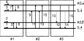
Figure 1: The 16 possible transitions between the single-particle energy levels in the UCS is divided in the GRPA into 3 uncoupled subsystems involving 8,4 and 4 transitions.

Transition $5$ corresponds to a pseudospin-wave mode first found in Ref. fertigdispersion, in which the pseudospins precess around their groundstate orientation. Solving Eq. (31), we find the general dispersion relation

$$\hslash^{2}\omega_{5}^{2}\left(q\right) = 4a\left(q\right)b\left(q\right)$$

$$+\left[\Delta_{b}+\sigma\left(X\left(0\right)-\widetilde{X}\left(q\right)-\frac{d}{\ell}\left(\frac{e^{2}}{\kappa\ell}\right)\right)\right]^{2},$$

where

$$a\left(q\right) = \frac{\Delta_{SAS}}{2}+\alpha\left[\widetilde{X}\left(0\right)-\widetilde{X}\left(q\right)\right],$$ (36)

$$b\left(q\right) = \frac{\Delta_{SAS}}{2}$$ (37)

$$+\alpha\left[\widetilde{X}\left(0\right)-X\left(q\right)+H\left(q\right)-\widetilde{H}\left(q\right)\right].$$

Using Eq. (34), it is easy to show that this mode is gapless if $\allowbreak\allowbreak\Delta_{SAS}=0$ even with finite bias. This is true as long as the interlayer coherence is non zero i.e. $\alpha\neq 0.$ At $q=0$, the pseudospins execute small oscillations in $x-y$ plane if the bias is zero while, at finite bias and $q=0$, they execute small oscillations in a plane where $\left\langle P_{z}\right\rangle=cst.$ In both cases, the energy cost is zero because the Hamiltonian of Eq. (II) is invariant with respect to a rotation in a plane of constant $\left\langle P_{z}\right\rangle$ if $\Delta_{SAS}=0.$ At finite tunneling, the pseudospin-wave mode is gapped with $\Delta_{SAS}^{\ast}$, the frequency at $q=0$, larger than $\Delta_{SAS}.$

The dispersion relations of the collective modes numbered $9,11,13,15$ are found by solving $\det B=0$ with the matrix $B$ given by

$$B=\left(\begin{array}[]{cccc}c_{1}-\nu_{1}X\left(q\right)&-\frac{\Delta_{SAS}}{2}&f-\alpha\widetilde{X}\left(q\right)&0\\ -\frac{\Delta_{SAS}}{2}&c_{1}-\nu_{1}\widetilde{X}\left(q\right)-\widetilde{\Delta}_{b}&0&f-\alpha X\left(q\right)\\ f-\alpha X\left(q\right)&0&c_{3}-\nu_{3}\widetilde{X}\left(q\right)+\widetilde{\Delta}_{b}&-\frac{\Delta_{SAS}}{2}\\ 0&f-\alpha\widetilde{X}\left(q\right)&-\frac{\Delta_{SAS}}{2}&c_{3}-\nu_{3}X\left(q\right)\end{array}\right).$$ (38)

In this equation, we have defined the constants

$$c_{1}=\Delta_{Z}+\nu_{1}X\left(0\right),$$ (39)

$$c_{3}=\Delta_{Z}+\nu_{3}X\left(0\right),$$ (40)

$$f=\frac{\Delta_{SAS}}{2}+\alpha\widetilde{X}\left(0\right),$$ (41)

$$\widetilde{\Delta}_{b}=\Delta_{b}+\left(\nu_{3}-\nu_{1}\right)\frac{d}{\ell}\left(\frac{e^{2}}{\kappa\ell}\right).$$ (42)

For zero bias (in which case $\alpha=1/2$), we can solve analytically to find the two dispersive modes

$$\hslash\omega_{11}\left(q\right) = \Delta_{Z}+\Delta_{SAS}$$

$$+\frac{1}{2}\left[X\left(0\right)+\widetilde{X}\left(0\right)-X\left(q\right)-\widetilde{X}\left(q\right)\right],$$

$$\hslash\omega_{13}\left(q\right) = \Delta_{Z}$$

$$+\frac{1}{2}\left[X\left(0\right)+\widetilde{X}\left(0\right)-X\left(q\right)-\widetilde{X}\left(q\right)\right].$$

The frequency $\omega_{13}\left(q\right)$ corresponds to the spin-wave (or Zeeman) mode in which the spins precess around their equilibrium orientations while mode $11$ involves a spin and pseudospin flip. At zero bias and $\Delta_{SAS}=0$, these two modes are degenerate at $q=0$ i.e. $\hslash\omega_{11}\left(0\right)=\hslash\omega_{13}\left(0\right)=\Delta_{Z}.$

Fig. 2 shows the evolution of the dispersion of the three modes $5,11,13$ with bias at $d/\ell=1,\Delta_{SAS}=0$, $\Delta_{Z}/\left(e^{2}/\kappa\ell\right)=0.2$ for (a) $\Delta_{b}/\left(e^{2}/\kappa\ell\right)=0,$ (b) $\Delta_{b}/\left(e^{2}/\kappa\ell\right)=0.1,$ and (c) $\Delta_{b}/\left(e^{2}/\kappa\ell\right)=0.4.$ For case (d), $\Delta_{b}/\left(e^{2}/\kappa\ell\right)=0.4$ and $\Delta_{SAS}/\left(e^{2}/\kappa\ell\right)=0.02$. Our numerical method also produces the frequency of the non-dispersive transitions $7,9,15$. We are not interested in these transitions as they have zero weigth in the response functions at zero temprature.

From Fig. 2, we see that there is one pseudospin mode and two spin-wave modes. We find that all three dispersions are affected by the bias. Figure 2(a) shows a roton minimum $\Delta_{b}/\left(e^{2}/\kappa\ell\right)=0.4$ increasing with interlayer separation indicating the instability of the UCS. Figures (b) and (c), show that an increase in the bias removes this roton mimimum.

The value $\Delta_{b}/\left(e^{2}/\kappa\ell\right)=0.2$ in Fig. 2(b) corresponds to the filling factors $\nu_{1}=0.38,\nu_{3}=0.62$ while the value $\Delta_{b}/\left(e^{2}/\kappa\ell\right)=0.4023$ in Fig. 2(c) corresponds to $\nu_{1}=0.00008,\nu_{3}=0.99992.$ Thus, the bias in Fig. 2(c) is just below the critical value above which the charge is completely transferred to the left well. It is easy to get analytical results for the asymptotic values ($q\rightarrow\infty$) of the modes in this case (i.e. the transport gaps). We need only solve Eq. (38) with $t=0,\nu_{R}=0$ and take $X\left(\mathbf{q}\right),\widetilde{X}\left(\mathbf{q}\right)\rightarrow 0$. We find a spin-wave (SW) and a spin-wave with pseudospin flid (SWPF) with dispersions $\hslash\omega_{SWPF}\left(q\rightarrow\infty\right)=$ $\Delta_{b}+\Delta_{Z}-\frac{d}{\ell}(e^{2}/\kappa\ell)+X\left(0\right)$ and $\hslash\omega_{SW}\left(q\rightarrow\infty\right)=\Delta_{Z}+X\left(0\right).$ In this limit, the $S$ and $AS$ symmetric states have evolved into the $L$ and $R$ states. The mode SW corresponds to a spin flip transition in the same well and its energy is $\hslash\omega_{SW}\left(q\rightarrow\infty\right)=\Delta_{Z}+X\left(0\right)$ since $X\left(0\right)$ is the energy required to remove an electron from the filled $L,\uparrow$ state. This mode is the spin-wave mode in a single quantum well system. Its dispersion relation at finite $q$ is given by

$$\hslash\omega_{SW}\left(\mathbf{q}\right)=\Delta_{Z}+X\left(0\right)-X\left(\mathbf{q}\right).$$ (45)

The mode SWPF involves a spin and a pseudospin flip and so a transition of an electron from the $L$ to the $R$ well. When the charge is completely transferred into the left well and we take into account the positive neutralizing backgrounds, there is an electric field oriented from the $R$ well to the $L$ well. There is thus a gain in energy $\frac{d}{\ell}(e^{2}/\kappa\ell)$ in transferring the charge from the $L$ to the $R$ well. The total energy to remove an electron from the filled $L,\uparrow$ state and create an infinitely separated electron-hole pair with spin and pseudospin flip is thus $\hslash\omega_{SWPF}\left(q\rightarrow\infty\right)=$ $\Delta_{b}+\Delta_{Z}-\frac{d}{\ell}(e^{2}/\kappa\ell)+X\left(0\right)$. With the parameters of Fig. 2, we find $\hslash\omega_{SW}\left(q\rightarrow\infty\right)=1.25(e^{2}/\kappa\ell)$ and $\hslash\omega_{SWPF}\left(q\rightarrow\infty\right)=0.85(e^{2}/\kappa\ell).$ The values are in good agreement with the numerical result plotted in Fig. 2(c). In Fig. 2(d), we have added a small tunnel coupling $\Delta_{SAS}/(e^{2}/\kappa\ell)=0.02$ that lifts the degeneracy of the two modes gapped at the Zeeman energy. At $q=0$, the ordering of these two modes is just the opposite than at $q\rightarrow\infty$. The Zeeman mode is gapped at $\hslash\omega_{SW}\left(0\right)=\Delta_{Z}$ while the pseudospin+spin flip mode is gapped at $\hslash\omega_{SWPF}\left(0\right)=\Delta_{Z}+\Delta_{SAS}.$

Figure 2: Dispersion relations of the collective excitations in the UCS at $\nu=1$ as computed in the GRPA. Parameters are $d/\ell=1,\Delta_{Z}/\left(e^{2}/\kappa\ell\right)=0.2$ and (a) $\Delta_{b}/\left(e^{2}/\kappa\ell\right)=0,\Delta_{SAS}=0$, (b) $\Delta_{b}/\left(e^{2}/\kappa\ell\right)=0.1,\Delta_{SAS}=0,$ (c) $\Delta_{b}/\left(e^{2}/\kappa\ell\right)=0.4023,\Delta_{SAS}=0,$ and (d) $\Delta_{b}/\left(e^{2}/\kappa\ell\right)=0.4,$ $\Delta_{SAS}/\left(e^{2}/\kappa\ell\right)=0.02.$ The straight lines give the frequency of the non-dispersive modes. The modes $5,11,13$ correspond to the dispersions $\omega_{5}\left(q\right),\omega_{11}\left(q\right),\omega_{13}\left(q\right)$ derived in the text. The abbreviations SW and SWPF refer to the spin-wave and spin-wave with pseudospin-flip modes (see text).

V Spin-Skyrmion crystals

If the electrical bias is sufficiently strong for all the charges to go into the left well, the system becomes effectively a single quantum well system (SQWS). The index $i$ then takes the values $i=3,4$ only. It is well known that, in this case, the ground state at $\nu=1$ is a spin ferromagnet. At small $\Delta_{Z}$, this state supports topological spin-texture excitations known as Skyrmionssondhi ; fertigskyrmion . Away from $\nu=1$, a finite density $n_{s}=\left|\nu-1\right|/2\pi\ell^{2}$ of Skyrmions is included in the the ground state and is expected to form a Skyrme crystalbreyprl . The Hartree-Fock ground state energy of the Skyrme crystal in a SQWS is, using Eq. (II),

$$\frac{E_{HF}}{N} = -\frac{\Delta_{Z}}{\nu}\left\langle S_{z}\left(\mathbf{0}\right)\right\rangle$$

$$+\frac{1}{4\nu}\sum_{\mathbf{G}}\Upsilon_{2}\left(\mathbf{G}\right)\left|\left\langle\rho\left(\mathbf{G}\right)\right\rangle\right|^{2}$$

$$-\frac{1}{\nu}\sum_{\mathbf{G}}X\left(\mathbf{G}\right)\left|\left\langle\mathbf{S}\left(\mathbf{G}\right)\right\rangle\right|^{2},$$

where we have defined

$$\Upsilon_{2}\left(\mathbf{G}\right)=2H\left(\mathbf{G}\right)-X\left(\mathbf{G}\right).$$ (47)

A Skyrme crystal has a noncollinear magnetic order. A single Skyrmion spin texture of such a crystal has its spins aligned with the Zeeman field at infinity, reversed at the center of the Skyrmion, and has nonzero $XY$ spin components at intermediate distances which have a vortex-like configuration (see Fig. 3(a)). The classical (or quantum mean field) energy of a Skyrmion is independent of the angle $\varphi$ which defines the global orientation of the $XY\$spin component. This independence gives an extra $U\left(1\right)$ degree of freedom for a single Skyrmion. In a crystal of Skyrmions, this $U\left(1\right)$ symmetry is spontaneously broken and the crystal has an extra Goldstone mode. We refer to this mode as the $XY\$mode because it corresponds to an oscillation of the perpendicular component of the spins in the $x-y$ plane with $\left\langle S_{z}\right\rangle$ fixed. From Eq. (V), we see that such a motion costs no energy provided the density $\left\langle\rho\left(\mathbf{G}\right)\right\rangle$ is not changed. That this is the case can be seen from the fact that the relation between the topological charge and the spin textureleekane is given at $\nu=1$ by (the sum over indices is implicit)

$$\delta\left\langle n\left(\mathbf{r}\right)\right\rangle=-\frac{1}{8\pi}\varepsilon_{abc}s_{a}\left(\mathbf{r}\right)\varepsilon_{ij}\partial_{i}s_{b}\left(\mathbf{r}\right)\partial_{j}s_{c}\left(\mathbf{r}\right),$$ (48)

where $\varepsilon_{ij}$ and $\varepsilon_{abc}$ are antisymmetric tensors, with $i,j=x,y$ and $a,b,c=x,y,z$, and $\mathbf{s}\left(\mathbf{r}\right)$ is a classical field with unit modulus representing the spins. If we write a general spin texture as

$$s_{x}\left(\mathbf{r}\right) = \sin\left[\theta\left(\mathbf{r}\right)\right]\cos\left[\varphi\left(\mathbf{r}\right)\right],$$ (49)

$$s_{y}\left(\mathbf{r}\right) = \sin\left[\theta\left(\mathbf{r}\right)\right]\sin\left[\varphi\left(\mathbf{r}\right)\right],$$ (50)

$$s_{z}\left(\mathbf{r}\right) = \cos\left[\theta\left(\mathbf{r}\right)\right],$$ (51)

then the induced density takes the simple form

$$\delta n\left(\mathbf{r}\right)=\frac{1}{4\pi}\sin\left[\theta\left(\mathbf{r}\right)\right]\left[\nabla\theta\left(\mathbf{r}\right)\times\nabla\varphi\left(\mathbf{r}\right)\right]\cdot\widehat{\mathbf{z}}.$$ (52)

Clearly, the induced charge density in the $XY$ mode is zero because $\nabla\varphi\left(\mathbf{r}\right)$ is unchanged if we rotate all the spins by the same angle (i.e. $\varphi\left(\mathbf{r}\right)\rightarrow\varphi\left(\mathbf{r}\right)+cst$).

The phase diagram of the 2DEG around $\nu=1$ has been studied in the HFA in Refs. breyprl, ; cotegirvinprl, ; breymerons, . In a large portion of the $\nu-\Delta_{Z}$ phase space, the Hartree-Fock ground state is a square lattice with two Skyrmions of opposite global phase $\varphi$ per unit cell as shown in Fig. 3(a). This configuration is called SLA (Square Lattice Antiferromagnet) to account for the phases $\varphi=0$ and $\varphi=\pi$ of the two Skyrmions in the unit cell. As the Zeeman energy is increased, our Hartree-Fock approximation (HFA)cotegroup1 shows that there is a transition to a triangular lattice of Skyrmions with a phase difference of $\varphi=2\pi/3$ between the three Skyrmions in a unit cell and then to a triangular Wigner crystal of spin down electrons with no spin texture.

Note that the size of the individual Skyrmions in the Skyrme crystal is determined in part by the Zeeman energy $\Delta_{Z}$. For large $\Delta_{Z},$ the tipping of spins into the minority direction that occurs in the spin texture of a skyrmion becomes energetically unfavorable, and Skyrmions become relatively small. For decreasing $\Delta_{Z}$, the Skyrmions become larger until their size is limited by inter-Skyrmion interactions. For small enough Zeeman coupling the system undergoes a transition into a meron crystalbreymerons with four merons per unit cell as shown in Fig. 3(b).

A meron is most easily visualized by rotating the spin axes around the $y$ axis so that the $z$ axis becomes the $x$ axis and the $x$ axis becomes the $-z$ axis. In this basis a meron has its spin down or up at the origin and lies in the $XY$ plane at infinity with a vortex-like structure. The vorticity can be positive or negative so that, combined with the up or down spins at the origin, there are four possible types of merons. In the rotated basis, one can recognize the Skyrmion as a bound meron-antimeron pair (i.e., a bimeron). Hartree-Fock calculationscotegroup1 shows that the meron crystal is stable only at filling factors $\nu>1.38.$ For smaller filling factors, we find, as suggested in Ref. nazarov, , that Skyrmions always appear in pairs to form a triangular Wigner lattice. There is an attractive interaction between Skyrmions with opposite phases which prevails over the Coulomb repulsion at large separations between the Skyrmions. Thus, as the Zeeman energy is reduced and for $\nu_{c}<\nu<1.38$ where $\nu_{c}\approx 1.06$, there is a transition from the Skyrme crystal to a crystal of biskyrmions. In Ref. nazarov, , the minimal energy is found for zero separation between the pairs of Skyrmions in a biskyrmion leading to a Skyrmion with topological charge $Q=2.$ Within the HFA, there is a finite separation between the two Skyrmions in each pair.

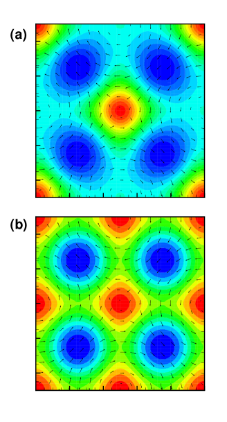
Figure 3: (Color online) Spin texture in the $x-y$ plane (vectors) and density in a unit cell of a Skyrme lattice in (a) the SLA and (b) the meron configurations at $\nu=1.30$ with $\Delta_{Z}/\left(e^{2}/\kappa\ell\right)=0.01$ and $\Delta_{Z}/\left(e^{2}/\kappa\ell\right)=0$ respectively. In (a), $S_{z}=-\frac{1}{2}$ at the position of the Skyrmions and each Skyrmion carries charge $q=-e.$ In (b), $S_{z}=-\frac{1}{2}$ at the positions of the four merons at the corner of the unit cell and at the position of the meron at the center while $S_{z}=+\frac{1}{2}$ at the positions of the other merons. Each merons carries a charge $q=-\frac{e}{2}.$ Contours with dark (red) regions indicate a high density.

The low-energy collective modes of the Skyrmecotegirvinprl and meron crystals computed in the GRPA are shown in Fig. 4. The dispersions are shown for wavevector $\mathbf{k}$ along the path $\Gamma-M-X-\Gamma$ around the irreducible Brillouin zone as shown in the inset of Fig. 4(b). The low-energy part of the spectrum consists of two gapless (Goldstone) and two gapped modes. One of the Goldstone mode is the phonon mode which is due to the spontaneously broken translational symmetry in the crystal. Its dispersion is $\omega\sim k^{3/2}$ which is similar to that of a Wigner crystal in a magnetic field. The second Goldstone mode is the $XY$ mode introduced above. This gapless mode is believed to be responsiblecotegirvinprl ; green for the small spin-lattice relaxation time $T_{1}$ measured in NMR experimentsbarret on both sides of $\nu=1$.

Of the two gapped branches, one has a gap that varies with $\Delta_{Z}$ and $\nu$ and the other is gapped at exactly the Zeeman energy for all $\nu$ as required by Larmor’s theorem. This last mode is obviously a spin wave mode where the spins precess around their local orientation. We refer to this mode as the Zeeman mode. In the first mode, the motion of the two Skyrmions with opposite global phases $\varphi$ in a unit cell (as seen in our animationsanimation ) are out of phase. We identify this mode as an optical phonon mode.

At $\nu=1.2,$ the two gapped branches are degenerate at $\mathbf{k}=0$. For $\nu>1.2,$ the spin-wave branch is connected to the phonon branch at point $M$ as in Fig. 4(a) while for $\nu\leq 1.2,$ it is connected to the $XY$ spin mode. The gap in both branches goes to zero as $\Delta_{Z}\rightarrow 0$ so that, in the meron crystal, all four branches are gapless as seen in Fig. 4(b).

We can understand the origin of the three gapless modes (in addition to the phonon mode) in a spin-meron crystal when $\Delta_{Z}=0$ by the fact that the energy of such a spin texture is invariant with respect to a rotation of the spins around three orthogonal directions. Because these three symmetries are spontaneously broken in the meron crystal, we get three Goldstone modes corresponding, in our case, to oscillations in the $x-y,y-z$ and $x-z$ planes. This interpretation is confirmed by our animations of these modesanimation . There is no motion of the charge in any of these three modes, the optical phonon mode present when $\Delta_{Z}\neq 0$, i.e. in the Skyrme crystal, is presumably to be found amongst the higher-energy modes not considered in our study. As $\Delta_{Z}\rightarrow 0$, the out of phase motion of the Skyrmions in the optical phonon mode gradually stops until it disappears completely in the meron crystal.

In Fig. 4 and other similar figures, we plot the poles with the two (six for the $CP^{3}$ case below) biggest weights in the response functions indicated in the legend. The function $\chi_{xx}$ stands for $\chi_{S_{x},S_{x}},$ $\chi_{yy}$ stands for $\chi_{S_{y},S_{y}}$ etc. For very small wavevector $\mathbf{k}$, this gives an indication of the nature of the mode. The phonon mode, for example, is strongest in the density response $\chi_{n,n}$ while the $XY$ mode is strongest in $\chi_{zz}$.

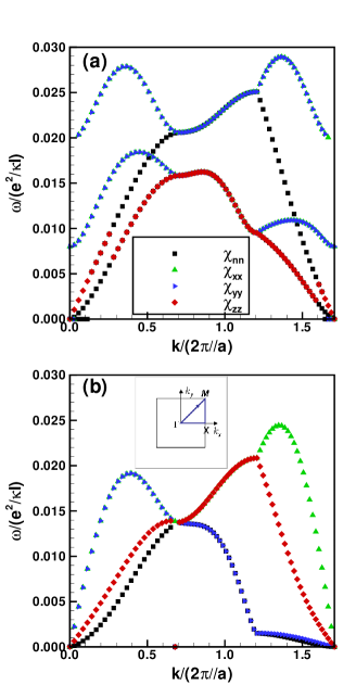
Figure 4: (Color online) Dispersion relation of the collective modes of the Skyrme crystal for a (a) SLA configuration with $\nu=1.30$ and $\Delta_{Z}/\left(e^{2}/\kappa\ell\right)=0.008$ and (b) a meron configuration similar to that of Fig. 3(b) but with $\nu=1.38$ and $\Delta_{Z}/\left(e^{2}/\kappa\ell\right)=0.$ The dispersion is computed along the path $\Gamma-M-X-\Gamma$ in the Brillouin zone as shown by the inset in Fig. 4(b). The symbols indicate from what response function each frequency comes. The softening of the modes seen in (b) is due to the meron crystal becoming unstable at $\nu=1.36$ with respect to a biskyrmion crystal.

VI Pseudospin-Skyrmion crystals

If the spin degree of freedom is neglected, then the 2DEG in a DQWS can be described by its pseudospin and charge orders only. In the absence of bias, the ground state at $\nu=1$ is a pseudospin ferromagnetmacdobible . For nonzero interlayer separation $d,$ all pseudospins are forced to lie in the $XY$ plane in order to minimise the capacitive energy (the term $J_{z,2}\left(0\right)\left|\left\langle P_{z}\left(0\right)\right\rangle\right|^{2}$ in Eq. (VI) below). The charged excitations of this system are pseudospin-Skyrmions or bimeronsmacdobible . A finite density of bimerons is included in the ground state when $\nu\neq 1$. Once again, these topological excitations should form a crystal at zero temperature. The Hartree-Fock ground-state energy is written, in the pseudospin language, as

$$\frac{E_{HF}}{N} = -\frac{\Delta_{SAS}}{\nu}\left\langle P_{x}\left(\mathbf{0}\right)\right\rangle$$

$$+\frac{1}{4\nu}\sum_{\mathbf{G}}\Upsilon_{2}\left(\mathbf{G}\right)\left|\left\langle\rho\left(\mathbf{G}\right)\right\rangle\right|^{2}$$

$$+\frac{1}{\nu}\sum_{\mathbf{G}}J_{z,2}\left(\mathbf{G}\right)\left|\left\langle P_{z}\left(\mathbf{G}\right)\right\rangle\right|^{2}$$

$$-\frac{1}{\nu}\sum_{\mathbf{G}}\widetilde{X}\left(\mathbf{G}\right)\left|\left\langle\mathbf{P}_{\bot}\left(\mathbf{G}\right)\right\rangle\right|^{2},$$

where

$$J_{z,2}\left(\mathbf{G}\right)=H\left(\mathbf{G}\right)-\widetilde{H}\left(\mathbf{G}\right)-X\left(\mathbf{G}\right),$$ (54)

and

$$\mathbf{P}_{\bot}\left(\mathbf{G}\right)=P_{x}\left(\mathbf{G}\right)\widehat{\mathbf{x}}+P_{y}\left(\mathbf{G}\right)\widehat{\mathbf{y}}.$$ (55)

The interlayer coherence (i.e. $\left\langle\mathbf{P}_{\bot}\left(\mathbf{q}\right)\right\rangle\neq 0$) is lost at some critical interlayer separation which is of the order of $d/\ell\approx 1.2$ at zero bias and tunneling. In the coherent regime, the phase diagram in the $d/\ell-\Delta_{SAS}-\nu$ space is very rich and has been only partially studiedbreycristalbimerons ,cotegroup1 . In analogy with the phase diagram of the Skyrme crystal in a SQWS, we find, in some regions of the parameter space where $\Delta_{SAS}\neq 0,$ a solution consisting of a square lattice with two bimerons of opposite global phases $\varphi$ and meron-antimeron orientation reversed per unit cell. We call this phase an SLA bimeron crystal. An example of such crystal is given in Fig. 5. Near zero tunneling, we get a crystal of merons with four merons per unit cell in exactly the same $SLA\$configuration as that of the spin-meron crystal shown in Fig. 3(b).

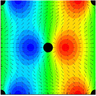
Figure 5: (Color online) Pseudospin texture in the $x-y$ plane (vectors) and value of $S_{z}$ (contours) in a unit cell of a bimeron crystal in a SLA configuration with $\nu=1.20$ and $\Delta_{SAS}/\left(e^{2}/\kappa\ell\right)=0.02.$ The full black circles indicate the position of the maximum in the bimeron density. Dark (red) contours correspond to $S_{z}=+\frac{1}{2}$ while gray (blue) contours are for $S_{z}=-\frac{1}{2}.$ Note that the pseudospin texture for the bimeron at the center has a global phase rotation of with respect to the pseudospin texture of the bimerons at the four corners of the unit cell.

The collective mode spectrum of a bimeron crystal is shown in Fig. 6 where again we have plotted the four lowest branches only. There is one gapless and three gapped modes. The gapless mode is the phonon mode, which appears as a pole of $\chi_{nn}$ and has a $\omega\sim k^{3/2}$ dispersion as in the Skyrme crystal. The next lowest mode has a very small gap that closes as the interlayer separation $d\rightarrow 0$ even when tunneling is finite. In this gapless limit it has a linear dispersion. This behavior is easily understood: when $d=0$ and $\Delta_{SAS}=0$, a bimeron crystal can be mapped onto a Skyrme crystal with zero Zeeman coupling. (A bimeron is obtained by rotating the spin texture of a Skyrmion by $90$ degrees around the spin $x$ or $y$ axis.) If one rotates around the $y$ axis, the resulting bimeron has pseudospins lying along the $x$ direction at infinity, with the two merons aligned along the $x$ axis. The tunneling term $\Delta_{SAS}S_{x}$ for the bimeron crystal then plays the role of the Zeeman term $\Delta_{Z}S_{z}$ in the Skyrme crystal. It follows that, for $d=0$, the collective modes of the bimeron crystal are identical to that of Skyrme crystal with $\Delta_{Z}=\Delta_{SAS}.$ However, the specific modes appear in different response functions. When $d=0$ but tunneling is finite, Eq. (VI) becomes

$$\frac{E_{HF}}{N} = -\frac{\Delta_{SAS}}{\nu}\left\langle P_{x}\left(\mathbf{0}\right)\right\rangle$$

$$+\frac{1}{4\nu}\sum_{\mathbf{G}}\Upsilon_{2}\left(\mathbf{G}\right)\left|\left\langle\rho\left(\mathbf{G}\right)\right\rangle\right|^{2}$$

$$-\frac{1}{\nu}\sum_{\mathbf{G}}X\left(\mathbf{G}\right)\left|\left\langle\mathbf{P}\left(\mathbf{G}\right)\right\rangle\right|^{2},$$

From Eq. (VI), we see that the pseudospins can rotate freely in the $y-z$ plane but not in the $x-y$ plane if $\Delta_{SAS}\neq 0$. The $XY$ Goldstone mode of the Skyrme crystal becomes a $YZ$ Goldstone mode in the bimeron crystal at $d=0$. At finite interlayer separation $H\left(\mathbf{G}\right)\neq\widetilde{H}\left(\mathbf{G}\right)$ and $X\left(\mathbf{G}\right)\neq\widetilde{X}\left(\mathbf{G}\right)$ and a rotation in the $y-z$ plane can no longer be performed without energy cost. The $YZ$ mode is thus gapped at finite interlayer separation.

We can explain the smallnest of this gap in the following way. A global rotation of the pseudospins in the $y-z$ plane leads to a solid rotation of the bimerons (i.e. a rotation of the pairs of merons around the filled black circles in Fig. 5). At $d=0$, the bimeron density is circularly symmetricbreycristalbimerons and so does not change under a rotation of the bimeron. At finite $d$, however, the bimeron density is no longer circularly symmetric. A rotation of an isolated bimeron would not change its energy but, in a crystal, these charged objects interact with one another via the Coulomb interaction, so there is an energy cost for such rotations. The energy cost, however, is small because it comes from high order multipole interactions. (The rotation of the bimerons can be clearly seen in the animationsanimation .)

At $d\neq 0$ but $\Delta_{SAS}=0$ (in which case we get a meron crystal), a rotation of the pseudospins in the $x-y$ plane without an energy cost is possible. This in this limit a meron crystal has a gapless $XY\$mode (see Fig. 7) just as a Skyrme crystal.

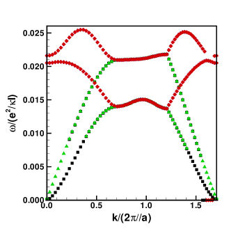
Figure 6: (Color online) Collective mode spectrum of a bimeron crystal in the SLA configuration of Fig. 5 with $\nu=1.2,\Delta_{SAS}/\left(e^{2}/\kappa\ell\right)=0.02$ and $d/\ell=0.1.$ The path in the Brillouin zone is as indicated in the inset of Fig. 4(b) and the symbols are as indicated in the legend of that same figure.

The interlayer-coherent homogeneous phase at $\nu=1$ can sustainfertigdispersion a pseudospin-wave mode in which the pseudospins execute small precession around their local equilibrium direction (the $x$ axis for $\Delta_{SAS}\neq 0$). The pseudospin-wave mode is equivalent to the spin-wave (or Zeeman) mode in the Skyrme crystal. We discussed this mode before in Sec. IV. Its dispersion is given by Eq. (IV). For $\Delta_{SAS}=0$, the dispersion $\omega_{5}\left(q\right)$ is linear in $q$ for small wavevector. This mode has been detected experimentallyspielmanpseudospinmode . For $\Delta_{SAS}\neq 0$ and $d=0$, the pseudospin-wave mode is gapped at $\omega_{PSW}\left(0\right)=\Delta_{SAS}$ as can be seen from Eq. (IV). At finite $d$, that gap is increased. In Fig. 6, $d$ is small and we see two modes gapped at a value near $\Delta_{SAS}$. If we replace $\left\langle\rho_{1,3}\left(0\right)\right\rangle,\nu_{R}$ and $\nu_{L}$ by their values in the crystal phases in Eq. (IV), we get a very good estimate of the pseudospin-wave gap $\omega_{5}\left(0\right)$ in the bimeron crystal. In the example of Fig. 6, $d/\ell=0.1,$ $\left\langle\rho_{1,3}\left(0\right)\right\rangle=0.106$ and $\nu_{R}=\nu_{L}=0.6$ so that we find $\omega_{5}\left(0\right)=0.021\left(e^{2}/\hslash\kappa\ell\right)$ which is in good agreement with the computed gap. We find excellent agreement for other values of $d/\ell$ as well. This permits us to identify the higher-energy dispersion branch as the pseudospin-wave mode. Our animationsanimation show that the other high-energy branch is an optical phonon mode in which the two bimerons in the unit cell have opposite motions.

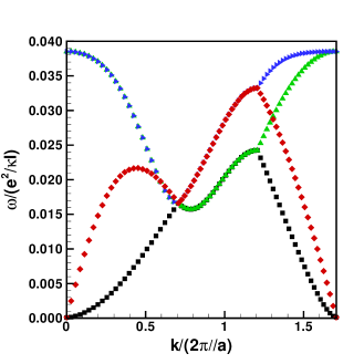
Figure 7: (Color online) Collective mode spectrum of a pseudospin meron crystal in a SLA configuration similar to that of Fig. 3(b) with $\nu=1.2,\Delta_{SAS}/\left(e^{2}/\kappa\ell\right)=0$ and $d/\ell=0.8$. The path in the Brillouin zone is as indicated in the inset of Fig. 4(b) and the symbols are as indicated in the legend of that figure.

Figure 7 shows the collective mode spectrum of a pseudospin meron crystal. The two gapless modes are the phonon and the $XY$ mode as discussed above and the other two branches are the optical phonon and pseudospin-wave modes. These two branches are degenerate along $\Gamma M$ at all $d/\ell$ for the SLA configuration. Eq. (IV) fails in this case since $\left\langle\rho_{1,3}\left(0\right)\right\rangle=0$ for a meron crystal (but $\left\langle\rho_{1,3}\left(\mathbf{G}\neq 0\right)\right\rangle\neq 0$) and we get $\omega_{5}\left(0\right)=0$ for all interlayer separations. That this equation works for the bimeron crystal but fails for the meron crystal can be understood by the fact that the bimeron crystal has regions of coherent liquid between the bimerons whereas the meron crystal has no such regions.

VII CP³ Skyrmion crystals

Now that we understand the limiting cases of pure spin and pure pseudospin crystals, we are ready to look at the collective excitations of the $CP^{3}$ Skyrmion crystal with has entangled spin and pseudospin textures. We study the excitation spectrum as a function of interlayer separation, tunneling, and bias as was done for the ground state in Paper Icotecp3 . We refer the reader to this paper for the definition of the various groundstates that we will use in the present section. We remark that all our data for the $CP^{3}$ Skyrmion crystal in this section are for filling factor $\nu=0.8$ where we get a good convergence of the order parameters for the $CP^{3}$ phases. For $\nu>1.0,$ a similar phase is difficult to find numerically (see Paper Icotecp3 ). For the spin-Skyrmion and pseudospin-Skyrmion crystals, our results above were for $\nu>1.0.$ In these two cases, however, the phase diagram below $\nu=1$, can be related to that above $\nu=1$ by particle-hole symmetry. In the $CP^{3}$ Skyrmion case, there is no such particle-hole symmetry.

The groundstate energy of Eq. (II) can be written in the spin-pseudospin langage as

$$\frac{E_{HF}}{N}=\frac{\Delta_{b}}{\nu}\left\langle P_{z}\left(\mathbf{0}\right)\right\rangle-\frac{\Delta_{Z}}{\nu}\left\langle S_{z}\left(\mathbf{0}\right)\right\rangle-\frac{\Delta_{SAS}}{\nu}\left\langle P_{x}\left(\mathbf{0}\right)\right\rangle$$

$$+\frac{1}{4\nu}\sum_{\mathbf{G}}\Upsilon_{1}\left(\mathbf{G}\right)\left|\left\langle\rho\left(\mathbf{G}\right)\right\rangle\right|^{2}+\frac{1}{\nu}\sum_{\mathbf{G}}J_{z,1}\left(\mathbf{G}\right)\left|\left\langle P_{z}\left(\mathbf{G}\right)\right\rangle\right|^{2}$$

$$-\frac{1}{\nu}\sum_{\mathbf{G}}\sum_{a=R,L}X\left(\mathbf{G}\right)\left|\left\langle\mathbf{S}_{a}\left(\mathbf{G}\right)\right\rangle\right|^{2}$$ (57)

$$-\frac{1}{\nu}\sum_{\mathbf{G}}\sum_{\alpha=+,-}\widetilde{X}\left(\mathbf{G}\right)\left[\left|\left\langle P_{x,\alpha}\left(\mathbf{G}\right)\right\rangle\right|^{2}+\left|\left\langle P_{y,\alpha}\left(\mathbf{G}\right)\right\rangle\right|^{2}\right]$$

$$-\frac{1}{\nu}\sum_{\mathbf{G}}\widetilde{X}\left(\mathbf{G}\right)\left[\left|\left\langle\rho_{1,4}\left(\mathbf{G}\right)\right\rangle\right|^{2}+\left|\left\langle\rho_{2,3}\left(\mathbf{G}\right)\right\rangle\right|^{2}\right],$$

where we have defined the interactions

$$\Upsilon_{1}\left(\mathbf{G}\right) = H\left(\mathbf{G}\right)+\widetilde{H}\left(\mathbf{G}\right)-\frac{1}{2}X\left(\mathbf{G}\right),$$ (58)

$$J_{z,1}\left(\mathbf{G}\right) = H\left(\mathbf{G}\right)-\widetilde{H}\left(\mathbf{G}\right)-\frac{1}{2}X\left(\mathbf{G}\right),$$ (59)

and the fields (see Eq. (12))

$$P_{x,+}\left(\mathbf{G}\right)=\frac{1}{2}\left[\left\langle\rho_{1,3}\right\rangle+\left\langle\rho_{3,1}\right\rangle\right],$$ (60)

$$P_{x,-}\left(\mathbf{G}\right)=\frac{1}{2}\left[\left\langle\rho_{2,4}\right\rangle+\left\langle\rho_{4,2}\right\rangle\right],$$ (61)

$$P_{y,+}\left(\mathbf{G}\right)=\frac{1}{2i}\left[\left\langle\rho_{1,3}\right\rangle-\left\langle\rho_{3,1}\right\rangle\right],$$ (62)

$$P_{y,-}\left(\mathbf{G}\right)=\frac{1}{2i}\left[\left\langle\rho_{2,4}\right\rangle-\left\langle\rho_{4,2}\right\rangle\right].$$ (63)

In Eq. (57), $S_{i}=\sum_{a=R,L}S_{i,a}$ and $P_{i}=\sum_{\alpha=+,-}P_{i,\alpha}$ where $i=x,y,z.$ The total density is defined by

$$\left\langle\rho\left(\mathbf{G}\right)\right\rangle=\left\langle\rho_{11}\left(\mathbf{G}\right)\right\rangle+\left\langle\rho_{22}\left(\mathbf{G}\right)\right\rangle+\left\langle\rho_{33}\left(\mathbf{G}\right)\right\rangle+\left\langle\rho_{44}\left(\mathbf{G}\right)\right\rangle.$$ (64)

We will also make used of the fields

$$R_{xx}(\mathbf{q}) = \frac{1}{2}\left[\rho_{1,4}(\mathbf{q})+\rho_{4,1}(\mathbf{q})+\rho_{2,3}(\mathbf{q})+\rho_{3,2}(\mathbf{q})\right],$$ (65)

$$R_{zz}(\mathbf{q}) = \frac{1}{2}\left[\rho_{1,1}(\mathbf{q})-\rho_{2,2}(\mathbf{q})-\rho_{3,3}(\mathbf{q})+\rho_{4,4}(\mathbf{q})\right].$$ (66)

VII.1 Variation with interlayer separation

At small value $\Delta_{SAS}/\left(e^{2}/\kappa\ell\right)=0.0002<<\Delta_{Z}/\left(e^{2}/\kappa\ell\right)$ of the tunneling parameter, the ground state of the 2DEG at small interlayer separation $d/\ell$ is a spin-polarized meron crystal with an SLA configurationcotecp3 . The corresponding excitation spectrum is shown in Fig. 8. For all the following dispersion plots, we represent the poles of $\chi_{nn}$ by the full (black) circles, those of the pseudospin response functions $\chi_{\mathbf{PP}}$ by the empty (blue) squares, those of the spin response functions $\chi_{\mathbf{SS}}$ by the right (red) triangles and by the left (green) triangles the poles of the two response functions $\chi_{R_{xx},R_{xx}}$ and $\chi_{R_{zz},R_{zz}}$. The operator $R_{xx}$ (see Eq. (65)) involves a change in both the spin and pseudospin indices unlike the operators $\mathbf{S},\mathbf{P}$ or $n$. There are clearly two basic mode structures in Fig. 8. One, noted “(1)” is the pseudospin meron crystal response already studied in Fig. 7 and it comprises four branches. The second structure, noted “(2)”, has two twice-degenerate branches for a total of eight branches for the whole $CP^{3}$ crystal (considering the low-energy modes only since other higher-energy modes are also present in the GRPA). One branch in (2) is the Zeeman mode (gapped at $\Delta_{Z}/\left(e^{2}/\kappa\ell\right)=0.004$) while the other, which is also gapped, seems to appear predominantly in $\chi_{R_{xx}R_{xx}}$ and $\chi_{R_{zz}R_{zz}}$.

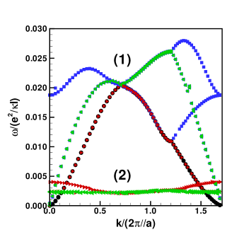
Figure 8: (Color online) Collective mode spectrum of a spin-polarized meron crystal with parameters: $\nu=0.8,\Delta_{Z}/\left(e^{2}/\kappa\ell\right)=0.004,\Delta_{SAS}/\left(e^{2}/\kappa\ell\right)=0.0002,\Delta_{b}/\left(e^{2}/\kappa\ell\right)=0,$ and $d/\ell=0.3.$

Figure 9 shows what happens to this collective mode spectrum when we increase the interlayer separation and keep both $\Delta_{SAS}$ and $\Delta_{Z}$ fixed. In this case (see Fig. 3 of Paper Icotecp3 ), the ground state becomes a $CP^{3}$ crystal at a critical layer separation $d_{c}$ that increases with $\Delta_{Z}$. For $\Delta_{Z}/\left(e^{2}/\kappa\ell\right)=0.004$, we find $d_{c}/\ell\approx 0.6$. In Fig. 9, $d/\ell=1.0$ and we see that the degeneracy of the modes in the structure (2) of Fig. 6 has been lifted and that two seemingly gapless modes have emerged from the lowest branch. In fact, the gap in the lowest branch in structure (2) vanishes continuously as the transition is approached. We believe that this should be observable experimentally. In the following analysis, it will become clear that of these two modes, one only one is truly gapless. We have identified the phonon, pseudospin-wave, pseudospin-$YZ$, and Zeeman modes in Fig. 9. We find that at $d/\ell=1.1$, the modes of structure (2) become soft at point $M$ in the Brillouin zone indicating an instability of the $CP^{3}$ crystal analogous to that of the uniform ($\nu=1$) system at similar separations fertigdispersion .

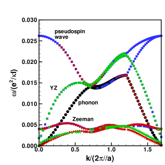
Figure 9: (Color online) Collective mode spectrum of a crystal of $CP^{3}$ Skyrmions along path -M-X- in the Brillouin zone. The parameters are: $\nu=0.8,\Delta_{Z}/\left(e^{2}/\kappa\ell\right)=0.004,\Delta_{SAS}/\left(e^{2}/\kappa\ell\right)=0.0002,\Delta_{b}/\left(e^{2}/\kappa\ell\right)=0,$ and $d/\ell=1.0.$

VII.2 Variation with tunnel coupling

To check if the two modes in Fig. 9 are really gapless, we plot in Fig. 10 the collective mode spectrum of the $CP^{3}$ crystal at a higher value of tunneling. In Paper Icotecp3 it was shown that when tunneling is increased, there is a transition from the $CP^{3}$ crystal state to a symmetric Skyrmion (SS) state. The SS is basically a pseudospin polarized spin-Skyrmion state in which the $S,\uparrow$ and $S,\downarrow$ only are occupied. There is thus a spin texture on top of a state where all pseudospins point along the $x$ axis. For Fig. 10, we choose $d/\ell=1.0,\Delta_{Z}/\left(e^{2}/\kappa\ell\right)=0.008$ and $\Delta_{SAS}/\left(e^{2}/\kappa\ell\right)=0.0044$. From Fig. 5(c) of Paper I, the ground state of the 2DEG is a SS state in this case. The $CP^{3}$ Skyrmion state is still stable even if is not the ground state and, as we see from Fig. 10, there is a very small gap with energy smaller than $0.001\left(e^{2}/\kappa\ell\right)$ in one of the two modes of structure 2. As we will show below, the application of an electrical bias does not open new gaps in the system so that we conclude that with finite bias, Zeeman, and tunneling energies, our $CP^{3}$ crystal has two Goldstone modes: the phonon mode and a phase mode whose origin we will discuss below.

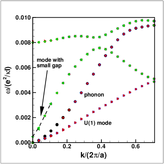
Figure 10: (Color online) Collective mode spectrum of a crystal of $CP^{3}$ Skyrmions with strong tunneling. The parameters are: $\nu=0.8,\Delta_{Z}/\left(e^{2}/\kappa\ell\right)=0.008,\Delta_{SAS}/\left(e^{2}/\kappa\ell\right)=0.0044,\Delta_{b}/\left(e^{2}/\kappa\ell\right)=0,$ and $d/\ell=1.0.$

The collective mode spectrum of a SS state at $d/\ell=1.0,\Delta_{Z}/\left(e^{2}/\kappa\ell\right)=0.008$ and $\Delta_{SAS}/\left(e^{2}/\kappa\ell\right)=0.0044$ is shown in Fig. 11. For $\Delta_{Z}/\left(e^{2}/\kappa\ell\right)=0.008$, the transition to the SS state occurs at $\Delta_{SAS}^{(c)}/\left(e^{2}/\kappa\ell\right)\approx 0.004$ which is roughly $\Delta_{SAS}^{(c)}\approx 0.5\Delta_{Z}$. The phonon and spin mode dispersions in Fig. 11 modes are typical of that of a Skyrme crystal (see Fig. 4(a)). There are only two gapless modes: the phonon and spin $XY$ phase mode.

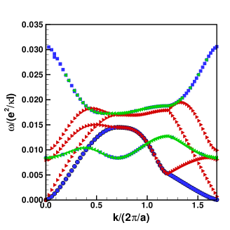
Figure 11: (Color online) Collective mode spectrum of a crystal of symmetric Skyrmions. The parameters are: $\nu=0.8,\Delta_{Z}/\left(e^{2}/\kappa\ell\right)=0.008,\Delta_{Z}/\left(e^{2}/\kappa\ell\right)=0.006,\Delta_{b}/\left(e^{2}/\kappa\ell\right)=0$, and $d/\ell=1.0.$

VII.3 Variation with electrical bias

We now turn on the bias between the two wells so that all the charge is gradually transferred to the left well. If we start with a $CP^{3}$ crystal at zero bias, our Hartree-Fock analysis (see Fig. 9 of Paper Icotecp3 ) shows that the spin and pseudospin textures are maintained until the charge has completely gone into one well and we get a spin-Skyrmion crystal. From the collective mode spectrum in Fig. 12, we see that the two Goldstone modes are preserved at finite bias if we consider that one of the low-energy mode has an extremely small gap (whose origin we explain in the next section). The qualitative features of the spectrum are unchanged from that of Fig. 9. The $CP^{3}$ crystal is stable up to the largest bias for which there is a charge in the right well. When the charge is completely transferred to the left well, the spectrum is that of the Skyrme crystal shown in Fig. 4(a).

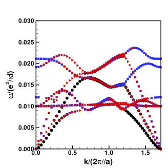
Figure 12: (Color online) Collective mode spectrum of a crystal of $CP^{3}$ Skyrmions with a finite bias. The parameters are: $\nu=0.8,\Delta_{Z}/\left(e^{2}/\kappa\ell\right)=0.01,\Delta_{SAS}/\left(e^{2}/\kappa\ell\right)=0.0002,\Delta_{b}/\left(e^{2}/\kappa\ell\right)=0.20$ and $d/\ell=1.0.$

VII.4 Physical origin of the Goldstone modes

Following Gosh and Rajaramanrajaramancp3 , we pametrize a general $CP^{3}$ spinor by six angles that can be roughly interpreted as the polar and azimuthal angles of the spins in the right and left wells: $\theta_{R},\theta_{L}$ and $\varphi_{R},\varphi_{L},$ and the polar and azimuthal angles of the total pseudospin, $\alpha$ and $\beta$. Writing

$$a\left(X\right)=\left(\begin{array}[]{c}\cos\frac{\alpha}{2}\cos\frac{\theta_{R}}{2}\\ \cos\frac{\alpha}{2}\sin\frac{\theta_{R}}{2}e^{i\varphi_{R}}\\ \sin\frac{\alpha}{2}\cos\frac{\theta_{L}}{2}e^{i\beta}\\ \sin\frac{\alpha}{2}\sin\frac{\theta_{L}}{2}e^{i\left(\beta+\varphi_{L}\right)}\end{array}\right),$$ (67)

a possible spin-pseudospin texture state can be written as

$$\left|\Psi\right\rangle=\prod\limits_{X}\left[\sum_{\sigma}a_{\sigma}\left(X\right)c_{\sigma,X}^{{\dagger}}\right]\left|0\right\rangle,$$ (68)

where $\left|0\right\rangle$ is the vacuum state. We replacerajaramancp3 $X$ by $\mathbf{r}$ in this last equation so that our order parameters can be written in real space as

$$\left\langle\rho_{\sigma_{1},\sigma_{2}}\left(\mathbf{r}\right)\right\rangle=a_{\sigma_{1}}^{\ast}\left(\mathbf{r}\right)a_{\sigma_{2}}\left(\mathbf{r}\right).$$ (69)

We have

$$\left\langle\rho_{1,1}\left(\mathbf{r}\right)\right\rangle = \cos^{2}\frac{\alpha\left(\mathbf{r}\right)}{2}\cos^{2}\frac{\theta_{R}\left(\mathbf{r}\right)}{2},$$ (70)

$$\left\langle\rho_{2,2}\left(\mathbf{r}\right)\right\rangle = \cos^{2}\frac{\alpha\left(\mathbf{r}\right)}{2}\sin^{2}\frac{\theta_{R}\left(\mathbf{r}\right)}{2},$$

$$\left\langle\rho_{3,3}\left(\mathbf{r}\right)\right\rangle = \sin^{2}\frac{\alpha\left(\mathbf{r}\right)}{2}\cos^{2}\frac{\theta_{L}\left(\mathbf{r}\right)}{2},$$

$$\left\langle\rho_{4,4}\left(\mathbf{r}\right)\right\rangle = \sin^{2}\frac{\alpha\left(\mathbf{r}\right)}{2}\sin^{2}\frac{\theta_{L}\left(\mathbf{r}\right)}{2},$$

and

$$\left\langle\rho_{1,2}\left(\mathbf{r}\right)\right\rangle = \frac{1}{2}\left(\cos^{2}\frac{\alpha}{2}\sin\theta_{R}\right)e^{i\varphi_{R}},$$ (71)

$$\left\langle\rho_{1,3}\left(\mathbf{r}\right)\right\rangle = \frac{1}{2}\left(\sin\alpha\cos\frac{\theta_{L}}{2}\cos\frac{\theta_{R}}{2}\right)e^{i\beta},$$

$$\left\langle\rho_{1,4}\left(\mathbf{r}\right)\right\rangle = \frac{1}{2}\left(\sin\alpha\sin\frac{\theta_{L}}{2}\cos\frac{\theta_{R}}{2}\right)e^{i\beta+i\varphi_{L}},$$

$$\left\langle\rho_{2,3}\left(\mathbf{r}\right)\right\rangle = \frac{1}{2}\left(\sin\alpha\cos\frac{\theta_{L}}{2}\sin\frac{\theta_{R}}{2}\right)e^{i\beta-i\varphi_{R}},$$

$$\left\langle\rho_{2,4}\left(\mathbf{r}\right)\right\rangle = \frac{1}{2}\left(\sin\alpha\sin\frac{\theta_{L}}{2}\sin\frac{\theta_{R}}{2}\right)e^{-i\varphi_{R}}e^{i\beta+i\varphi_{L}},$$

$$\left\langle\rho_{3,4}\left(\mathbf{r}\right)\right\rangle = \frac{1}{2}\left(\sin^{2}\frac{\alpha}{2}\sin\theta_{L}\right)e^{i\varphi_{L}},$$

and all angles are functions of $\mathbf{r.}$

The symmetry-breaking fields in our Hamiltonian in Eq. (II) couple to $P_{x},$ $P_{z},$ and $S_{z}$ where

$$\left\langle S_{z}\left(\mathbf{r}\right)\right\rangle =\frac{1}{2}\left[\sin^{2}\frac{\alpha}{2}\cos\theta_{L}+\cos^{2}\frac{\alpha}{2}\cos\theta_{R}\right],$$ (72)

$$\left\langle P_{x}\left(\mathbf{r}\right)\right\rangle =\frac{1}{2}\sin\alpha\left[\cos\frac{\theta_{L}}{2}\cos\frac{\theta_{R}}{2}\cos\beta\right]$$

$$+\frac{1}{2}\sin\alpha\left[\sin\frac{\theta_{L}}{2}\sin\frac{\theta_{R}}{2}\cos\left(\beta+\varphi_{L}-\varphi_{R}\right)\right],$$

$$\left\langle P_{z}\left(\mathbf{r}\right)\right\rangle =\frac{1}{2}\cos\alpha.$$

These expressions may be substituted into our Hartree-Fock Hamiltonian of Eq. (II). The origin of the second Goldstone mode (the phase mode) is then clear: the energy of the $CP^{3}$ crystal is unchanged if we change the azimuthal angles $\varphi_{R}$ and $\varphi_{L}$ by the same amount (i.e., keep $\varphi_{R}-\varphi_{L}$ fixed) for all spins, whereas, in the $CP^{3}$ structure, the symmetry in $\varphi_{R}+\varphi_{L}$ is broken. The second Goldstone mode of the $CP^{3}$ crystal is thus an $XY$ phase mode corresponding to a global rotation of the spins at $\mathbf{q}=0$ i.e. an $XY$ phase mode in $\varphi_{R}+\varphi_{L}.$

Were it not for the term $\cos\left(\beta+\varphi_{L}-\varphi_{R}\right)$ in the expression of $P_{x}$ in Eq. (72), our Hamiltonian would also be invariant with respect to $\varphi_{R}-\varphi_{L}$ and to $\beta$: we could then have two additional Goldstone modes. The tunnel coupling is of the form $\Delta_{SAS}\int d\mathbf{r}\left\langle P_{x}\left(\mathbf{r}\right)\right\rangle$. In our numerical solutions we find that the $CP^{3}$ crystal phase is stable at very small values of $\Delta_{SAS}$ and, furthermore, at these values $\left\langle P_{x}\left(\mathbf{r}\right)\right\rangle$ is also small. For example, in the case of Fig. 12, we have $\int d\mathbf{r}\left\langle P_{x}\left(\mathbf{r}\right)\right\rangle=0.005$ and $\Delta_{SAS}/\left(e^{2}/\kappa\ell\right)=0.0002$ so that a change in $\varphi_{R}-\varphi_{L}$ or $\beta$ would lead to a change in the energy (a bare gap) $\Delta_{SAS}\int d\mathbf{r}\left\langle P_{x}\left(\mathbf{r}\right)\right\rangle$ by a quantity smaller than $1\times 10^{-6}\left(e^{2}/\kappa\ell\right)$ which is smaller than our numerical accuracy. Even if we allow for this change in energy to be renormalized by vertex corrections (as is the case for the pseudospin-wave mode in the UCS in Sec. IV where the gap $\Delta_{SAS}^{\ast}\approx 10\Delta_{SAS}$), the expected gap would still be small. This is the reason why there seems to be three gapless modes in Fig. 9. In Fig. 10, we have choosen $\Delta_{SAS}/\left(e^{2}/\kappa\ell\right)=0.0044$ and obtain $\int d\mathbf{r}\left\langle P_{x}\left(\mathbf{r}\right)\right\rangle=0.163$ in this case. We could thus expect a bare gap of order $0.0007\left(e^{2}/\kappa\ell\right)$ which is consistent with the gap we find numerically. We thus associate the small gap mode with either $\varphi_{R}-\varphi_{L}$ or $\beta$ as these angles are present in the expression of both $\mathbf{S}_{\bot}$ and $\mathbf{P}_{\bot}$. Presumably one of these angles (or a combination of them) leads to the mode with the small gap

One last point is to check that a change $\varphi_{R},\varphi_{L}$ or $\beta$ does not change the Skyrmion density. We recall that the topological charge density of $CP^{3}$ skyrmion is definedrajaramancp3 by

$$q\left(\mathbf{r}\right)=-\frac{i}{2\pi}\varepsilon_{\mu\nu}\left(D_{\mu}a_{\sigma}\right)^{\ast}\left(D_{\nu}a_{\sigma}\right),$$ (73)

where $D_{\mu}$ is the covariant derivative of the $U(1)$ gauge transformation with the gauge defined by $A_{\mu}\left(\mathbf{r}\right)=i\sum_{\sigma}a_{\sigma}^{\ast}\partial_{\mu}a_{\sigma}$ i.e. $D_{\mu}=\partial_{\mu}+iA_{\mu}.$ With the parametrization given by Eq. (67), we have

$$q\left(\mathbf{r}\right)=\frac{1}{\pi}\sum_{\sigma}\Im\left[\partial_{x}a_{\sigma}^{\ast}\partial_{y}a_{\sigma}\right]$$ (74)

which leads to

$$q\left(\mathbf{r}\right) = \frac{1}{4\pi}\widehat{\mathbf{z}}\cdot\nabla\alpha\times\left[\nabla\beta-\sin^{2}\left(\frac{\theta_{R}}{2}\right)\nabla\varphi_{R}\right]\sin\alpha$$

$$+\frac{1}{4\pi}\widehat{\mathbf{z}}\cdot\nabla\alpha\times\left[\sin^{2}\left(\frac{\theta_{L}}{2}\right)\nabla\varphi_{L}\right]\sin\alpha$$

$$+\frac{1}{4\pi}\left(\widehat{\mathbf{z}}\cdot\nabla\theta_{L}\times\nabla\varphi_{L}\right)\left[\sin^{2}\left(\frac{\alpha}{2}\right)\sin\theta_{L}\right]$$

$$+\frac{1}{4\pi}\left(\widehat{\mathbf{z}}\cdot\nabla\theta_{R}\times\nabla\varphi_{R}\right)\left[\cos^{2}\left(\frac{\alpha}{2}\right)\sin\theta_{R}\right].$$

The topological density is related to the charge densityhasebe so that a global change in the azimuthal angles has no effect on the charge density itself.

VIII Conclusion

In a previous workcotecp3 , it was shown that a crystal with entangled spin and pseudospin textures, i.e. a $CP^{3}$ Skyrmion crystal, can be the Hartree-Fock ground state of the 2DEG in a DQWS when interlayer coherence is established at small interlayer separation. In the present work, we have presented an exhaustive study of the collective excitations of such a crystal by working in the generalized Random-Phase approximation. In the limiting cases of a pure spin-Skyrmion crystal i.e. at strong tunneling or at strong bias, we found that the spin-Skyrmion crystal has a gapless phonon mode and a separate Goldstone mode that arises from a broken $U\left(1\right)$ symmetry. At zero Zeeman coupling, we demonstrated that the constituent Skyrmions broke up, and the resulting state is a meron crystal with four gapless modes. In contrast, a pure pseudospin Skyrme crystal at finite tunneling has only the phonon mode as a Goldstone mode. For $\Delta_{SAS}\rightarrow 0$, however, the pseudospin Skyrme crystal evolves into a meron crystal and it then supports an extra gapless ($U(1)$) mode in addition to the phonon.

For a $CP^{3}$ Skyrmion crystal, we found a $U(1)$ gapless mode (in addition to the phonon mode) in the presence of non-vanishing symmetry-breaking fields $\Delta_{SAS}$ (tunneling), $\Delta_{Z}$ (Zeeman coupling), and $\Delta_{b}$ (electrical bias). This phase mode is explained by the fact that the energy of the $CP^{3}$ crystal is unchanged if we change the azimuthal angles $\varphi_{R}$ and $\varphi_{L}$ of all the spins in the right or left layers by the same amount. In addition to this gapless mode, we found a second mode with a very small gap. We believe that this mode can be associated with the variation of the relative azimuthal angles $\varphi_{R}-\varphi_{L}$ or with the variation of the azimuthal angle $\beta$ of the total pseudospin vector or to a combination of these angles.

Having established the low-energy excitations of the $CP^{3}$ Skyrmion crystal and obtained the corresponding response functions, it is now possible to compute the $NMR$ relaxation time $T_{1}$ and see how it compares with the measured experimental valueskumadaprl ; spielmanprl in order to see if the formation of a $CP^{3}$ crystal plays a role in these experiments. This, however, is beyond the scope of the present work.

- (1) S. Das Sarma and A. Pinczuk, Perpectives in Quantum Hall Effects: Novel Quantum Liquids in Low-Dimensional Semiconductor Structures (Wiley, New York, 1996); Z. F. Ezawa, Quantum Hall Effects: Field Theoretical Approach and Related Topics (World Scientific, Singapore, 2000).
- (2) H. A. Fertig, Phys. Rev. B 40, 1087 (1989).
- (3) I. B. Spielman, J. P. Eisenstein, L. N. Pfeiffer and K. W. West, Phys. Rev. Lett. 87, 36803 (2001).
- (4) A. Sawada, D. Terasawa, N. Kumada, M. Morino, K. Tagashira, Z.F. Ezawa, K. Muraki, T. Saku, and Y. Hirayama, Physica E 18, 118 (2003); D. Terasawa, M. Morino, K. Nakada, S. Kozumi, A. Sawada, Z.F. Ezawa, N. Kumada, K. Muraki, T. Saku and Y. Hirayama, Physica E 22, 52 (2004); A. Sawada, Z.F. Ezawa, H. Ohno, Y. Horikoshi, A. Urayama, Y. Ohno, S. Kishimoto, F. Matsukura, and N. Kumada, Phys. Rev. B 59, 14888 (1999); N. Kumada, K. Muraki, K. Hashimoto, and Y. Hirayama, Phys. Rev. Lett. 94, 096802 (2005); N. Kumada, K. Muraki, and Y. Hirayama, Physica E (submitted), 2005.
- (5) I. B. Spielman, L. A. Tracy, J. P. Eisenstein, L. N. Pfeiffer, and K.W. West, Phys. Rev. Lett. 94, 076803 (2005).
- (6) J. Bourassa, B. Roostaei, R. Côté, H. A. Fertig, and K. Mullen, Phys. Rev. B 74, 195320 (2006).
- (7) S. Ghosh and R. Rajaraman, Phys. Rev. B 63, 035304 (2001).
- (8) Z.F. Ezawa and K. Hasebe, Phys. Rev. B 65, 075311 (2002).
- (9) R. Côté, A.H. MacDonald, L. Brey, H.A. Fertig, S.M. Girvin, and H. T. C. Stoof, Phys. Rev. Lett, 78, 4825 (1997).
- (10) S. E. Barrett, G. Dabbagh, L. N. Pfeiffer, K. W. West, and R. Tycko, Phys. Rev. Lett. 74, 5112 (1995); R. Tycko, S. E. Barret, G. Dabbagh, L. N. Pfeiffer, and K. W. West, Science 268, 1460 (1995).
- (11) R. Côté and A. H. MacDonald, Phys. Rev. B 44, 8759 (1991); René Côté and A. H. MacDonald, Phys. Rev. Lett. 65, 2662 (1990).
- (12) Z.F. Ezawa, Phys. Rev. Lett. 82, 3512 (1999); Z.F. Ezawa and G. Tsitsishvili, Phys. Rev. B 70, 125304 (2004); Z.F. Ezawa, Physica B 463, 294-295 (2001).
- (13) The factor in Eqs. (11-13) is missing in the definition of these fields in Paper Icotecp3 . This is a typo. The correct definition was used in our calculation.
- (14) Yogesh N. Joglekar and Allan H. MacDonald, Phys, Rev. B 65, 235319 (2002).
- (15) S.L. Sondhi, A. Karlhede, S.A. Kivelson, and E.H. Rezayi, Phys. Rev. B 47, 16419 (1993).
- (16) H. A. Fertig, L. Brey, R. Côté et A. H. MacDonald, Phys. Rev. B 50, 11018-11021 (1994).
- (17) L. Brey, H.A. Fertig, R. Côté and A.H. MacDonald, Phys.Rev. Lett. 75, 2562 (1995).
- (18) Dung-Haie Lee and Charles L. Kane, Phys. Rev. Lett. 64, 1313 (1990).
- (19) L. Brey, H.A. Fertig, R. Côté et A.H. MacDonald, Physica Scripta, T 66, 154-157 (1996).
- (20) R. Côté, M. Boissonneault and M. Dion. Unpublished.
- (21) Y. V. Nazarov and A. V. Khaetskii, Phys. Rev. Lett. 80, 576 (1998).
- (22) A. G. Green, Phys. Rev. B 24, R16 299 (2000).
- (23) Some animations of the various modes discussed in this paper can be seen on our web site at http://www.physique.usherbrooke.ca/~rcote/animationcp3.
- (24) K. Moon, H. Mori, K. Yang, S.M. Girvin, A.H. MacDonald, L. Zheng, D. Yoshioka and S. C. Zhang, Phys. Rev. B 51, 5138 (1995); K. Yang, K. Moon, L. Belkhir, H. Mori, S.M. Girvin, A.H. MacDonald, L. Zheng, and D. Yoshioka, Phys. Rev. B 54, 11644 (1996).
- (25) L. Brey, H.A. Fertig, R. Côté, and A.H. MacDonald, Phys. Rev. B 54, 16888 (1996).