The history of star-forming galaxies in the Sloan Digital Sky Survey

Abstract

This paper, the 6^th in the Semi-Empirical Analysis of Galaxies series, studies the evolution of 82302 star-forming (SF) galaxies from the Sloan Digital Sky Survey. Star formation histories (SFH) are derived from detailed spectral fits obtained with our publicly available spectral synthesis code starlight. Our main goals are to explore new ways to derive SFHs from the synthesis results and apply them to investigate how SFHs vary as a function of nebular metallicity ($Z_{neb}$). A number of refinements over our previous work are introduced, including (1) an improved selection criterion; (2) a careful examination of systematic residuals around H$\beta$; (3) self-consistent determinations of nebular extinctions and metallicities; (4) tests with several $Z_{neb}$ estimators; (5) a study of the effects of the reddening law adopted and of the relation between nebular and stellar extinctions and the interstellar component of the NaI D doublet.

Our main achievements may be summarized as follows: (1) A conventional correlation analysis is performed to study how global properties relate to $Z_{neb}$, leading to the confirmation of previously known relations, such as those between $Z_{neb}$ and galaxy luminosity, mass, dust content, mean stellar metallicity and mean stellar age. (2) A simple formalism which compresses the results of the synthesis while at the same time yielding time dependent star formation rates (SFR) and mass assembly histories is presented. (3) A comparison of the current SFR derived from the population synthesis with that obtained from H$\alpha$ shows that these independent estimators agree very well, with a scatter of a factor of two. An important corollary of this finding is that we now have a way to estimate SFR in galaxies hosting AGN, where the H$\alpha$ method cannot be applied. (4) Fully time dependent SFHs were derived for all galaxies, and then averaged over six $Z_{neb}$ bins spanning the entire SF wing in the ${\rm[OIII]/H}\beta\times{\rm[NII]/H}\alpha$ diagram. (5) We find that SFHs vary systematically along the SF sequence. Though all star-forming galaxies formed the bulk of their stellar mass over 1 Gyr ago, low $Z_{neb}$ systems evolve at a slower pace and are currently forming stars at a much higher relative rate. Galaxies at the tip of the SF wing have current specific SFRs about 2 orders of magnitude larger than the metal rich galaxies at its bottom. (6) At any given time, the distribution of specific SFRs for galaxies within a $Z_{neb}$-bin is broad and approximately log-normal. (7) The whole study was repeated grouping galaxies within bins of stellar mass and surface mass density, both of which are more fundamental drivers of SFH. Given the existence of strong $Z_{neb}$–$M_{\star}$–$\Sigma_{\star}$ relations, the overall picture described above remains valid. Thus, low $M_{\star}$ (low $\Sigma_{\star}$) systems are the ones which evolves slower, with current specific SFRs much larger than more massive (dense) galaxies. (8) This overall pattern of SFHs as a function of $Z_{neb}$, $M_{\star}$ or $\Sigma_{\star}$ is robust against changes in selection criteria, choice of evolutionary synthesis models for the spectral fits, and differential extinction effects.

1 Introduction

The Sloan Digital Sky Survey (SDSS, York et al., 2000), with its homogeneous spectroscopic and photometric data on hundreds of thousands of galaxies has revolutionized our perception of the world of galaxies in the local Universe. The enormous amount of objects allowed one to reveal trends that had not been suspected before. For example, while is was known since the work of Baldwin, Phillips & Terlevich (1981) that objects ionized by massive stars and active galactic nuclei (AGN) live in different zones of emission line ratios diagrams, the fact that emission line galaxies are distributed in two well defined wings (Kauffmann et al., 2003c) in the famous [OIII]5007/H$\beta$ vs [NII]6583/H$\alpha$ diagnostic diagram (heareafter, the BPT diagram) came as a surprise.

The left wing of the BPT diagram can be understood as a sequence in metallicity of normal star-forming (SF) galaxies. The present-day nebular metallicity ($Z_{neb}$) of a galaxy is intimately connected with its past star formation history (SFH). The main goal of this paper is to explore this link. The focus of many of the pioneering studies of SFH of SF galaxies was instead the variation of SFH with the Hubble type. Searle, Sargent & Bagnuolo (1973), for instance, assumed a simple model for the SFH and calculated $UBV$ colors for simulated galaxies. Comparing simulated and observed colors, they concluded that morphological type alone does not explain the differences in SFH, proposing that the galaxy mass should also be used as a tracer of star formation.

Gallagher III, Hunter & Tutukov (1984) introduced a way to study the star formation rates (SFR) in three different epochs of a galaxy’s history. In order to achieve such time resolution, manifold indices were used: HI observations, dynamical masses, $B$-band and H$\alpha$ luminosities, and $UBV$ colors. Sandage (1986) applied some of the techniques presented by Gallagher et al. (1984) to investigate differences in SFH along the the Hubble sequence. In the same vein, Kennicutt Jr., Tamblyn & Congdon (1994) derived the SFR for SF objects from the H$\alpha$ luminosity and $UBV$ colors, and found that the SFH differences for galaxies of the same Hubble type have a much stronger relation with their disk than with their bulge. Gavazzi et al. (2002) measured the present and past SFRs of late-type galaxies in nearby clusters from H$\alpha$ imaging and near infrared observations, and also derived the global gas content from HI and CO observations. Most of these studies had to rely on many different indices and observations in order to measure an instantaneous SFR, or at most a 2–3 age resolution star formation history for SF galaxies.

Bica (1988) introduced a method to reconstruct SFHs in greater detail by mixing the properties of a base of star clusters of various ages ($t_{\star}$) and metallicities ($Z_{\star}$). In its original implementation, this method used a set of 5–8 absorption line equivalent widths as observables, a grid of clusters arranged in 35 combinations of $t_{\star}$ and $Z_{\star}$, and a simple parameter space exploration technique limited to paths through the $t_{\star}$-$Z_{\star}$ plane constrained by chemical evolution arguments (see also Schmidt et al., 1991; Bica et al., 1994; Cid Fernandes et al., 2001). Its application to nuclear spectra of nearby galaxies of different types revealed systematic variations of the SFH along the Hubble sequence.

For over a decade the most attractive feature of Bica’s method was its use of observed cluster properties, empirically bypassing the limitations of evolutionary synthesis models, which until recently predicted the evolution of stellar systems at spectral resolutions much lower than the data. This is no longer a problem. Medium and high spectral resolution stellar libraries, as well as updates in evolutionary tracks have been incorporated into evolutionary synthesis models in the past few years. The current status of these models and their ingredients is amply discussed in the proceedings of the IAU Symposium 241 (Vazdekis & Peletier, 2007).

These advances spurred the development of SFH recovery methods which combine the non-parametric mixture approach of empirical population synthesis with the ambitious goal of fitting galaxy spectra on a pixel-by-pixel basis using a base constructed with these new generation of evolutionary synthesis models. Methods based on spectral indices have also benefitted from these new models, and produced an impressive collection of results (e.g., Kauffmann et al., 2003a; Kauffmann et al., 2003b; Kauffmann et al., 2003c; Gallazzi et al., 2005; Brinchmann et al., 2004). However, current implementations of these methods do not reconstruct detailed SFHs, although they do constrain it, providing estimates of properties such as mass-to-light ratios, mean stellar age, fraction of mass formed in recent bursts, and ratio of present to past SFR.

The first SFHs derived from full spectral fits of SDSS galaxies were carried out with the MOPED (Panter et al., 2003; Panter et al., 2007; Mathis, Charlot & Brinchmann, 2006) and starlight codes. MOPED results have been recently reviewed by Panter (2007), so we just give a summary of the results achieved with starlight.

starlight itself was the main topic of the first paper in our Semi-Empirical Analysis of Galaxies series (SEAGal). In SEAgal I (Cid Fernandes et al., 2005) we have thoroughly evaluated the method by means of simulations, astrophysical consistency tests and comparisons with the results obtained by independent groups. In SEAGal II (Mateus et al., 2006) we have revisited the bimodality of the galaxy population in terms of spectral synthesis products. In SEAGal III (Stasińska et al., 2006), we combined the emission lines dug out and measured from the residual spectrum obtained after subtraction of the synthetic spectrum with photoionization models to refine the criteria to distinguish between normal SF galaxies and AGN hosts. SEAGal IV (Mateus et al., 2007) deals with environment effects, studied in terms of the relations between mean age, current SFR, density, luminosity and mass.

Only in SEAGal V (Cid Fernandes et al., 2007) we turned our attention to the detailed time dependent information provided by the synthesis. We have used the entire Data Release 5 (Adelman-McCarthy et al., 2007) to extract the population of SF galaxies, and study their chemical enrichment and mass assembly histories. It was shown that there is a continuity in the evolution properties of galaxies according to their present properties: Massive galaxies formed most of their stars very early and quickly reached the high stellar metallicities they have today, whereas low mass (metal poor) galaxies evolve slower. These findings are in agreement with recent studies of the mass assembly of larges samples of galaxies through the fossil record of their stellar populations (Heavens et al., 2004), and of studies of the $Z_{\star}$ distribution in small samples of galaxies (e.g., Skillman et al., 2003 and references therein), but the generality of the result applied to the entire population of SF galaxies was shown for the first time.

In the present paper, we aim at a more complete view of the properties of SF galaxies, and their variations along the SF sequence in the BPT diagram, improving and expanding upon the results only briefly sketched in SEAGal V. In particular, we discuss in depth time averaged values of quantities such as the SFR and the SFR per unit mass, as well as their explicit time dependence.

The paper is organized as follows. Section 2 describes our parent sample and explain our criteria to define normal SF galaxies. This section also explains how we deal with extinction and how we estimate the nebular metallicity. In Section 3, we discuss the global properties of galaxies along the SF sequence in the BPT diagram. In Section 4, we then proceed to explain our formalism to uncover the explicit time dependence of such quantities as the star formation rate. In Section 5, we show that the current star formation rate as estimated by the most commonly indicator – the H$\alpha$ luminosity – compares with that obtained from our stellar population synthesis analysis. In Section 6, we analyse the SFH along the SF sequence, binning galaxies in terms of their present-day nebular metallicity. We show that, despite the important scatter at any $Z_{neb}$, there is a clear tendency for the SFH as a function of $Z_{neb}$, in that in the most metal-rich galaxies most of the stellar mass assembly occurred very fast and early on, while metal poor systems are currently forming stars at much higher relative rates. We also compute mean SFHs binning the galaxies with respect to the stellar mass and the surface mass density, which are expected to better express the causes of the evolution of galaxies. Section 7 discusses possible selection effects and other caveats. Finally, Section 8 summarizes our main results.

2 Data

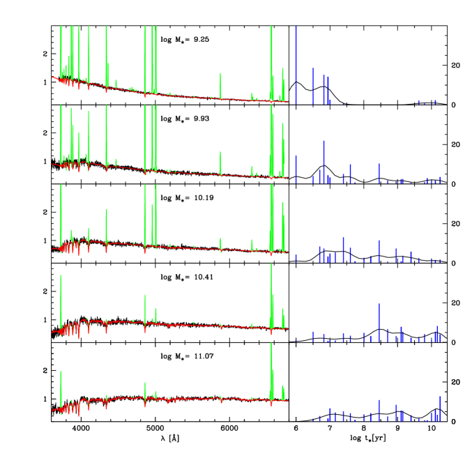
Figure 1: Five examples of the spectral fits. Left panels show the observed (black) and fitted (red) spectra, both normalized at $\lambda_{0}=4020$ Å. Magenta lines mark regions not used in the fits either because they contain emission lines or because of artifacts in the data. Middle panels illustrate the fraction of light at $\lambda_{0}$ associated to each of the 25 SSP ages used in the fits. Curves represent a 0.5 dex smoothed version of the population vector. Right panels show SDSS $25.6^{\prime\prime}\times 25.6^{\prime\prime}$ images ($\sim$ $12\times 12$–$34\times 34$ kpc²). Galaxies in this plot are ordered according to their nebular metallicity ($Z_{neb}$; see Section 2.4). From top to bottom, $Z_{neb}=0.29$, 0.43, 0.61, 0.84 and 0.97 $Z_{\odot}$.

The data analysed in this work was extracted from the SDSS Data Release 5 (DR5; Adelman-McCarthy et al., 2007). This release contains data for 582471 objects spectroscopically classified as galaxies, from which we have found $\sim 1.6$ per cent of duplicates, that is, objects with multiple spectroscopic information in the parent galaxy catalog.

From the remaining 573141 objects we have selected our parent sample adopting the following selection criteria: $14.5\leq m_{r}\leq 17.77$ and $z\geq 0.002$. The magnitude range comes from the definition of the Main Galaxy Sample, whereas the lower redshift limit is used to avoid inclusion of intragalactic sources. The resulting sample contains 476931 galaxies, which corresponds to about 82 per cent of all galaxies with spectroscopic data gathered by SDSS and publicly available in the DR5. These limits imply a reduction by $\sim 17\%$ in the sample studied in SEAGal V.

2.1 STARLIGHT fits

After correcting for Galactic extinction (with the maps of Schlegel, Finkbeiner & Davis, 1998 and the reddening law of Cardelli, Clayton & Mathis, 1989, using $R_{V}=3.1$), the spectra were shifted to the rest-frame, resampled to $\Delta\lambda=1$ Å between 3400 and 8900 Å, and processed through the starlight spectral synthesis code described in SEAGal I and II.

starlight decomposes an observed spectrum in terms of a sum of simple stellar populations (SSPs), each of which contributes a fraction $x_{j}$ to the flux at a chosen normalization wavelength ($\lambda_{0}=4020$ Å). As in SEAGal II, we use a base of $N_{\star}=150$ SSPs extracted from the models of Bruzual & Charlot (2003, BC03), computed for a Chabrier (2003) initial mass function (IMF), “Padova 1994” evolutionary tracks (Alongi et al., 1993; Bressan et al., 1993; Fagotto et al., 1994a, b; Girardi et al., 1996), and STELIB library (Le Borgne et al., 2003). The base components comprise 25 ages between $t_{\star,j}=1$ Myr and 18 Gyr, and 6 metallicities, from $Z_{\star,j}=0.005$ to 2.5 solar. Bad pixels, emission lines and the NaD doublet are masked and left out of the fits. The emission line masks were constructed in a galaxy-by-galaxy basis, following the methodology outlined in SEAGal II and Asari (2006). starlight outputs several physical properties, such as the present-day stellar mass, stellar extinction, mean stellar ages, mean metallicities as well as full time dependent star formation and chemical evolution histories, which will be used in our analysis. Section 4.1 describes aspects of the code relevant to this work.

Fitting half a million spectra represented a massive computational effort, carried out in a network of over 100 computers spread over 3 continents and controlled by a specially designed PHP code. This huge d’atabase of spectral fits and related products, as well as starlight itself, are publicly available in a Virtual Observatory environment at www.starlight.ufsc.br (see Cid Fernandes et al., 2007, in prep.).

Examples of the spectral fits obtained for 5 star-forming galaxies are shown in Fig 1. We have ordered the galaxies according to their nebular metallicity ($Z_{neb}$), as defined in Section 2.4, to illustrate how spectral characteristics change along the $Z_{neb}$ sequence. Metal-poor galaxies (top) show blue spectra and strong emission lines in comparison to the redder spectra and weaker emission lines of galaxies with a metal-rich ISM (bottom). The middle panels in Fig 1 show the fractional contribution to the total flux at $\lambda_{0}=4020$ Å of simple stellar population (SSP) of age $t_{\star}$. These panels show that young stellar populations make a dominant contribution in galaxies with low $Z_{neb}$, whereas at higher nebular metallicities a richer blend of stellar ages is present.

2.2 Emission lines

2.2.1 General procedure

Emission lines were measured fitting gaussians to the residual spectra obtained after subtraction of the stellar light using an updated version of the line-fitting code described in SEAGal III. The main transitions used in this study are H$\beta$, [OIII]$\lambda 5007$, H$\alpha$ and [NII]$\lambda 6584$. In the next section these lines are used to define the sub-sample of star-forming galaxies which will be studied in this paper.

2.2.2 The special case of H$\beta$

We find that a zero level residual continuum is adequate to fit the emission lines, except for H$\beta$. Inspection of the spectral fits shows that the synthetic spectrum is often overestimated in the continuum around H$\beta$, creating a broad, $\sim 200$ Å wide absorption trough in the residual spectrum. This problem, which can hardly be noticed in Fig 1, becomes evident when averaging many residual spectra (see SEAGal V and Panter et al., 2007), and tends to be more pronounced for older objects. The comparison between STELIB stars and theoretical models presented by Martins et al. (2005) gives a clue to the origin of this problem. A close inspection of Fig 21 in their paper shows that the STELIB spectrum has an excess of flux on both sides of H$\beta$ when compared to the model spectrum. This suggests that the “H$\beta$ trough” is related to calibration issues in the STELIB library in this spectral range. This was confirmed by starlight experiments which showed that the problem disappears using the SSP spectra of González-Delgado et al. (2005, based on the Martins et al. 2005 library) or those constructed with the MILES library (Sanchez-Blazquez et al., 2006).

Though this is a low amplitude mismatch (equivalent width $\sim 3$ Å spread over $\sim 200$ Å), it makes H$\beta$ sit in a region of negative residual flux, so assuming a zero level continuum when fitting a gaussian may chop the base of the emission line, leading to an underestimation of its flux. To evaluate the magnitude of this effect we have repeated the H$\beta$ fits, this time adjusting the continuum level from two side bands (4770–4830 and 4890–4910 Å). On average, the new flux measurement are 2% larger than the ones with the continuum fixed at zero. The difference increases to typically 4% for objects with $W_{H\beta}<5$ Å, but $S/N>3$ in the line, and 7% for $W_{H\beta}<2$ Å. Noise in the side bands introduces uncertainties in the measurement of the flux, but at least it removes the systematic effect described above, so the new measurements should be considered as more accurate on average. We adopt these new H$\beta$ measurements throughout this work. Using the zero continuum measurements changes some of the quantitative results reported in this paper minimally, with no impact on our general conclusions.

2.3 Definition of the Star Forming Sample

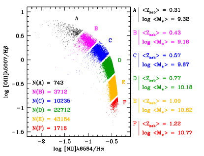
Figure 2: The SF sample in the BPT plane, chopped into bins of nebular abundance $Z_{\rm neb}=\frac{({\rm O/H})}{({\rm O/H})_{\odot}}$. All lines have been corrected by reddening (see Section 2.5). These same bins are used throughout this paper. The number of galaxies in each bin is given on the left. On the right, we show the corresponding mean $Z_{neb}$ and log mean $M_{\star}$ values (in solar units). Galaxies close to bin borders are not plotted for clarity.

Since the pioneering work of Baldwin, Phillips & Terlevich (1981), emission line objects are classified in terms of their location in diagrams involving pairs of line ratios. As explained in SEAGal III, the [NII]$\lambda 6584$/H$\alpha$ vs. [OIII]$\lambda 5007$/H$\beta$ diagram (the BPT diagram) is the most useful for this purpose, mainly due to the partially secondary nature of N (i.e., the increase of N/O as O/H increases, e.g., Liang et al., 2006; Mollá et al., 2006).

Our sample of star-forming galaxies is composed by objects which are below the line separating normal star-forming galaxies and AGN hosts proposed in SEAGal III. We have imposed a lower limit of 3 in $S/N$ on the 4 lines in the BPT diagram, and $S/N\geq 10$ in the 4730–4780 Å continuum to constitute our main sample (the SF sample). The 82302 galaxies composing the SF sample are shown in Fig. 2 on the BPT plane.

Both the starlight fits (and thus all SFH-related parameters) and the emission line data are affected by the quality of the spectra. To monitor this effect, we have defined a “high-quality” sub-set (the SF^hq sample) by doubling the $S/N$ requirements for the SF sample, i.e., $S/N\geq 6$ in all 4 lines in the BPT diagram and a continuum $S/N$ of 20 or better. A total of 17142 sources satisfy these criteria.

Fig. 3 shows the distributions of observational and physical properties for the samples. Naturally, the SF^hq sample is skewed towards closer and brighter galaxies with respect to the SF sample, but in terms of physical properties such as stellar mass, mean age and nebular metallicity the two samples are similar.

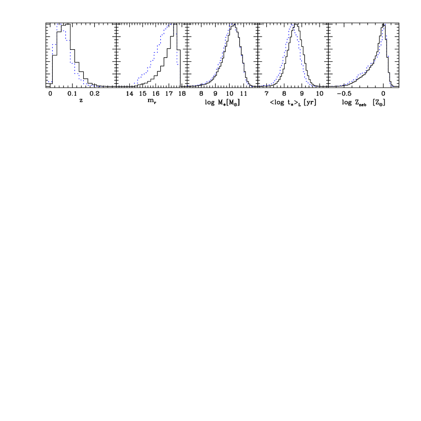
Figure 3: Normalized histograms of observed and physical properties for the SF (solid), SF^hq (dotted) samples.

2.4 Nebular Metallicity Estimate

It is well known that the SF-wing in the BPT diagram is a sequence in nebular metallicity (SEAGal III and references therein), which we quantify by the oxygen abundance obtained through the O₃N${}_{2}=$ [OIII]5007/[NII]6583 index as calibrated by Stasińska (2006):

$$\log Z_{neb}=\log\frac{{\rm(O/H)}}{{\rm~{}~{}(O/H)}_{\odot}}=-0.14-0.25\log{\rm O}_{3}{\rm N}_{2}$$ (1)

where we have adopted ${\rm(O/H)}_{\odot}=4.9\times 10^{-4}$ (Allende Prieto, Lambert & Asplund, 2001).

We have chosen to use the O₃N₂ indicator to estimate the average oxygen abundance in the ISM of SF galaxies mainly because it is a single-valued indicator and it can be easily related to the position of galaxies in the classical BPT diagram. However, this indicator is affected by the the presence of diffuse ionized gas in galaxies and by the fact that the N/O ratio depends on the way chemical evolution proceeded (Chiappini, Romano & Matteucci, 2003). In addition, for the lowest metallicity galaxies, O₃N₂ is not sensitive to O/H anymore, as a wide range of metallicities correspond to the same value of O₃N₂, as can be seen in Fig. 3 of Stasińska (2006). From that figure, the O/H given by equation (1) lies towards the upper end of the possible values of O/H. We considered using the [ArIII]7135/[OIII]5007 (Ar₃O₃) index which, as argued by Stasińska (2006), does not suffer from the problems mentioned for the O₃N₂ index. It turns out that, in objects where the [ArIII] line could be measured, Ar₃O₃ and O₃N₂ are extremely well correlated (with a Spearman correlation coefficient of $R_{S}=0.58$). Unfortunately, the quality of the SDSS spectra did not allow us to measure the [ArIII] line intensity with sufficient accuracy in a large number of objects, and principally in the zone where it would have been helpful to break the O₃N₂ vs O/H degeneracy. Using the Pilyugin & Thuan (2005) metallicity calibration based on [OIII]5007/H$\beta$ and [OII]3727/H$\beta$ adds only a tiny fraction of galaxies. The same applies when using the O/H values obtained by Izotov et al. (2006) from direct methods using the electron temperature derived from [OIII]4363/[OIII]5007. When comparing our measures with theirs, there is a systematic offset of 0.2 dex and a rms of 0.13 dex in $Z_{neb}$ for the 177 objects we have in common. This effect is greater the lower $Z_{neb}$ is. We thus decided to use O₃N₂ as a nebular metallicity indicator all along the SF galaxy sequence, keeping in mind that equation (1) will tend to attribute a metallicity $Z_{neb}$ of about 0.2 $Z_{\odot}$ for the galaxies with the lowest observed O₃N₂ in our sample.

Other metallicity estimates have been used for galaxies. For example, Tremonti et al. (2004) obtained the nebular metallicities by comparing the observed line ratios with a large data base of photoionization models. While a priori appealing, this method is not devoid of problems, as shown by Yin et al. (2007). There is a systematic offset of -0.28 dex and a rms of 0.09 between our nebular metallicities and theirs. Their method also yields a larger range of values for $Z_{neb}$. For the SF sample, their calibration covers from $Z_{neb}=0.78$ to 2.70 $Z_{\odot}$ for the 5 to 95 percentile ranges, whereas our calibration covers from 0.47 to 1.13 $Z_{\odot}$ for the same percentile ranges.

The calibration by Pettini & Pagel (2004) is more similar to our own. There is a slight offset of -0.04 dex with respect to our calibration and the dispersion for the SF sample is 0.03 dex. Their calibration also stretches a little the $Z_{neb}$ ranges: $Z_{neb}=0.45$ to 1.36 $Z_{\odot}$ for the 5 to 95 percentile ranges.

Although we believe that our calibration is likely more reliable, we have performed all the computations in this paper also with the Tremonti et al. (2004) and Pettini & Pagel (2004) calibrations. While the results differ in absolute scales, the qualitative conclusions remain identical.

2.4.1 $Z_{neb}$ bins

As seen above, both physical and mathematical motivations make O₃N₂ a convenient index to map galaxy positions along the SF wing in the BPT diagram. From equation (1) one sees that a given value of $Z_{neb}$ using this index defines a straight line of unit slope in the BPT diagram.

Our SF sample spans the $Z_{neb}=0.2$–1.6 $Z_{\odot}$ range from the tip of the SF-wing to its bottom. In Fig. 2 this interval is chopped into 6 bins of width $\Delta\log Z_{neb}=0.13$ dex, except for the one of lowest metallicity which is twice as wide to include more sources. Table 1 lists some properties of galaxies in each of these bins, which are hereafter labeled A–F. Galaxies inside these bins will be grouped together in the analysis of star-formation presented in Section 6. Note that the bias in the determination of $Z_{neb}$ from O₃N₂ at low metallicities has no consequence for our study, since almost all the objects from bin A remain in this bin.

	Bin A	Bin B	Bin C	Bin D	Bin E	Bin F
$\log Z_{neb}$ min [Z⊙]	-0.710	-0.450	-0.320	-0.190	-0.060	0.070
$\log Z_{neb}$ p05	-0.608	-0.435	-0.311	-0.180	-0.053	0.071
$\log Z_{neb}$ p50	-0.494	-0.364	-0.242	-0.111	-0.001	0.081
$\log Z_{neb}$ p95	-0.454	-0.324	-0.194	-0.064	0.054	0.112
$\log Z_{neb}$ max	-0.450	-0.320	-0.190	-0.060	0.070	0.200
$\log M_{\star}$ p05 [M⊙]	7.146	7.938	8.693	9.277	9.800	10.089
$\log M_{\star}$ p50	8.319	8.922	9.452	9.958	10.460	10.678
$\log M_{\star}$ p95	9.313	9.634	10.083	10.646	11.073	11.154
$\langle\log t_{\star}\rangle_{L}$ p05 [yr]	6.755	7.428	7.695	7.915	8.127	8.167
$\langle\log t_{\star}\rangle_{L}$ p50	7.762	8.155	8.385	8.567	8.726	8.724
$\langle\log t_{\star}\rangle_{L}$ p95	8.556	8.900	9.139	9.255	9.276	9.255
$\log L_{H\alpha}$ p05 [L⊙]	5.167	5.139	5.492	5.988	6.551	6.956
$\log L_{H\alpha}$ p50	6.475	6.475	6.750	7.149	7.544	7.816
$\log L_{H\alpha}$ p95	7.834	7.736	7.961	8.172	8.426	8.559
$\log b$ p05	-0.157	-0.392	-0.698	-0.947	-0.973	-0.890
$\log b$ p50	0.769	0.436	0.211	-0.006	-0.213	-0.199
$\log b$ p95	1.527	1.192	0.905	0.644	0.366	0.272

Table 1: Statistics of properties in bins A–F.

2.5 Extinctions

2.5.1 Stellar extinction

As explained in SEAGal I, starlight also returns an estimate of the stellar visual extinction, $A_{V}^{\star}$, modeled as due to a foreground dust screen. This is obviously a simplification of a complex problem (Witt, Thronson Jr. & Capuano Jr., 1992), so that $A_{V}$ should be called a dust attenuation parameter instead of extinction, although we do not make this distinction. Previous papers in this series have used the Cardelli, Clayton & Mathis (1989, CCM) reddening law, with $R_{V}=3.1$. In order to probe different recipes for dust attenuation, we have selected 1000 galaxies at random from the SF^hq sample and fitted them with four other functions: the starburst attenuation law of Calzetti, Kinney & Storchi-Bergmann (1994), the SMC and LMC curves from Gordon et al. (2003) and the $\lambda^{-0.7}$ law used by Kauffmann et al. (2003a).

We find that the quality of the spectral fits remains practically unchanged with any of these 5 laws. Averaging over all galaxies the SMC law yields slightly better $\chi^{2}$’s, followed closely by the Calzetti, $\lambda^{-0.7}$, LMC, and CCM, in this order. As expected, these differences increase with the amount of dust, as measured by the derived $A_{V}^{\star}$ values or by H$\alpha$/H$\beta$. Yet, KS-tests showed that in no case the distributions of $\chi^{2}$’s differ significantly. This implies that the choice of reddening law cannot be made on the basis of fit quality. A wider spectral coverage would be needed for a definitive empirical test.

When using different recipes for the dust attenuation, the synthesis algorithm has to make up for the small variations from one curve to another by changing the population vector and the value of $A_{V}^{\star}$. To quantify these changes we compare results obtained with the Calzetti and CCM curves, and consider only the most extincted objects. Compared to the results for a CCM law, with the Calzetti law the mean stellar age decreases by 0.09 dex on the median (qualitatively in agreement with the results reported in Fig 6 of Panter et al., 2007), the mean stellar metallicity increases by 0.05 dex, $A_{V}^{\star}$ increases by 0.07 mag and stellar masses decrease by 0.02 dex. These differences, which are already small, should be considered upper limits, since they are derived from the most extincted objects. Somewhat larger differences are found when using the SMC and $\lambda^{-0.7}$ laws. For instance, compared to the Calzetti law, the SMC law produces mean stellar ages 0.15 dex younger and masses 0.07 dex smaller, again for the most extincted objects.

We have opted to use the Calzetti law in our starlight fits and emission line analysis. The reasons for this choice are twofold: (1) The Calzetti law yields physical properties intermediate between the SMC and CCM laws, and (2) this law was built up on the basis of integrated observations of SF galaxies, similar to the ones studied in this paper. In any case, the experiments reported above show that this choice has little impact upon the results.

starlight also allows for population dependent extinctions. Although tests with these same 1000 galaxies sample show that in general one obtains larger $A_{V}^{\star}$ for young populations, as expected, simulations show that, as also expected, this more realistic modeling of dust effects is plagued by degeneracies which render the results unreliable (see also Panter et al., 2007; SEAGal V). We therefore stick to our simpler but more robust single $A_{V}^{\star}$ model.

2.5.2 Nebular extinction

The nebular V-band extinction was computed from the H$\alpha$/H$\beta$ ratio assuming a Calzetti et al. (1994) law:

$$A_{V}^{neb}=7.96\log{\rm\frac{(H\alpha/H\beta)_{obs}}{(H\alpha/H\beta)_{int}}}$$ (2)

where ${\rm(H\alpha/H\beta)_{obs}}$ and ${\rm(H\alpha/H\beta)_{int}}$ are the observed and intrinsic ratio respectively. Instead of assuming a constant value, we take into account the metallicity dependence of ${\rm(H\alpha/H\beta)_{int}}$, which varies between 2.80 and 2.99 for $Z_{neb}$ in the 0.1 to 2.5 $Z_{\odot}$ range, as found from the photoionization models in SEAGal III.

We obtain the intrinsic ratio as follows. We start by assuming ${\rm(H\alpha/H\beta)_{int}}=2.86$, from which we derive a first guess for $A_{V}^{neb}$. We then use the dereddened ${\rm[OIII]}\lambda 5007$ and ${\rm[NII]}\lambda 6584$ line fluxes to calculate $Z_{neb}$ (eq. 1). From our sequence of photoionization models (SEAGal III) and $Z_{neb}$, we derive a new estimate for ${\rm(H\alpha/H\beta)_{int}}$, and hence $A_{V}^{neb}$ (eq. 2). It takes a few iterations (typically 2–3) to converge.

For 1.6% of the objects (1.1% for the SF^hq sample), H$\alpha$/H$\beta$ is smaller than the intrinsic value, which leads to $A_{V}^{neb}<0$. In such cases, we assume $A_{V}^{neb}=0$. We have corrected both the [OIII]/H$\beta$ and [NII]/H$\alpha$ line ratios for dust attenuation for the remainder of our analysis.

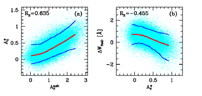
Figure 4: (a) Relation between stellar and nebular extinctions for the SF sample. Lines indicate the 5, 50 and 95 percentiles. (b) Equivalent width of the ISM component of the NaD doublet (as measured from residual spectra) against the stellar extinction.

We find that $A_{V}^{neb}$ and $A_{V}^{\star}$ are strongly correlated, as shown in Fig 4a. A robust linear fit including all points yields $A_{V}^{neb}=0.34+2.28A_{V}^{\star}$. The ionized gas thus suffers $\sim$ twice as much extinction as the stellar continuum, corroborating the results reported in Stasińska et al. (2004) (with a different methodology) and SEAGal I (obtained with a smaller sample, different version of starlight and a CCM extinction curve), and in agreement with detailed studies of nearby SF-galaxies (Calzetti et al., 1994). We also find that the difference between nebular and stellar extinctions increases systematically as the mean age of the stellar population increases.

Given the spatial association of the line emitting gas and the ionizing populations, these results ultimately imply a breakdown of our simple single-$A_{V}^{\star}$ modelling. In fact, starlight experiments with population dependent $A_{V}^{\star}$ point in the same direction, i.e, the need to allow young populations to suffer more extinction than older ones. To evaluate to which extent this simplification affects the results reported in this paper, Sec. 7.3 presents experiments where the extinction of $t_{\star}\leq 10$ Myr components is set according to the empirical relation $A_{V}^{neb}(A_{V}^{\star})$ found above.

2.5.3 Interstellar absorption as traced by the NaD doublet

The most conspicuous spectroscopic feature of the cold ISM in the optical range is the NaD doublet at $\lambda\lambda$5890,5896 Å. For a constant gas to dust ratio, the strength of this feature, which measures the amount of cold gas in front of the stars, should correlate with $A_{V}^{\star}$, as found for far-IR bright starburst galaxies (Heckman et al., 2000). To perform this test for our sample, we first measure the flux of the NaD doublet in the residual spectrum, integrating from 5883 to 5903 Å. We thus remove the stellar component of this feature, which is also present in stellar atmospheres, particularly late type stars (Jacoby, Hunter & Christian, 1984; Bica et al., 1991). In principle, this is a more precise procedure than estimating the stellar NaD from its relation to other stellar absorption lines (Heckman et al., 2000; Schwartz & Martin, 2004), but since the NaD window was masked in all fits (precisely because of its possible contamination by ISM absorption), the stellar NaD predicted by the fits rely entirely on other wavelengths, so in practice this is also an approximate correction. The residual flux is then divided by the continuum in this range (defined as the median synthetic flux in the 5800–5880 plus 5906-5986 Å windows), yielding the excess equivalent width $\Delta W_{\rm NaD}$, which says how much stronger (more negative) the NaD feature is in the data with respect to the models.

Fig 4b shows the relation between $\Delta W_{\rm NaD}$ and $A_{V}^{\star}$. The plot shows that these two independently derived quantities correlate strongly. Intriguingly, $\Delta W_{\rm NaD}$ converges to $0.8$ Å in the median as $A_{V}^{\star}\rightarrow 0$. We interpret this offset from $\Delta W_{\rm NaD}=0$ as due to the fact that the stars in the STELIB library have a Galactic ISM component in their NaD lines. This propagates to our spectral models, leading to an overprediction of the stellar NaD strength, and thus $\Delta W_{\rm NaD}>0$ when the ISM absorption approaches zero.

Regardless of such details, the discovery of this astrophysically expected correlation strengthens the confidence in our analysis. Furthermore, it opens the interesting prospect of measuring the gas-to-dust ratio and study its relation with all other galaxy properties at hand, from nebular metallicities to SFHs. This goes beyond the scope of the present paper, so we defer a detailed analysis to a future communication.

3 Correlations with nebular metallicity

Galaxy properties change substantially from the tip of the SF-wing, where small, metal-poor HII-galaxy-like objects live, to its bottom, populated by massive, luminous galaxies with large bulge-to-disk ratios and rich in metals (Kennicutt, 1998). The simplest way to investigate these systematic trends is to correlate various properties with the nebular metallicity (e.g., Tremonti et al., 2004; Brinchmann et al., 2004).

In this section we correlate $Z_{neb}$ with both observed and physical properties extracted from our stellar population fits. This traditional analysis, based on current or time-averaged properties, helps the interpretation of the more detailed study of time-dependent SFHs presented in the next sections. In fact, this is the single purpose of this section. Since most of the results reported in this section are already know or indirectly deducible from previous work, we will just skim through these correlations.

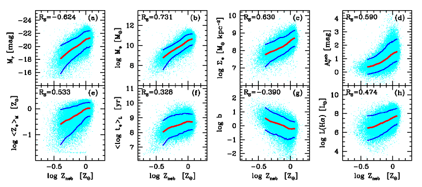
Figure 5: Correlations of $Z_{neb}$ and (a) the absolute r-band magnitude, (b) the stellar mass, (c) the surface mass density, (d) the nebular extinction, (e) the mean stellar metallicity, (f) the mean stellar age, (g) the ratio of current to mean past SFR, and (h) the H$\alpha$ luminosity. Numbers in each panel report the Spearman rank correlation coefficient, and the lines mark the 5, 50 and 95% percentiles of 25 bins, 3292 points in each bin. The right hand scale in panel (h) is also $\log L_{H\alpha}$, but in units of $2\times 10^{8}L_{\odot}$, such that it can also be read as an estimate of the current SFR in $M_{\odot}\,$yr^-1 (Section 5).

Fig 5a shows $Z_{neb}$ against absolute r-band magnitude. This is the luminosity-nebular metallicity relation, previously studied by many authors, and interpreted in terms of a mass-metallicity relation. Fig 5b shows our version of the $M_{\star}$–$Z_{neb}$ relation. Because of the expected bias in our $Z_{neb}$ estimate at the lowest metallicities (see Section 2.4), we expect the real mass-metallicity relation to be flatter at low $M_{\star}$ than seen in this plot.

As shown by Kauffmann et al. (2003b), stellar mass and stellar surface mass density ($\Sigma_{\star}$) are very strongly related. It is thus no surprise to find that $\Sigma_{\star}$ also correlates with $Z_{neb}$, as shown in Fig 5c. Our definition of $\Sigma_{\star}$ is the same as adopted by Kauffmann et al. (2003b), namely $\Sigma_{\star}=M_{\star}/2\pi r_{50,z}^{2}$, where $r_{50,z}$ is the half light Petrosian radius in the z-band.

Fig 5d shows how nebular extinction increases systematically with $Z_{neb}$. One factor which surely contributes to this relation is the rise in dust grain formation with increasing gas metallicity, but other factors may come into play as well (Stasińska et al., 2004).

Fig 5e shows how nebular and stellar metallicities correlate. This important relation, first presented in SEAGal I (for different sample, SSP base and $Z_{neb}$ scale), shows that stellar and ISM chemical enrichment levels scale with each other, as one would expect on the basis of simple chemical evolution scenarios. The large scatter in Fig 5e is mostly intrinsic (as we verified comparing the relation obtained for data of different qualities), in qualitative agreement with the idea that stellar and nebular metallicities reflect different evolutionary phases and react differently to the several processes which regulate the chemical evolution of galaxies. A similar relation was obtained by Gallazzi et al. (2005) using different methods to estimate both stellar and nebular abundances. Even though we express both quantities in solar units, these two metallicities are derived by such radically different means that, as discussed in SEAGal V, they should not be compared in quantitative terms.

The relation between the mean stellar age $\langle\log t_{\star}\rangle_{L}$ and $Z_{neb}$, shown in Fig 5f, reflects the fact that young stars have a larger share of the light output at the tip of the SF wing than at its bottom, where old populations have a greater weight. Metal-rich SF galaxies thus have a more continuous star-forming history than metal-poor ones, which are often dominated (in light, but not mass) by the latest generation of stars (e.g., Corbin et al., 2006). This is another way to look at metallicity–age trend, discussed previously in the analysis of Fig. 1. Ultimately, this relation represents a summary of chemical evolution, in the sense that more evolved systems have a more enriched ISM. In a related vein, Fig 5g shows how the ratio of current to mean past SFR (defined in Section 5.3) varies along the metallicity sequence of SF galaxies. This indicates that the lower-metallicity galaxies are slower in forming stars. When one considers the mass-metallicity relation (Fig 5b), this is just another way of looking at the downsizing effect (Heavens et al., 2004; Thomas et al., 2005; Mateus et al., 2006). Finally, Fig 5h shows the relation between reddening corrected H$\alpha$ luminosity and $Z_{neb}$. The y-axis is given in units such that the values correspond $\sim$ to the current SFR in $M_{\odot}\,$yr^-1 (see Section 5). The correlation, although statistically unquestionable, has a large scatter. This implies that galaxies in the 6 $Z_{neb}$ bins defined in Fig 2 have heavily overlapping current SFRs. Section 6 presents independent confirmation of this fact.

As expected, all correlations discussed above are also present for the SF^hq sub-sample. For most they are in fact somewhat stronger, whereas for samples defined with less stringent criteria the correlation strengths weaken, indicating that noise in the data is responsible for part of the scatter in these relations. Finally, as is widely known and can be deduced from Fig 5 itself, there are many inter-relations between galaxy properties. Our use of $Z_{neb}$ as the “independent” variable axis in Fig 5 is not meant to indicate that $Z_{neb}$ is the underlying cause of the correlations; it simply reflects our interest in mapping physical properties of galaxies along the SF wing of the seagull in the BPT diagram.

4 Methods to investigate star formation histories

The main goal of this paper is to study how the SFH varies among SF galaxies. Most other investigations in this same line used absorption, emission or continuum spectral indices such as the 4000 Å break, the H$\delta$ absorption, the K, G and Mg bands, or the H$\alpha$ luminosity and equivalent widths to characterize the SFH (e.g., Raimann et al., 2000; Kong et al., 2003; Kauffmann et al., 2003b; Cid Fernandes et al., 2003; Brinchmann et al., 2004; Westera et al., 2004). Our approach, instead, is to infer the SFH from detailed pixel-by-pixel fits to the full observed spectrum, thus incorporating all available information.

Whereas our previous work concentrated on the first moments of the age and metallicity distributions, here we present some basic formalism towards a robust description of SFHs as a function of time. From the point of view of methodology, these may be regarded as “second-order” products. Astrophysically, however, recovering the SFH of galaxies is of prime importance. SEAGal V presented our first results in this direction, including empirically derived time-dependent mean stellar metallicities. In this section we expand upon these results, exploring new ways to handle the output of the synthesis, focusing of the SFHs.

4.1 Compression methods

As reviewed in Section 2.1, starlight decomposes an observed spectrum in terms of a sum of SSPs, estimating the $x_{j}$ ($j=1\cdots N_{\star}$) fractional contribution of each population to the flux at $\lambda_{0}=4020$ Å. For this work we used a base of $N_{\star}=150$ SSPs from BC03, spanning 25 ages between $t_{\star,j}=1$ Myr and 18 Gyr, and 6 metallicities ($0.005\leq Z_{\star,j}\leq 2.5Z_{\odot}$). Example fits were shown in Fig 1.

Not surprisingly, the 150 components of the population vector ($\vec{x}$) are highly degenerate due to noise, and astrophysical plus mathematical degeneracies, as confirmed by simulations in Cid Fernandes et al. (2004) and SEAGal I. These same simulations, however, proved that compressed versions of the population vector are well recovered by the method.

Different compression approaches exist among spectral synthesis codes. In MOPED (Heavens, Jimenez & Lavah, 2000; Reichardt et al., 2001; Panter et al., 2003; Panter et al., 2007; Heavens et al., 2004), for instance, compression is done a priori, replacing the full spectrum by a set of numbers associated to each of the $N_{\star}+1$ parameters (the mass fractions and metallicities in several time bins plus a dust parameter). STECMAP (Ocvirk et al., 2006) performs a compression by requiring the resulting SFH to be relatively smooth. The preference for a smooth solution over a ragged one is effectively a prior, but the algorithm adjusts the degree of smoothing in a data driven fashion, so we may call it an “on the fly” compression method. The same can be said about VESPA (Tojeiro et al., 2007), a new code which combines elements from these two approaches. starlight is less sophisticated in this respect. Its only built-in compression scheme is that the final stages of the fit (after the Markov Chains reach convergence) are performed with a reduced base comprising the subset of the original $N_{\star}$ populations which account for $\geq 99\%$ of the light. For our parent sample of 573141 galaxies the average size of this subset is $\overline{N_{\star}^{\rm eff}}=24$ populations, while for the 82302 galaxies in the SF sample $\overline{N_{\star}^{\rm eff}}=41$. (This difference happens because the full sample has many old, passive systems, which require relatively few SSPs, whereas SF galaxies have more continuous SF regimes, thus requiring more SSPs to be adequately fit.) Compression beyond this level must be carried out a posteriori by the user. As explained in the next section, in this study we in fact compress this information into only four age bins by smoothing the population vectors.

Previous papers in this series have taken this a posteriori compression approach to its limit, condensing the whole age distribution to a single number, the mean stellar age:

$$\langle\log t_{\star}\rangle_{L}=\sum_{j=1}^{N_{\star}}x_{j}\log t_{\star,j}$$ (3)

where the subscript $L$ denotes a light-weighted average. Mass-weighted averages are readily obtained replacing $\vec{x}$ by the mass-fraction vector $\vec{\mu}$. Similarly, stellar metallicities were only studied in terms of their mass-weighted mean value:

$$\langle Z_{\star}\rangle_{M}=\sum_{j=1}^{N_{\star}}\mu_{j}Z_{\star,j}$$ (4)

Simulations show that both of these quantities have small uncertainties and essentially no bias. Regarding practical applications, these first moments proved useful in the study of several astrophysical relations, some of which have just been presented in Section 3 (see Fig. 5). Notwithstanding their simplicity, robustness and usefulness, these averages throw away all time dependent information contained in the population vector, thus hindering more detailed studies of galaxy evolution. In what follows we explore novel ways to deal with the population vector which circumvent this limitation.

4.2 Star Formation Rate as a Function of Time

One alternative to characterize higher moments of the SFH is to bin $\vec{x}$ onto age-groups, a strategy that goes back to Bica (1988; see also Schmidt et al., 1991; Cid Fernandes et al., 2001). Though useful, this approach introduces the need to define bin-limits, and produces a discontinuous description of the SFH.

A method which circumvents these disadvantages is to work with a smoothed version of the population vector. We do this by applying a gaussian filter in $\log t_{\star}$, with a FWHM of 1 dex. Given that our base spans $\sim 4$ orders of magnitude in $t_{\star}$, this heavy smoothing is equivalent to a description in terms of $\sim 4$ age groups, but with the advantage that $\vec{x}_{s}$ can be sampled continuously in $\log t_{\star}$. This approach is analogous to smoothing a noisy high-resolution spectrum to one of lower resolution, but whose large-scale features (colours, in this analogy) are more robust. From the results in SEAGal I, where it was shown that 3 age groups are reliably recovered, we expect this smoothing strategy to be a robust one. Furthermore, averaging over a large number of objects minimizes the effects of uncertainties in the smoothed SFH for individual galaxies.

Technically, the issue of age resolution in population synthesis is a complex one. Ocvirk et al. (2006), for instance, find that bursts must be separated by about 0.8 dex in $\log t_{\star}$ to be well distinguished from one another with their SFH inversion method. Considering that the age range spanned by our base is 4.2 dex wide, one obtains 5 “independent” time bins. This number is similar to that (6 bins) used by Mathis, Charlot & Brinchmann (2006) to describe the SFH of SDSS galaxies (covering a wider $\lambda$-range than those simulated by Ocvirk et al. but at lower S/N) with a variant of the MOPED code. Up to 12 time bins were used in other applications of MOPED. Panter et al. (2007) argue that this may be a little too ambitious for individual galaxies, but uncertainties in this overparameterized description average out in applications to large samples. Tojeiro et al. (2007) have a useful discussion on the number of parameters that can be recovered with synthesis methods. By using their VESPA code and calculating the number of parameters on the fly for each individual object, they find that tipically 2–8 parameters can be robustely recovered for SDSS spectra. Hence, despite the complexity of the issue, there seems to be some general consensus that the age resolution which can be achieved in practice is somewhere between 0.5 and 1 dex, so our choice of smoothing length is clearly on the conservative side.

A further advantage of this continuous description of the SFH is that it allows a straight-forward derivation of a star-formation rate (SFR). Recall that we describe a galaxy’s evolution in terms of a succession of instantaneous bursts, so a SFR is not technically definable unless one associates a duration to each burst. The ${\rm SFR}(t_{\star})$ function is constructed by sampling the smoothed mass-fraction vector $\vec{\mu}^{c}_{s}$ in a quasi-continuous grid from $\log t_{\star}=5.6$ to 10.5 in steps of $\Delta\log t_{\star}=0.1$ dex, and doing

$${\rm SFR}(t_{\star})=\frac{dM^{c}_{\star}(t_{\star})}{dt_{\star}}\approx\frac{\Delta M^{c}_{\star}(t_{\star})}{\Delta t_{\star}}=\frac{M_{\star}^{c}\log e}{t_{\star}}\frac{\mu^{c}_{s}(t_{\star})}{\Delta\log t_{\star}}$$ (5)

where $M_{\star}^{c}$ is the total mass converted to stars over the galaxy history until $t_{\star}=0$, and $\vec{\mu}^{c}_{s}(t_{\star})$ is the fraction of this mass in the $t_{\star}$ bin.

We can also define the time dependent specific SFR:

$${\rm SSFR}(t_{\star})=\frac{1}{M^{c}_{\star}}\frac{dM^{c}_{\star}(t_{\star})}{dt_{\star}}\approx\frac{\log e}{t_{\star}}\frac{\mu^{c}_{s}(t_{\star})}{\Delta\log t_{\star}}$$ (6)

which measures the pace at which star-formation proceeds with respect to the mass already converted into stars. This is a better quantity to use when averaging the SFH over many objects, since it removes the absolute mass scale dependence of equation (5).

Three clarifying remarks are in order. (1) All equations above are marginalized over $Z_{\star}$, i.e., ${\rm SFR}(t_{\star})=\sum_{Z_{\star}}{\rm SFR}(t_{\star},Z_{\star})$ measures the rate at which gas is turned into stars of any metallicity. (2) The upper age limit of our base (18 Gyr) is inconsistent with our adopted cosmology, which implies an 13.5 Gyr Universe. Given the uncertainties in stellar evolution, cosmology, observations and in the fits themselves, this is a merely formal inconsistency, and, in any case, components older than 13.5 Gyr can always be rebinned to a cosmologically consistent time grid if needed. (3) Finally, since our main goal is to compare the intrinsic evolution of galaxies in different parts of the SF wing in the BPT diagram, throughout this paper we will consider ages and lookback times in the context of stellar-evolution alone. In other words we will not translate $t_{\star}$ to a cosmological lookback time frame, which would require adjusting the $t_{\star}$ scale by adding the $z$-dependent lookback time of each galaxy.

4.3 Mass Assembly Histories

Another way to look at the population vector is to compute the total mass converted into stars as a function of time:

$$\eta^{c}_{\star}(t_{\star})=\sum_{t_{\star,j}>t_{\star}}\mu^{c}_{j}$$ (7)

which is a cumulative function that grows from 0 to 1, starting at the largest $t_{\star}$, tracking what fraction of $M^{c}_{\star}$ was converted to stars up to a given lookback time.

We sample $\eta^{c}_{\star}$ in the same $\log t_{\star}=5.6$–10.5 grid used to describe the evolution of the SFR, but here we operate on the original population vector, not the smoothed one. Since most of the mass assembly happens at large $t_{\star}$, computing $\eta^{c}_{\star}$ with the smoothed SFHs leads to too much loss of resolution. In essence, however, $\eta^{c}_{\star}(t_{\star})$ and ${\rm SSFR}_{\star}(t_{\star})$ convey the same physical information in different forms.

5 The current SFR

The most widely employed method to measure the “current” SFR is by means of the H$\alpha$ luminosity (Kennicutt, 1983, 1998; Hopkins et al., 2003). We have just devised ways of measuring the time dependent SFR which rely exclusively on the stellar light, from which one can define a current SFR averaging over a suitably defined time interval. Before proceeding to the application of these tools to study the detailed SFHs of galaxies, this section compares these two independent methods to estimate the current SFR.

The purpose of this exercise is three-fold. First, it serves as yet another sanity check on the results of the synthesis. Secondly, it allows us to define in an objective way the ratio of current to past-average SFR, often referred to as Scalo’s $b$ parameter (Scalo, 1986), which is a useful way to summarize the SFH of galaxies (e.g., Sandage, 1986; Brinchmann et al., 2004). Finally, defining and calibrating a synthesis-based measure of current SFR equivalent to that obtained with H$\alpha$, allows one to estimate the current SFR in galaxies where H$\alpha$ is not powered exclusively by young stars. This turns out to be very useful in studies of AGN hosts (Torres-Papaqui et al., 2007, in prep.).

5.1 Current SFR from H$\alpha$ luminosity

For a SFR which is constant over times-scales of the order of the lifetime of massive ionizing stars ($t_{ion}\sim 10$ Myr), the rate of H-ionizing photons converges to

$$Q_{H}={\rm SFR}\,{\cal N}_{H}({\rm IMF},Z_{\star})$$ (8)

where ${\cal N}_{H}$ is the number of $h\nu>13.6$ eV photons produced by a SSP of unit mass over its life (in practice, over 95% of the ionizing radiation is produced in the first 10 Myr of evolution). We computed ${\cal N}_{H}$ by integrating the $Q_{H}(t)$ curves for SSPs using the tables provided by BC03, obtaining ${\cal N}_{H}=9.12$, 7.08, 6.17, 5.62, 4.47 and $3.16\times 10^{60}$ photons M${}_{\odot}^{-1}$ for $Z_{\star}=0.005$, 0.02, 0.2, 0.4, 1 and 2.5 $Z_{\odot}$, respectively, for a Chabrier (2003) IMF between 0.1 and 100 M_⊙.

One in every 2.226 ionizing photons results in emission of an H$\alpha$ photon, almost independently of nebular conditions (Osterbrock & Ferland, 2006). This assumes Case B recombination and that no ionizing photon escapes the HII region nor is absorbed by dust. Adopting the Chabrier IMF and the $Z_{\odot}$ value of ${\cal N}_{H}$ leads to:

$${\rm SFR}_{H\alpha}=\frac{2.226L_{H\alpha}}{{\cal N}_{H}h\nu_{H\alpha}}=2M_{\odot}yr^{-1}\left(\frac{L_{H\alpha}}{10^{8}L_{\odot}}\right)$$ (9)

This calibration is strongly dependent on the assumed IMF and upper stellar mass limit. Given its reliance on the most massive stars, which comprise a tiny fraction of all the stars formed in a galaxy, SFR_Hα involves a large IMF-dependent extrapolation, and thus should be used with care.

5.2 Current SFR from the spectral synthesis

The SFR from spectral synthesis is based on all stars that contribute to the visible light, and thus should be more representative of the true SFR. We define a mean “current” SFR from our time dependent SFHs using equation (7) to compute the mass converted into stars in the last $\tau$ years, such that

$$\overline{{\rm SFR}_{\star}}(\tau)=M_{\star}^{c}\frac{1-\eta^{c}_{\star}(\tau)}{\tau}$$ (10)

is the mean SFR over this period. Because of the discrete nature of our base, the function $\overline{{\rm SFR}_{\star}}(\tau)$ has a “saw-tooth” appearance, jumping every time $\tau$ crosses one of the $t_{\star,j}$’s bin borders.

For the reasons discussed in Section 4.1, it is desirable to include components spanning $\sim 1$ dex in age to obtain robust results. Since our base starts at 1 Myr, $\tau\sim 10$ Myr would be a reasonable choice. This coincides with the minimum time-scale to obtain $\overline{{\rm SFR}_{\star}}(\tau)$ estimates comparable to those derived from $L_{H\alpha}$, which are built upon the assumption of constant SFR over $\tau\geq t_{ion}\sim 10$ Myr. Our base ages in this range are $t_{\star,j}=10$, 14, 25, 40 and 55 Myr.

5.3 Synthesis versus H$\alpha$-based current SFRs

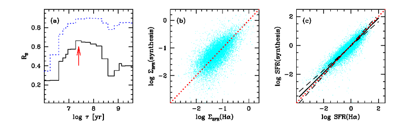
Figure 6: (a) The solid line shows the Spearman coefficient ($R_{S}$) of the $\Sigma_{SFR}({\rm synthesis})\times\Sigma_{SFR}(H\alpha)$ correlation for different values of $\tau$ in equation (10). The dotted line indicates the strength of the ${\rm SFR}({\rm synthesis})\times{\rm SFR}(H\alpha)$ correlation. (b) Correlation between the SFR per unit area obtained through H$\alpha$ and our synthesis (for $\tau=24.5$ Myr). Units are $M_{\odot}\,yr^{-1}\,kpc^{-2}$ for both axis. The dotted line marks the identity line. (c) Correlation between the SFRs derived from equations (10) and (9). Dashed lines indicate the $y(x)$ and $x(y)$ linear regressions, while the solid line shows the bisector fit.

To compare the SFRs given by equations (9) and (10) we must first choose a specific value for $\tau$. We do this by correlating the SFR per unit area obtained with these two estimators, and seeking the value of $\tau$ which yields the best correlation. Surface densities were used to remove the $d^{2}$ factors common to both SFRs, thus avoiding distance-induced correlations. Data for the SF^hq sample was used in this calibration. Also, since $L_{H\alpha}$ refers to the emission from within the $3^{\prime\prime}$ SDSS fibers, $M^{c}_{\star}$ was not extrapolated to the whole galaxy in this comparison.

Fig. 6 shows the results of this exercise. Panel a shows the run of the Spearman coefficient ($R_{S}$) for different values of $\tau$, with the best value indicated by an arrow. Given the discreteness of our base, any value in the range of the $t_{\star}=25$ Myr bin yield identically strong correlations (i.e., same $R_{S}$). We chose $\tau=24.5$ Myr because this value yields zero offset between these two SFRs. This is not a critical choice, as values in the whole 10 to 100 Myr range yield correlations of similar strength (Fig. 6a). The corresponding correlations between the synthesis and H$\alpha$-based SFRs are shown in panels b and c in terms of SFR surface densities and absolute SFRs, respectively. Robust fits to these relations yield slopes very close to unity (1.09 in Fig. 6b and 0.94 in Fig. 6c).

The rms difference between these two SFR estimators is 0.3 dex, corresponding to a factor of 2. We consider this an excellent agreement, given that these estimators are based on entirely different premises and independent data, and taking into account the uncertainties inherent to both estimators. It is also reassuring that $\tau$ turns out to be comparable to $t_{ion}\sim 10$ Myr, which is (by construction) the smallest time-scale for SFR_Hα to be meaningful. That the scatter between SFR_Hα and ${\rm SFR}_{\star}$ is typically just a factor of two can be attributed to the fact that we are dealing with integrated galaxy data, thus averaging over SF regions of different ages and emulating a globally constant SFR, which works in the direction of compatibilizing the hypotheses underlying equations (9) and (10).

With these results, we define the ratio of “current” to mean past SFR as

$$b=\frac{\overline{{\rm SFR}_{\star}}(\tau=24.5{\rm Myr})}{\overline{{\rm SFR}_{\star}}(\tau=\tau_{G})}$$ (11)

where $\tau_{G}$ is the age of the oldest stars in a galaxy. In practice, since the overwhelming majority of galaxies contain components as old as our base allows, the denominator is simply $M_{\star}^{c}$ divided by the age of the Universe, such that $b$ is ultimately a measure of the current specific SFR. This definition was used in Section 3, where its was shown that $b$ decreases by an order of magnitude in the median from the top to the bottom of the SF-wing.

6 The Star Formation Histories of SF Galaxies

Spectral synthesis methods such as the one employed in this work have historically been seen with a good deal of skepticism, best epitomized by Searle (1986), who, when talking about the spectral synthesis of integrated stellar populations, said that “too much has been claimed, and too few have been persuaded”. Persuading the reader that one can nowadays recover a decent sketch of the time-dependent SFR in a galaxy from its spectrum requires convincing results. In this section we apply the new tools to describe SFHs presented above (equations 5 to 7) to SF-galaxies in the SDSS. As shown below, the temporal-dimension leads to a more detailed view of SF-galaxies than that obtained with mean ages or current SFR estimates.

6.1 Distributions of Star Formation Histories

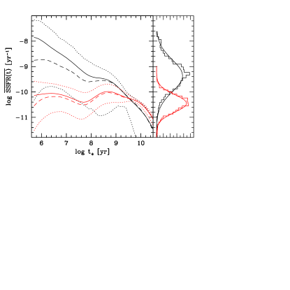
Figure 7: Left: Distributions of star formation histories for $Z_{neb}$-bins A (black) and F (red), as defined in Fig 2. For each bin, we show the mean SSFR (solid line), the median (dashed) and the 5 and 95 percentiles of the distributions (dotted). Right: Normalized distributions of log SSFR for $t_{\star}=25$ Myr. Gaussians are superimposed to illustrate that the distributions are log normal.

Our general strategy to explore the statistics of the sample is to group galaxies according to certain similarity criteria and derive mean SFHs for each group. Since all the results presented from Section 6.2 onwards are based on mean SFHs, it is fit to first ask how representative such means are of the whole distribution of SFHs.

This is done in Fig 7, where we show the full $t_{\star}$-by-$t_{\star}$ distribution of SSFR$(t_{\star})$, computed with equation (6), for two of the six bins in $Z_{neb}$ defined in Fig 2: bins A and F, plotted in black and red, and centered at $Z_{neb}=0.31$ and 1.22, respectively. Solid lines indicate the mean SSFR, dashed lines show the median and dotted lines the corresponding 5 and 95 percentiles of the distributions. The first thing one notices in this plot is that the distributions are very wide. For instance, for most of the $t_{\star}<1$ Gyr range, their 5 to 95 percentile ranges span over 2 orders of magnitude in SSFR. As discussed further below, this is in part due to the choice of grouping galaxies by $Z_{neb}$. Grouping by properties more directly related to the SFHs should lead to narrower distributions. However, one must realize that since galaxy evolution depends on many factors, grouping objects according to any single property will never produce truly narrow SFH distributions. Secondly, the distribution of SSFR values at any $t_{\star}$ is asymmetric, as can be seen by the fact that the mean and median curves differ. In fact, as illustrated by the right panel in Fig 7, these distributions are approximately log-normal, indicating that SFHs result from the multiplication of several independent factors, as qualitatively expected on physical grounds.

Despite their significant breadth and overlap, it is clear that the SSFR-distributions for $Z_{neb}$ bins A and F in Fig 7 are very different, particularly at low $t_{\star}$. This is confirmed by KS tests, which show that these two distributions are undoubtedly different. In fact, for any pair of $Z_{neb}$ bins the distributions differ with $>99\%$ confidence for any $t_{\star}$,

In what follows we will present only mean SFHs, obtained grouping galaxies according to a subset of the available physical parameters. Whilst their is clearly more to be learned from the SFH distributions discussed above, this is a useful first approach to explore the intricate relations between galaxy properties and their SFHs.

6.2 Trends along the SF-wing

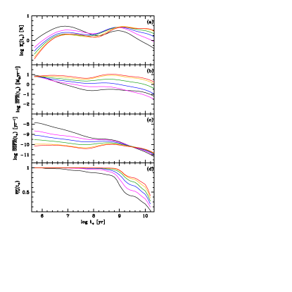
Figure 8: Mean star formation histories for the 6 different $Z_{neb}$-bins defined in Fig 2, in four different representations: (a) smoothed population vector, $\overline{x_{s}}(t_{\star})$, (b) $\overline{\rm SFR}(t_{\star})$, (c) $\overline{\rm SSFR}(t_{\star})$, and (d) $\overline{\eta^{c}_{\star}}(t_{\star})$.

We start our statistical study of galaxy SFHs grouping galaxies in the six $Z_{neb}$ bins defined in Section 2. As shown in Fig 2, $Z_{neb}$ traces the location of a galaxy along the SF-wing in the BPT diagram.

Fig 8 shows the derived SFHs for the A–F bins in four different representations, from top to bottom: $x_{s}$, SFR, SSFR and $\eta^{c}_{\star}$ as a function of stellar age $t_{\star}$. Each line represents a $t_{\star}$-by-$t_{\star}$ average over all galaxies in the bin. The plots show that young populations are present in a proportion which increases systematically as $Z_{neb}$ decreases. This is evident, for instance, in the $x_{s}(t\star)$ panel, which shows how $Z_{neb}$-related age distributions combine to produce the correlation between $\langle\log t_{\star}\rangle_{L}$ and $Z_{neb}$ depicted in Fig. 5f.

The SFR$(t\star)$ curves (panel b) show that SF-galaxies of different $Z_{neb}$ differ more in their past SFR, low $Z_{neb}$ having SFRs about 100 times lower than those of high $Z_{neb}$ a few Gyr ago. In the more recent past, all curves converge to SFRs of a few $M_{\odot}/yr$. At first sight, this convergence seems to be at odds with the fact that galaxies with low and high $Z_{neb}$ differ by about one order of magnitude in the median $L_{H\alpha}$ (Table 1), and thus should differ by a similar factor in the recent SFR. In fact, there is no contradiction, since what needs to be considered when comparing the synthesis-based SFR with that derived from H$\alpha$ is the mean SFR over scales of at least 10 Myr, and these are clearly smaller for low $Z_{neb}$ galaxies than for those of higher $Z_{neb}$. As shown in Fig 6, H$\alpha$ and synthesis based SFRs agree very well. Ultimately, the apparent coincidence of mean SFR curves of different $Z_{neb}$ is due to the fact that the relation between recent SFR and $Z_{neb}$ is a relatively weak and scattered one (Fig. 5h), such that along the whole SF-wing one may find galaxies that transform a similar amount of gas into stars per year.

The clearest separation between SFHs of galaxies of different $Z_{neb}$ is provided by the SSFR$(t\star)$ curves. At ages $\ga$ a few Gyr all SSFR curves merge. This behavior is a consequence of the fact that most of the stellar mass is assembled early on in a galaxy’s history, irrespective of $Z_{neb}$ or other current properties. With our $\Delta\log t_{\star}=1$ dex smoothing, this initial phase, over which $\int{\rm SFR}dt_{\star}\sim M^{c}_{\star}$, becomes a single resolution element in the SFR curves. Division by $M_{\star}^{c}$ to produce a specific SFR (equation 6) then makes all curves coincide. At later times (smaller $t_{\star}$), however, the curves diverge markedly, with the lowest and highest $Z_{neb}$ groups differing in SSFRs by $\sim 2$ orders of magnitude nowadays. This confirms that the relation between recent and past star-formation is a key-factor in distributing galaxies along the SF-wing in the BPT diagram (Fig. 5g).

Yet another way to visualize the SFH is through the mass-assembly function defined in equation (7). Though $\eta^{c}_{\star}(t_{\star})$ is computed with the raw (unsmoothed) population vector, for presentation purposes we apply a FWHM $=0.2$ dex gaussian in $\log t_{\star}$, just enough to smooth discontinuities associated with the discrete set of $t_{\star,j}$’s in our base. Fig 8d shows the results. This is essentially a cumulative representation of the same results reported in Fig8c, namely, that low $Z_{neb}$ galaxies are slower in assembling their stars. This plot is however better than the previous ones in showing that despite these differences, all galaxies have built up most of their stellar mass by $t_{\star}=1$ Gyr.

These encouraging results indicate that synthesis methods have evolved to a point where one can use them in conjunction with the fabulous data sets currently available to sketch a fairly detailed semi-empirical scenario for galaxy evolution. In the next section we walk a few more steps in this direction by inspecting how astrophysically plausible drivers of galaxy evolution relate to the SFHs recovered from the data.

6.3 Star Formation Histories and Chemical Evolution in Mass and Surface-Density bins

The value of grouping galaxies by $Z_{neb}$ is that it maps SFHs to a widely employed diagnostic tool: the BPT diagram. Yet, present day nebular abundance is not a cause, but a consequence of galaxy evolution. In this section we leave aside our focus on the BPT diagram and group galaxies according to properties more directly associated to physical drivers of galaxy evolution. Two natural candidates are the mass ($M_{\star}$) and surface mass-density ($\Sigma_{\star}$). Like $Z_{neb}$, both $M_{\star}$ and $\Sigma_{\star}$ can be considered the end product of a SFH, yet they are clearly more direct tracers of depth of the potential well and degree of gas compression, two key parameters affecting physical mechanisms which regulate galaxy evolution (Schmidt, 1959; Tinsley, 1980; Kennicutt, 1998).

Fig 9 shows our different representations of the SFH of SF galaxies for five 1 dex-wide mass bins centered at $\log M_{\star}/M_{\odot}=7.5\cdots 11.5$. Given that $M_{\star}$ and $Z_{neb}$ are related, the overall evolutionary picture emerging from this plot is similar to the one obtained binning galaxies in $Z_{neb}$, i.e., massive galaxies assemble their stars faster than low-mass galaxies. On the whole, Fig 9 provides a compelling visualization of galaxy downsizing.

The most noticeable difference with respect to $Z_{neb}$-binned results is on the absolute SFR curves (compare Figs 8b and 9b). This difference is rooted in the fact that galaxies of similar $Z_{neb}$ span a much wider range of SFRs than galaxies of similar $M_{\star}$. This can be illustrated focusing on recent times, and inspecting the $L_{H\alpha}$–$Z_{neb}$ relation (Fig. 5h), with the understanding that $L_{H\alpha}$ can be read as the current SFR (Fig. 6). Despite the statistically strong correlation ($R_{S}=0.49$), the typical 5–95 percentile range in $L_{H\alpha}$ for a given $Z_{neb}$ is $\sim 2.1$ dex, comparable to the full dynamic range spanned by the data (2.4 dex over the same percentile range). In other words, the relation has a large scatter, and hence $Z_{neb}$-binning mixes objects with widely different SFRs, explaining why the $\overline{\rm SFR}(t_{\star})$ curves in Fig 8b tend to merge at low $t_{\star}$. The $L_{H\alpha}$-$M_{\star}$ relation (not shown), on the other hand, is stronger ($R_{S}=0.68$), partly due to the $d^{2}$ factors in common to absolute SFRs and $M_{\star}$. Grouping by $M_{\star}$ then selects galaxies in narrower SFR ranges, producing the well separated curves seen in Fig 9b.

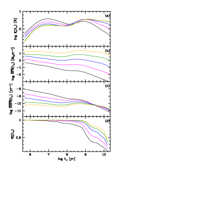
Figure 9: As Fig 8, but binning SF galaxies by their stellar mass, using five 1 dex wide bins, centered at (from bottom to top in panel b) $\log M_{\star}/M_{\odot}=7.5$, 8.5, 9.5, 10.5 and 11.5, which contain 542, 4057, 26700, 47153, 3808 galaxies, respectively.

Results grouping galaxies according to $\Sigma_{\star}$ are presented in Fig 10. Since $\Sigma_{\star}$ and $M_{\star}$ correlate very strongly ($R_{S}=0.73$ in our sample), the results are similar to those obtained grouping galaxies by their stellar mass. Kauffmann et al. (2003b), based on an analysis of two SFH-sensitive spectroscopic indices (namely $D_{n}(4000)$ and H$\delta_{A}$), propose that $\Sigma_{\star}$ is more directly connected to SFHs than $M_{\star}$. This is not obviously so comparing Figs 9 and 10. A more detailed, multivariate analysis is needed to evaluate which is the primary driver of SFHs.

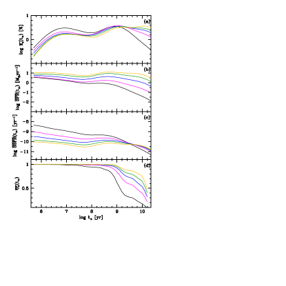
Figure 10: As Fig 8, but binning SF galaxies by their stellar surface densities, with five 0.5 dex wide bins centered at $\log\Sigma_{\star}=7.25$, 7.75, 8.25, 8.75 and 9.25 $M_{\odot}\,$kpc^-2, containing 1477, 12554, 37177, 27742, 3046 galaxies respectively.

7 Selection effects and modelling caveats

This section deals with the effects of sample selection, synthesis ingredients and model assumptions on our results.

7.1 Selection effects

We now study to which extent the mean SFHs derived in the last section are affected by the way we have defined SF galaxies. We address this issue recomputing mean SFHs for samples constructed with alternative selection criteria, and comparing to the results obtained with our default sample.

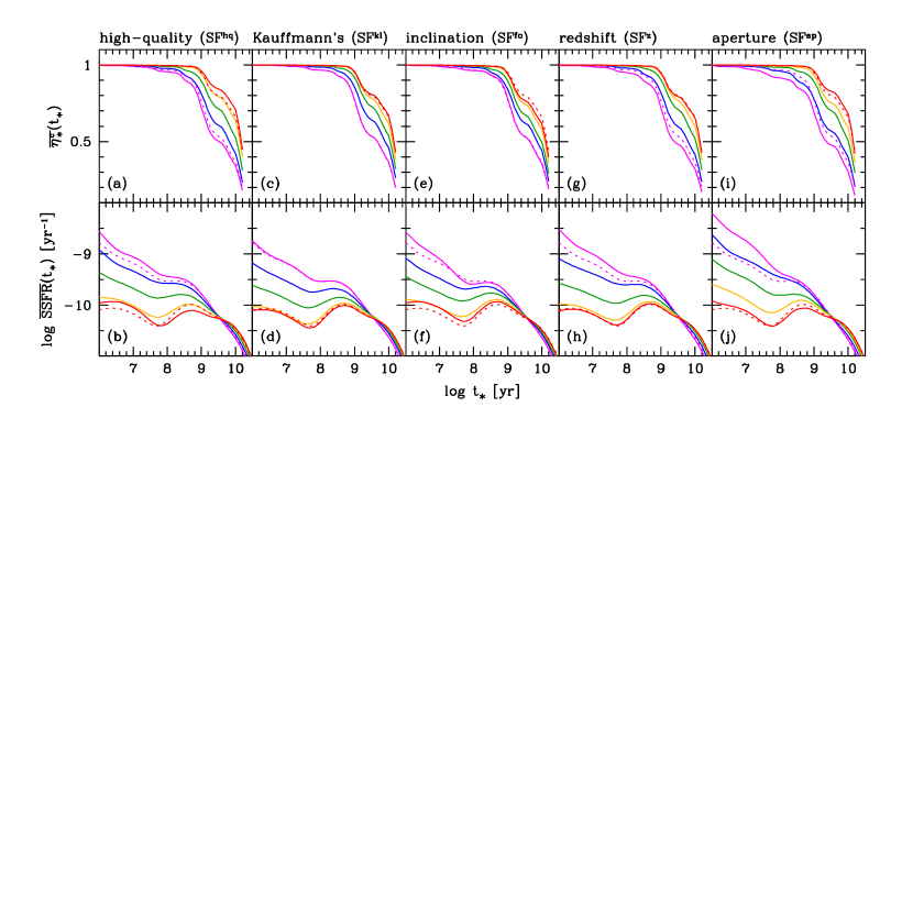
Figure 11: Average mass assembly histories ($\eta^{c}_{\star}$, top panels) and specific star formation rate (${\rm SSFR}$, bottom) histories for $Z_{neb}$-bins B to F, color-coded as in Fig 2. Solid lines show the curves for different sample definitions. For comparison, the dotted lines in all panels show the curves for bins B (lower curves; magenta) and F (upper curves; red) of the full SF sample.

We first ask how our emission line and continuum $S/N$ cuts influence our results. Figs 11a and b show the average mass assembly and SSFR functions for the high-quality SF^hq sub-sample defined in Section 2.3. The results for this better-data sub-sample are very similar to those obtained with the full SF sample. The SSFR curves in recent times are skewed to slightly higher rates, which reflects the fact that objects in the SF^hq sample are slightly younger than those in the full SF sample, as shown in Fig 3.

Our BPT-based selection of SF galaxies used the dividing line proposed in SEAGal III, which is more restrictive than the empirical line proposed by Kauffmann et al. (2003c). We define the SF^kl sample as the 111026 galaxies classified as SF according to the Kauffmann et al. (2003c) line. Fig. 11c and d show that the SFHs for $Z_{neb}$ bins in this sample are nearly indistinguishable from those obtained with the SEAGal classification criterion.

Another concern is the inclination effect. The spectra of edge-on objects are biased by the metal poorer outer parts of the galaxies, leading to an underestimation of $Z_{neb}$. This may lead us to place a galaxy in a lower $Z_{neb}$ bin than it would if it were seen face on, possibly affecting the mean SFH in that bin. To investigate this effect we have defined a sub-sample of nearly face-on galaxies, SF^fo (6842 objects), selecting by the inclination parameter, $b/a\geq 0.9$. Figs 11e and f show that the SFHs derived with this sample are practically the same as for the full sample.

Aperture effects are a common source of concern in studies of SDSS spectra (e.g., Gómez et al., 2003; SEAGal I). To investigate how such effects impact upon our SFHs we defined two samples: the SF^z sample, which comprises 58153 SF galaxies with $z\geq 0.05$ (as opposed to 0.002 for the full SF sample), and the SF^ap sample, comprising only the 1096 objects with more than half of their $z$ band luminosity inside the fiber. Both criteria exclude proportionately more the population of low $Z_{neb}$, low $M_{\star}$ galaxies (distant galaxies of this category are not present in the SDSS, due to limiting magnitude). Accordingly, the change in SFHs is only noticeable for the lowest $Z_{neb}$ bins, as shown in Figs 11g–j. In particular, Fig 11j shows that the mean SFH for bin C in the SF^ap sample matches that of bin B in the full sample. Of all selection-induced changes discussed here, this is the largest one; yet, all it does is to shift the SFHs from one group of galaxies to the adjoining one.

To summarize, selection criteria may influence the derived mean SFHs in quantitative terms, but do not modify the relative pattern of mean SFHs of galaxies in different $Z_{neb}$ bins. The same applies to grouping galaxies according to properties other than $Z_{neb}$. The general trends in the SFH as a function of global galaxy properties obtained in this work are therefore robust against variations in the sample selection criteria.

7.2 Experiments with different models

One should also ask to which extent our results are robust against changes in the base of evolutionary synthesis models. While answering this question requires an in-depth study far beyond the scope of this paper, we believe this has a much larger impact on SFHs than selection effects.

Panter et al. (2007) reported results of MOPED experiments using spectral models from different sources (Jimenez et al., 2004; Fioc & Rocca-Volmerange, 1997; Maraston, 2005; Bruzual A. & Charlot, 1993; and BC03), all sampled at $\Delta\lambda=20$ Å. For the 767 galaxies in their randomly selected test sample, the resulting mean star-formation fractions (analogous to our $\vec{\mu}$ vector) differ by factors of a few for the youngest and oldest ages, and close to a full order of magnitude for $t_{\star}\sim 0.1$–1 Gyr. Recovering SFHs in this intermediate age range is particularly hard, as discussed by Mathis et al. (2006). Indeed, the experiments reported by Panter et al. often find a suspiciously large 1 Gyr component.

The behaviour of our starlight fits is also anomalous in this age range. This is clearly seen in the mean SFHs shown in Figs 8–10, particularly in the $\vec{x}_{s}$ representation, which shows a hump at $\sim 1$ Gyr. Interestingly, starlight experiments with a base of evolutionary synthesis models using the MILES library of Sanchez-Blazquez et al. (2006, instead of the STELIB library used in the base adopted for this and previous SEAGal studies) do not produce this hump at $\sim 1$ Gyr. In fact, the whole mean SFHs derived with this new set of models differs systematically from those shown in Figs 8–10. The mass assembly function $\eta ĉ_{\star}(t_{\star})$, for instance, rises more slowly and converges at somewhat smaller $t_{\star}$ than those obtained in this work. There are also systematic differences in stellar extinction, which comes out $\Delta A_{V}^{\star}\sim 0.4$ mag larger with the MILES models. Extensive tests with these new bases, including different prescriptions of stellar evolution as well as different spectral libraries, are underway, but these first results show that significant changes can be expected.

Reassuringly, however, these same experiments show that the pattern of SFHs as a function of $Z_{neb}$, $M_{\star}$ and $\Sigma_{\star}$ reported in this paper does not change with these new models. In any case, these initial results provide an eloquent reminder of how dependent semi-empirical SFH studies are on the ingredients used in the fits.

7.3 Experiments with differential extinction

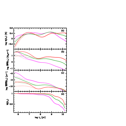
Figure 12: Comparison between mean star formation histories for the SF^hq sample modelled with only one stellar extinction (dotted lines) and with differential extinction (solid lines). For clarity, only $Z_{neb}$-bins B, D and F are drawn, and color-coding is the same as in Fig 2. Each panel shows a different representation of SFHs: (a) smoothed population vector, $\overline{x_{s}}(t_{\star})$, (b) $\overline{\rm SFR}(t_{\star})$, (c) $\overline{\rm SSFR}(t_{\star})$, and (d) $\overline{\eta^{c}_{\star}}(t_{\star})$.

We saw in Section 2.5.2 that the nebular and stellar exctintions are strongly correlated, but with $A_{V}^{neb}\sim$ twice $A_{V}^{\star}$. This indicates that the uniform stellar extinction used in our fits is not adequate to model star-forming regions, which should be subjected to a similar extinction than the line-emiting gas, ie., $A_{V}^{\star}(t_{\star}\la 10^{7}{\rm yr})\sim A_{V}^{neb}$. It is therefore fit to ask whether and how such a differential extinction affects our general results.

Given the difficulties in recovering reliable population dependent $A_{V}^{\star}$’s from spectral synthesis in the optical range alone, we address this question by postulating that populations younger than $10^{7}$ yr are extincted by $0.34+2.28A_{V}^{\star}$, i.e., the empirical $A_{V}^{neb}(A_{V}^{\star})$ relation found in Section 2.5.2, with $A_{V}^{\star}$ now denoting the extinction to $>10^{7}$ yr stars. The 17142 galaxies in the SF^hq sub-sample were re-fitted with this more realistic modified recipe for extinction effects.

Qualitatively, one expects that forcing a uniform $A_{V}^{\star}$ fit to a galaxy where the young stars suffers more extinction than the others should lead to an overestimation of the age of the young population. This older and thus redder young population would compensate the mismatch in $A_{V}^{\star}$. Allowing for $A_{V}^{\star}(t<10^{7}~{}{\rm yr})$ larger than the $A_{V}^{\star}$ of the $t>10^{7}~{}{\rm yr}$ populations makes it possible to fit the same spectrum with younger and dustier populations. Hence, the recent SFRs should increase.

This expectation is fully confirmed by these new fits. Fig. 12 shows a comparison between three $Z_{neb}$ bins (B, D and F) for the old and new fits of the SF^hq sample. One sees that the new average SFR and SSFR curves are shifted by $\sim 0.3$ dex upwards in the $t_{\star}\leq 10^{7}$ yr range with respect to the ones obtained with a single extinction. The rearrangements in the population vector tend to be in the sense of shifting some light from old populations to the $\leq 10^{7}$ yr components.

Not surprisingly, the properties which change most are those directly related to the strength of the young population, such as current SFR, which increases by 0.3 dex on average, and the mean stellar age, which decreases by $\Delta\langle\log t_{\star}\rangle_{L}\sim 0.1$ dex. The changes in other global properties such as $A_{V}^{\star}$ and $M_{\star}$ are much smaller than this.

These experiments are obviously a simplification of the problem of dust distribution in galaxies, yet they suggest that the choice of the extinction modelling can have non-negligible effects on the derived SFH curves. On the whole, however, the qualitative pattern of SFHs as a function of $Z_{neb}$ or other variables stays the same. As found in the sample selection studies, quantitative changes are at best equivalent to moving from one bin to the next, so that our general conclusion does not change.

8 Summary

In this paper we have studied physical properties of 82302 normal star-forming galaxies from the SDSS DR5, by using results from our stellar population synthesis code, starlight, and our emission-line measurement algorithm.

Before reviewing our main results, we highlight some aspects of this study which have relatively little impact upon our general conclusions, but represent significant refinements in our methodology.

1. We have detected a systematically overestimated continuum level around H$\beta$, whose origin we tentatively attribute to deficiencies in the STELIB calibration in this range. Gaussian fits to the H$\beta$ emission which disregard this offset tend to underestimate the line flux by 4% on average, and $\sim 7$% in the case of weaker lines. These are relatively small, yet systematic effects, which propagate to estimates of nebular extinction, metallicities and galaxy classification.

2. SF galaxies were selected according to the theoretical criterion proposed in SEAGal III, which minimizes contamination by AGN emission.

3. Nebular extinctions and metallicities were derived self-consistently, allowing for the metallicity dependence of the Balmer decrement. Five different reddening laws were explored, but found to produce equally good spectral fits and relatively small differences in derived physical properties.

4. We have confirmed the strong correlation between $A_{V}^{neb}$ and $A_{V}^{\star}$ found in SEAGal I. We have also identified a strong correlation between the strength of the ISM component of the NaD absorption doublet and the amount of dust derived from the synthesis.

5. Different recipes for nebular metallicity estimates were tried. Some of them proved not to be adequate for this study, either because of the lack of spectral data (e.g., measures of [ArIII]$\lambda$7135 and [OIII]4363 emission lines were available for few objects), or because such calibrations were only valid in the low-$Z_{neb}$ regime, thus encompassing a very small fraction of objects from our sample. Therefore, throughout our analysis we use the O₃N₂ index and the calibration by Stasińska (2006) to measure the nebular metallicity. Although this is not a reliable calibrator at the lowest metallicities, it is good enough for our analysis in $Z_{neb}$-bins. Furthermore, it has the nice virtue of being directly related with the position of the objects in the BPT diagram.

We now summarize results related to the main goal of this paper, namely, to investigate the SFH of galaxies along the SF wing in the BPT diagram. In practice, this means studying how SFHs change as a function of nebular metallicity, even though $Z_{neb}$ is more a product than a cause of galaxy evolution.

1. We started our study with a traditional analysis, correlating $Z_{neb}$ with several physical and observed properties. This analysis confirms results obtained directly or indirectly in the past by other works, such as relations between the nebular metallicity and galaxy luminosity, mass, dust content, mean stellar metallicity and mean stellar age.

2. Formalism towards a time-dependent analysis was then presented. Simple ways to compress the output of our stellar population synthesis code were proposed. These are based either on a posteriori smoothing of the age distribution, which allows the derivation of time dependent star formation rates, or a cumulative mass assembly history.

3. As a first application of this time dependent description of SFHs we computed the current SFR obtained from our spectral fits. The resulting values of SFR_⋆ agree very well with more traditional estimates based on the luminosity of H$\alpha$. The scatter between SFR_⋆ and SFR_Hα is just a factor of 2, despite the differences in the underlying assumptions and sensitivity to the IMF. This result strengthens confidence in our method, and, more importantly, opens the possibility of measuring current SFRs in galaxies hosting AGN, where H$\alpha$ method does not apply.

4. Fully time dependent SFHs were then derived grouping galaxies into six $Z_{neb}$ bins spanning the entire SF wing of the BPT diagram. Mean SFHs for each of these bins were presented in four different representations: (a) the smoothed population vector, $\overline{x_{s}}(t_{\star})$, (b) the star formation rates $\overline{\rm SFR}(t_{\star})$, (c) specific star formation rates $\overline{\rm SSFR}(t_{\star})$, and (d) mass-assembly histories , $\overline{\eta_{\star}^{c}}(t_{\star})$.

5. We found that SFHs vary systematically along the SF sequence. Though all galaxies assembled the bulk of their stellar mass over 1 Gyr ago, low $Z_{neb}$ systems evolve at a slower pace. Galaxies at the tip of the SF wing have current specific SFRs about 2 orders of magnitude larger than the metal rich galaxies at the the bottom of the BPT diagram.

6. At any given time, the distribution of SSFRs for galaxies within a $Z_{neb}$-bin is quite broad and approximately log-normal.

7. We performed the same SFH study grouping galaxies by their stellar mass and surface mass density. Given the existence of $Z_{neb}$–$M_{\star}$–$\Sigma_{\star}$ relations, the overall picture is obtained grouping by $Z_{neb}$. Thus, low $M_{\star}$ (low $\Sigma_{\star}$) systems are the ones which evolve slower, with current SSFRs much larger than more massive (dense) galaxies.

8. Finally, we have analysed a number of selection and modelling effects that might bias our results, and show that while they may affect the derived SFHs quantitatively, the organization of SFHs as a function of $Z_{neb}$, $M_{\star}$, $\Sigma_{\star}$ remains the same. Experiments with new evolutionary synthesis models and differential extinction fits were reported and found to lead to substantially different SFHs, yet preserving this same overall pattern.

References

- Adelman-McCarthy et al. (2007) Adelman-McCarthy et al. 2007, VizieR Online Data Catalog, 2276, 0
- Allende Prieto et al. (2001) Allende Prieto C., Lambert D. L., Asplund M., 2001, ApJ, 556, L63
- Alongi et al. (1993) Alongi M., Bertelli G., Bressan A., Chiosi C., Fagotto F., Greggio L., Nasi E., 1993, A&AS, 97, 851
- Asari (2006) Asari N. V., 2006, MSc thesis, Universidade Federal de Santa Catarina
- Baldwin et al. (1981) Baldwin J. A., Phillips M. M., Terlevich R., 1981, PASP, 93, 5
- Bica (1988) Bica E., 1988, A&A, 195, 76
- Bica et al. (1994) Bica E., Alloin D., Schmitt H. R., 1994, A&A, 283, 805
- Bica et al. (1991) Bica E., Barbuy B., Ortolani S., 1991, ApJ, 382, L15
- Bressan et al. (1993) Bressan A., Fagotto F., Bertelli G., Chiosi C., 1993, A&AS, 100, 647
- Brinchmann et al. (2004) Brinchmann J., Charlot S., White S. D. M., Tremonti C., Kauffmann G., Heckman T., Brinkmann J., 2004, MNRAS, 351, 1151
- Bruzual & Charlot (2003) Bruzual G., Charlot S., 2003, MNRAS, 344, 1000
- Bruzual A. & Charlot (1993) Bruzual A. G., Charlot S., 1993, ApJ, 405, 538
- Calzetti et al. (1994) Calzetti D., Kinney A. L., Storchi-Bergmann T., 1994, ApJ, 429, 582
- Cardelli et al. (1989) Cardelli J. A., Clayton G. C., Mathis J. S., 1989, ApJ, 345, 245
- Chabrier (2003) Chabrier G., 2003, PASP, 115, 763
- Chiappini et al. (2003) Chiappini C., Romano D., Matteucci F., 2003, MNRAS, 339, 63
- Cid Fernandes et al. (2001) Cid Fernandes R., Heckman T., Schmitt H., Delgado R. M. G., Storchi-Bergmann T., 2001, ApJ, 558, 81
- Cid Fernandes et al. (2003) Cid Fernandes R., Leão J. R. S., Lacerda R. R., 2003, MNRAS, 340, 29
- Cid Fernandes et al. (2004) Cid Fernandes R., Gu Q., Melnick J., Terlevich E., Terlevich R., Kunth D., Rodrigues Lacerda R., Joguet B., 2004, MNRAS, 355, 273
- Cid Fernandes et al. (2005) Cid Fernandes R., Mateus A., Sodré L., Stasińska G., Gomes J. M., 2005, MNRAS, 358, 363 (SEAGal I)
- Cid Fernandes et al. (2007) Cid Fernandes R., Asari N. V., Sodré L., Stasińska G., Mateus A., Torres-Papaqui J. P., Schoenell W., 2007, MNRAS, 375, L16 (SEAGal V)
- Cid Fernandes et al. (2007) Cid Fernandes et al. 2007, in preparation
- Corbin et al. (2006) Corbin M. R., Vacca W. D., Cid Fernandes R., Hibbard J. E., Somerville R. S., Windhorst R. A., 2006, ApJ, 651, 861
- Fagotto et al. (1994a) Fagotto F., Bressan A., Bertelli G., Chiosi C., 1994a, A&AS, 104, 365
- Fagotto et al. (1994b) Fagotto F., Bressan A., Bertelli G., Chiosi C., 1994b, A&AS, 105, 29
- Fioc & Rocca-Volmerange (1997) Fioc M., Rocca-Volmerange B., 1997, A&A, 326, 950
- Gallagher et al. (1984) Gallagher III J. S., Hunter D. A., Tutukov A. V., 1984, ApJ, 284, 544
- Gallazzi et al. (2005) Gallazzi A., Charlot S., Brinchmann J., White S. D. M., Tremonti C. A., 2005, MNRAS, 362, 41
- Gavazzi et al. (2002) Gavazzi G., Boselli A., Pedotti P., Gallazzi A., Carrasco L., 2002, A&A, 396, 449
- Girardi et al. (1996) Girardi L., Bressan A., Chiosi C., Bertelli G., Nasi E., 1996, A&AS, 117, 113
- Gómez et al. (2003) Gómez P. L., Nichol R. C., Miller C. J., Balogh M. L., Goto T., Zabludoff A. I., Romer A. K., Bernardi M., Sheth R., Hopkins A. M., Castander F. J., Connolly A. J., Schneider D. P., Brinkmann J., Lamb D. Q., SubbaRao M., York D. G., 2003, ApJ, 584, 210
- González-Delgado et al. (2005) González-Delgado R. M., Cerviño M., Martins L. P., Leitherer C., Hauschildt P. H., 2005, MNRAS, 357, 945
- Gordon et al. (2003) Gordon K. D., Clayton G. C., Misselt K. A., Landolt A. U., Wolff M. J., 2003, ApJ, 594, 279
- Heavens et al. (2004) Heavens A., Panter B., Jimenez R., Dunlop J., 2004, Nat, 428, 625
- Heavens et al. (2000) Heavens, A. F., Jimenez, R., & Lahav, O. 2000, MNRAS, 317, 965
- Heckman et al. (2000) Heckman T. M., Lehnert M. D., Strickland D. K., Armus L., 2000, ApJS, 129, 493
- Hopkins et al. (2003) Hopkins A. M., Miller C. J., Nichol R. C., Connolly A. J., Bernardi M., Gómez P. L., Goto T., Tremonti C. A., Brinkmann J., Ivezić Ž., Lamb D. Q., 2003, ApJ, 599, 971
- Izotov et al. (2006) Izotov Y. I., Stasińska G., Meynet G., Guseva N. G., Thuan T. X., 2006, A&A, 448, 955
- Jacoby et al. (1984) Jacoby G. H., Hunter D. A., Christian C. A., 1984, ApJS, 56, 257
- Jimenez et al. (2004) Jimenez R., MacDonald J., Dunlop J. S., Padoan P., Peacock J. A., 2004, MNRAS, 349, 240
- Kauffmann et al. (2003a) Kauffmann G. et al., 2003, MNRAS, 341, 33
- Kauffmann et al. (2003b) Kauffmann G., Heckman T. M., White S. D. M., Charlot S., Tremonti C., Peng E. W., Seibert M., Brinkmann J., Nichol R. C., SubbaRao M., York D., 2003, MNRAS, 341, 54
- Kauffmann et al. (2003c) Kauffmann G., Heckman T. M., Tremonti C., Brinchmann J., Charlot S., White S. D. M., Ridgway S. E., Brinkmann J., Fukugita M., Hall P. B., Ivezić Ž., Richards G. T., Schneider D. P., 2003, MNRAS, 346, 1055
- Kennicutt (1983) Kennicutt Jr. R. C., 1983, ApJ, 272, 54
- Kennicutt (1998) Kennicutt Jr. R. C., 1998, ApJ, 498, 541
- Kennicutt et al. (1994) Kennicutt Jr. R. C., Tamblyn P., Congdon C. E., 1994, ApJ, 435, 22
- Kong et al. (2003) Kong X., Charlot S., Weiss A., Cheng F. Z., 2003, A&A, 403, 877
- Le Borgne et al. (2003) Le Borgne J.-F., Bruzual G., Pelló R., Lançon A., Rocca-Volmerange B., Sanahuja B., Schaerer D., Soubiran C., Vílchez-Gómez R., 2003, A&A, 402, 433
- Liang et al. (2006) Liang Y. C., Yin S. Y., Hammer F., Deng L. C., Flores H., Zhang B., 2006, ApJ, 652, 257
- Maraston (2005) Maraston C., 2005, MNRAS, 362, 799
- Martins et al. (2005) Martins L. P., Delgado R. M. G., Leitherer C., Cerviño M., Hauschildt P., 2005, MNRAS, 358, 49
- Mateus et al. (2007) Mateus A., Sodré L., Cid Fernandes R., Stasińska G., 2007, MNRAS, 374, 1457 (SEAGal IV)
- Mateus et al. (2006) Mateus A., Sodré L., Cid Fernandes R., Stasińska G., Schoenell W., Gomes J. M., 2006, MNRAS, 370, 721 (SEAGal II)
- Mathis et al. (2006) Mathis H., Charlot S., Brinchmann J., 2006, MNRAS, 365, 385
- Mollá et al. (2006) Mollá M., Vílchez J. M., Gavilán M., Díaz A. I., 2006, MNRAS, 372, 1069
- Ocvirk et al. (2006) Ocvirk P., Pichon C., Lançon A., Thiébaut E., 2006, MNRAS, 365, 46
- Osterbrock & Ferland (2006) Osterbrock D. E., Ferland G. J., 2006, Astrophysics of gaseous nebulae and active galactic nuclei. Astrophysics of gaseous nebulae and active galactic nuclei, 2nd. ed. by D.E. Osterbrock and G.J. Ferland. Sausalito, CA: University Science Books, 2006
- Panter et al. (2003) Panter B., Heavens A. F., Jimenez R., 2003, MNRAS, 343, 1145
- Panter et al. (2007) Panter B., Jimenez R., Heavens A. F., Charlot S., 2007, MNRAS submitted
- Pettini & Pagel (2004) Pettini M., Pagel B. E. J., 2004, MNRAS, 348, L59
- Pilyugin & Thuan (2005) Pilyugin L. S., Thuan T. X., 2005, ApJ, 631, 231
- Raimann et al. (2000) Raimann D., Bica E., Storchi-Bergmann T., Melnick J., Schmitt H., 2000, MNRAS, 314, 295
- Reichardt et al. (2001) Reichardt C., Jimenez R., Heavens A. F., 2001, MNRAS, 327, 849
- Sanchez-Blazquez et al. (2006) Sanchez-Blazquez P., Peletier R., Jimenez-Vicente J., Cardiel N., Cenarro A. J., Falcon-Barroso J., Gorgas J., Selam S., Vazdekis A., 2006, ArXiv Astrophysics e-prints
- Sandage (1986) Sandage A., 1986, A&A, 161, 89
- Scalo (1986) Scalo J. M., 1986, Fundamentals of Cosmic Physics, 11, 1
- Schlegel et al. (1998) Schlegel D. J., Finkbeiner D. P., Davis M., 1998, ApJ, 500, 525
- Schmidt et al. (1991) Schmidt A. A., Copetti M. V. F., Alloin D., Jablonka P., 1991, MNRAS, 249, 766
- Schmidt (1959) Schmidt M., 1959, ApJ, 129, 243
- Schwartz & Martin (2004) Schwartz C. M., Martin C. L., 2004, ApJ, 610, 201
- Searle (1986) Searle L., 1986, in Norman C. A., Renzini A., Tosi M., eds, Stellar Populations Stellar Populations. pp 3–+
- Searle et al. (1973) Searle L., Sargent W. L. W., Bagnuolo W. G., 1973, ApJ, 179, 427
- Skillman et al. (2003) Skillman E. D., Côté S., Miller B. W., 2003, AJ, 125, 610
- Stasińska (2006) Stasińska G., 2006, A&A, 454, L127
- Stasińska et al. (2006) Stasińska G., Cid Fernandes R., Mateus A., Sodré L., Asari N. V., 2006, MNRAS, 371, 972 (SEAGal III)
- Stasińska et al. (2004) Stasińska G., Mateus Jr. A., Sodré Jr. L., Szczerba R., 2004, A&A, 420, 475
- Thomas et al. (2005) Thomas D., Maraston C., Bender R., Mendes de Oliveira C., 2005, ApJ, 621, 673
- Tinsley (1980) Tinsley B. M., 1980, Fundamentals of Cosmic Physics, 5, 287
- Tojeiro et al. (2007) Tojeiro R., Heavens A. F., Jimenez R., Panter B., 2007, MNRAS submitted, 704
- Torres-Papaqui et al. (2007) Torres-Papaqui et al. 2007, in preparation
- Tremonti et al. (2004) Tremonti C. A., Heckman T. M., Kauffmann G., Brinchmann J., Charlot S., White S. D. M., Seibert M., Peng E. W., Schlegel D. J., Uomoto A., Fukugita M., Brinkmann J., 2004, ApJ, 613, 898
- Vazdekis & Peletier (2007) Vazdekis A., Peletier R. F., eds, 2007, Stellar Populations as Building Blocks of Galaxies, IAU Symposium Proceedings of the International Astronomical Union 241 Vol. 241 of IAU Symposium
- Westera et al. (2004) Westera P., Cuisinier F., Telles E., Kehrig C., 2004, A&A, 423, 133
- Witt et al. (1992) Witt A. N., Thronson Jr. H. A., Capuano Jr. J. M., 1992, ApJ, 393, 611
- Yin et al. (2007) Yin S. Y., Liang Y. C., Hammer F., Brinchmann J., Zhang B., Deng L. C., Flores H., 2007, A&A, 462, 535
- York et al. (2000) York D. G. et al., 2000, AJ, 120, 1579