Spin Hall Effect and Spin Orbit coupling in Ballistic Nanojunctions

Abstract

We propose a new scheme of spin filtering based on nanometric crossjunctions in the presence of Spin Orbit interaction, employing ballistic nanojunctions patterned in a two-dimensional electron gas. We demonstrate that the flow of a longitudinal unpolarized current through a ballistic X junction patterned in a two-dimensional electron gas with Spin Orbit coupling (SOC) induces a spin accumulation which has opposite signs for the two lateral probes. This spin accumulation, corresponding to a transverse pure spin current flowing in the junction, is the main observable signature of the spin Hall effect in such nanostructures.

We benchmark the effects of two different kinds of Spin Orbit interactions. The first one ($\alpha$-SOC) is due to the interface electric field that confines electrons to a two-dimensional layer, whereas the second one ($\beta$-SOC) corresponds to the interaction generated by a lateral confining potential.

Introduction. The classical Hall effect occurs when an electric current flows through a conductor subjected to a perpendicular magnetic field. In this case the Lorentz force deflects the electrons, and charge builds up on one side of the conductor, resulting in an observable Hall voltageHall .

In the absence of an external magnetic field, some unconventional Hall-type effects involving the electron spin become possible in systems with Spin Orbit (SO) interactions, such as the spin Hall effect (SHE), predicted by theorists over 30 years ago[3] ; Hir . In analogy with the conventional Hall effect, an external electric field can be expected to induce a pure transverse spin current, in the absence of applied magnetic fields.

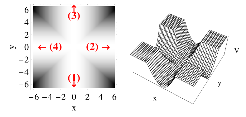
Figure 1: Density and 3D Plots of the potential $V_{c}(x,y)$ which describes the nanojunction. The junctions, in analogy with the devices proposed in ref.[Nprl, ], can be assumed as crossing junctions between two Q1D wires of width $W$ ranging between $\sim 25$ nm and $100$ nm.

In fact, the opposite spins can be separated and then accumulated on the lateral edges (probes 2 and 4 of Fig.(1)), when they are transported by a pure spin Hall current flowing in the transverse direction, in response to an unpolarized charge current in the longitudinal direction (injected in probe 1 of Fig.(1)).

When the scattering due to the impurities is spin-dependent, spin-up and spin-down electrons of an unpolarized beam are scattered into opposite directions, resulting in spin-up and spin-down charge Hall currents. The presence of the accumulation of spins shows that the SHE exists, but in this case it is extrinsic because it originates from spin-dependent scattering[3] . It was realized long ago that the extrinsic spin Hall current is the sum of two contributionsNoziéres and Lewiner (1973). The first contribution (commonly known as “skew-scattering” mechanism Smit (1955, 1958)) arises from the asymmetry of the electron-impurity scattering in the presence of spin-orbit interactions Mott and Massey (1964), the second one, i.e. the so-called “side-jump” mechanism Berger (1970, 1972); Lyo and Holstein (1972); Noziéres and Lewiner (1973), is caused by the anomalous relationship between the physical and the canonical position operatorvignale .

More recently, it has been pointed out that there may exist a different, purely intrinsic SHE. Recent theoretical arguments have unearthed the possibility for pure transverse spin Hall current, that is several orders of magnitude larger than in the case of the extrinsic effect, arising due to intrinsic mechanisms, related to the spin-split band structure in SO coupled bulk [6] ; [7] or mesoscopic 68 semiconductor systems. Often the spin currents are not directly observable, and so their detection requires measuring the spin accumulation deposited by the spin currents at the sample edges29 .

Thus, the SO coupling plays a central role in the SHE phenomenology and its properties were largely investigated in two-dimensional electron systems. Analogously to the case of the Hall effect, the SHE is based on a velocity dependent force, such as the one given by the SO interaction due to the presence of an external electric field, which, unlike the magnetic field, does not break the time reversal symmetry. The SO Hamiltonian due to an electric field, ${\bf E}({\bf r})$, is given by Thankappan

$$\hat{H}_{SO}=-\frac{\lambda_{0}^{2}}{\hbar}\;m_{0}e{\bf E}({\bf r})\cdot\left[\hat{{\bf\sigma}}\times\hat{\bf p}\right].$$ (1)

Here $m_{0}$ is the electron mass in vacuum, $\hat{{\sigma}}$ are the Pauli matrices, $\hat{\bf p}$ is the canonical momentum operator ${\bf r}$ is a 3D position vector and $\lambda_{0}^{2}=\hbar^{2}/(2m_{0}c)^{2}$.

In the present work we consider low dimensional electron systems formed by quasi-one-dimensional (Q1D) devices patterned in 2DEGs entrapped in a potential well at the interface of a heterostructure. Thus, $m_{0}$ and $\lambda_{0}$ are substituted by the effective values $m^{*}$ and $\lambda$ they take in the material. In 2DEGs there are different types of SO interactionmorozb , such as the Dresselhaus term which originates from the inversion asymmetry of the zinc-blende structure3t , the Rashba ($\alpha$-coupling) term due to the quantum-well potential Kelly ; Rashba ; Bychkov that confines electrons in the 2DEG, and the confining ($\beta$-coupling) term arising from the in-plane electric potential that is applied to squeeze the 2DEG into a quasi-one-dimensional channel Thornton ; Kelly .

A useful way to describe the effect of the SOC is to use an effective magnetic field, coplanar to the motion plane and orthogonal to the electrons speed for the $\alpha$ term, and perpendicular to the motion plane for the $\beta$ term.

In finite-size systems with SO couplings, there is always the possibility that spin Hall phenomenology (accumulation of opposite sign on the lateral edges of 2-terminal devices, or transverse spin currents in 4-terminal devices) is generated by some kind of edge effect. For the Rashba SO coupled systems this has been discussed recently in ref.ref1 , where spin-charge coupled transport was studied in disordered systems. It follows that the spin accumulation generally depends on the nature of the boundary and therefore the SHE in a SO coupled system can be viewed as a non-universal edge phenomenon. Analogously, the spin polarization induced by a current flow in a 2DEG was assumed as a geometric effect originating from special properties of the electron scattering at the edges of the sampleref2 . Moreover, in some recent papersnoish ; qse ; hatt it has been argued that the confining potential induced SO coupling will generate spin Hall like phenomenology, and it was suggested that the $\beta$ coupling yields stronger effects.

In order to discuss the different effects of the two SO terms, we formulate a Büttiker-Landauer approachBL to the spin accumulation problem in a four terminal ballistic nanojunction, by studying the electron transport at quantum wire (QW) junctions in the strongly coupled regimekirc .

The four-probe cross junction system appears to be like an ultra-sensitive scale, capable of reacting to the smallest variations of the externalkirc or effective magnetic fieldnoiq ; Nprb . In fact, any breakdown of the symmetry (left right $12-14$ in Fig.(1)) produces a transverse current (charge Hall current for the external magnetic field and pure spin current for the effective field due to the SOC). Since the effective fields due to the SOC are usually small, such devices can be quite useful, in order to obtain a spin polarized current, and have been extensively studied in recent yearsNprl ; noiq ; Nprb ; Nprin .

SO interaction in quasi-one-dimensional systems - The ballistic one-dimensional wire is a nanometric solid-state device in which the transverse motion (along $x$) is quantized into discrete modes, and the longitudinal motion ($y$ direction) is free. In this case, electrons propagate freely down to a clean narrow pipe and electronic transport with no scattering can occur.

In line with the refs.3840 , the lateral confining potential of a QW,$V_{c}(x)$, is approximated by a parabola

$$\hat{H}_{0}=\frac{{\bf p}^{2}}{2m^{*}}+V_{c}({\bf r})=\frac{{\bf p}^{2}}{2m^{*}}+\frac{m^{*}}{2}\omega^{2}x^{2}.$$ (2)

The quantity $\omega$ controls the strength (curvature) of the confining potential while the in-plane electric field $e{\bf E}_{c}({\bf r})=-\nabla V_{c}({\bf r})=-m^{*}\omega^{2}{x}$ is directed along the transverse direction.

We assume that the SO interaction Hamiltonian $\hat{H}_{SO}$ in eq. (1) is formed by two contributions $\hat{H}_{SO}=\hat{H}_{SO}^{\alpha}+\hat{H}_{SO}^{\beta}$. The first one,

$$\hat{H}_{SO}^{\alpha}=\frac{\alpha}{\hbar}\left(\hat{{\sigma}}\times\hat{\bf p}\right)_{z}=i\alpha\left(\sigma_{y}\frac{\partial}{\partial x}-\sigma_{x}\frac{\partial}{\partial y}\right),$$ (3)

arises from the interface-induced (Rashba) electric field that can be reasonably assumed to be uniform and directed along the $z$-axis. The SO-coupling constant $\alpha$ takes values within the range $\sim 10^{-11}-10^{-12}$ eV m, for different systems Das ; Nitta ; Luo ; Bychkov ; Hassenkam .

The second contribution $\hat{H}_{SO}^{\beta}$ to $\hat{H}_{SO}$ comes from the parabolic confining potential

$$\hat{H}_{SO}^{\beta}=\frac{\beta}{\hbar}\frac{x}{l_{\omega}}\left(\hat{{\sigma}}\times\hat{\bf p}\right)_{x}=i\beta\frac{x}{l_{\omega}}\sigma_{z}\frac{\partial}{\partial y}.$$ (4)

Here $l_{\omega}=(\hbar/m^{*}\omega)^{1/2}$ is the typical spatial scale associated with the potential $V_{c}$ and $\beta\equiv\lambda^{2}{m^{*}}\omega^{2}l_{\omega}$. A comparison of typical electric fields originated from the quantum-well and lateral confining potentials allows one to conclude that a plausible estimate for $\beta$ should be roughly $\sim 0.1\alpha$[morozb, ] (in a InGaAs based heterostructure with QWs of width $\sim 100nm$). Moreover, in square quantum wells where the value of $\alpha$ is considerably diminished Hassenkam ; Chen (by one order of magnitude) the constant $\beta$ may well compete in size with $\alpha$.

Eigenfunctions in a QW with $\alpha$ interaction - As we know from ref.me , the QW Hamiltonian in the presence of $\alpha$-SOC cannot be exactly diagonalized. We can calculate its spectrum (and related wavefunctions) by a numerical calculation or with simple perturbation theory. In order to get to our result, we analyze the Hamiltonian eq.(3) in the general case and separate the commuting part ($[\hat{H}_{c},\hat{H}_{0}]=0$),

$$\hat{H}_{c}=\frac{\alpha}{\hbar}p_{y}\hat{\sigma}_{x}=\frac{p_{R}p_{y}}{m^{*}}\hat{\sigma}_{x},$$ (5)

where $p_{R}=\hbar k_{R}\equiv\frac{m^{*}\alpha}{\hbar}$. The non diagonal term,

$$\hat{H}_{n}=\frac{\alpha}{\hbar}p_{x}\hat{\sigma}_{y}=\frac{\hbar p_{R}}{m^{*}l_{\omega}}(\hat{a}_{x}-\hat{a}^{\dagger}_{x})(\hat{\sigma}^{x}_{+}+\hat{\sigma}^{x}_{-}),$$ (6)

where $\hat{a}_{x},\hat{a}^{\dagger}_{x}$ are the creation-annihilation operators of the 1D quantum mechanical harmonic oscillatormess , can be neglected in the first order approximation and becomes relevant just near the crossing points $\pm k_{c}$notakc , as it was discussed in refs.[me, ; governale, ] and bibliography therein.

It follows that the Rashba subbands splitting in the energies, in the first order approximation, read

$$\varepsilon_{n,k,s_{x}}=\hbar\omega(n+\frac{1}{2})+\frac{\hbar^{2}}{2m^{*}}((k\pm k_{R})^{2}-k_{R}^{2}).$$ (7)

Here $s_{x}=+1$($-1$) corresponds to $\chi_{\rightarrow}$ ($\chi_{\leftarrow}$) spin eigenfunctions along the $x$ direction. Hence we can conclude that 4-split channels are present for a fixed Fermi energy, $\varepsilon_{F}$, corresponding to $\pm p_{y}$ and $s_{x}=\pm 1$ with eigenfunctions

$$\varphi_{\varepsilon_{F},n,s_{x}}=u_{n}(x)e^{iky}\chi_{s_{x}},$$

where $u_{n}(x)$ are displaced harmonic oscillator eigenfunctions.

Eigenfunctions in a QW with $\beta$ interaction - As it was discussed in the case of a QW, the effect of the $\beta$-SOC is analogous to the one of a uniform effective magnetic field,

$${B}_{eff}=\frac{\lambda^{2}}{\hbar}\;\frac{{m^{*}}^{2}\omega^{2}c}{e}\equiv\frac{\beta}{\hbar l_{\omega}}\frac{m^{*}c}{e},$$ (8)

orthogonal to the 2DEG directed upward or downward, according to the spin polarization along the $z$ direction.

Next we introduce $\omega_{\text{eff}}=\frac{\beta}{\hbar l_{\omega}}$, $\omega_{0}^{2}=\omega^{2}-\omega_{\text{eff}}^{2}$ and the total frequency $\omega_{T}=\sqrt{\omega^{2}+\omega_{\text{eff}}^{2}}$, thus

$$\hat{H}_{0}+\hat{H}^{\beta}_{SO}=\frac{\omega_{0}^{2}}{\omega_{T}^{2}}\frac{p_{y}^{2}}{2m^{*}}+\frac{p_{x}^{2}}{2m^{*}}+\frac{m^{*}\omega_{T}^{2}}{2}(x-x_{0})^{2},$$ (9)

where $x_{0}=s\frac{\omega_{c}\omega_{\text{eff}}p_{y}}{\omega_{T}^{2}m^{*}}$, $s=\pm 1$, corresponds to the spin polarization along the $z$ direction. 4 spin channels are present for a fixed Fermi energy $\varepsilon_{F}$, corresponding to $\pm p_{y}$ and $s_{z}=\pm 1$ with wavefunctions

$$\varphi_{\beta,\varepsilon_{F},n,s_{z}}(x,y)=u_{n}(x+s_{z}x_{0})e^{iky}\chi_{s_{z}}.$$

The junction - Starting from the model of a QW, we are able to write the model potential energy of the electrons in the x-y plane as $V_{c}(x,y)=\frac{m^{*}\omega^{2}}{2}x^{2}$ for $|y|>|x|$ and $V_{c}(x,y)=\frac{m^{*}\omega^{2}}{2}y^{2}$ for $|x|>|y|$, for QWs running along the x and y axes as in Fig.(1) (see ref.[kirc, ]).

Next we follow the quantum mechanical approach to the calculation of electron scattering proposed by Kirczenow in ref.[kirc, ]. This approach is based on the analytic solution of the quantum-mechanical Schrödinger equation in each of the four QWs.

$\alpha$-Coupling - In each of the four QWs, $H^{\alpha}$ has eigenfunctions belonging to 1D subband ($n=0,1,...$) given by

$$f^{\parallel}_{n,q,\rightarrow}=u_{n}(x)e^{iqy}e^{ik_{R}y}\chi^{x}_{\rightarrow}\quad f^{\parallel}_{n,q,\leftarrow}=u_{n}(x)e^{iqy}e^{-ik_{R}y}\chi^{x}_{\leftarrow},$$

$$f^{=}_{n,q,\rightarrow}=u_{n}(y)e^{iqx}e^{ik_{R}x}\chi^{y}_{\rightarrow}\quad f^{=}_{n,q,\leftarrow}=u_{n}(y)e^{iqx}e^{-ik_{R}x}\chi^{y}_{\leftarrow},$$

where $\parallel$ stands for wire 1 or 3 and $=$ for wire 2 or 4. An electron in subband $n$ having spin $s_{x}=s$ and wavevector

$$k_{w}^{s}(\varepsilon_{F},n)=sk_{R}\pm\sqrt{k_{R}^{2}+k_{n}^{2}}\equiv sk_{R}\pm q,$$

where $k_{n}^{2}=2m^{*}\left(\varepsilon_{F}-\hbar\omega_{T}(n+\frac{1}{2})\right)$ and $q=\sqrt{k_{R}^{2}+k_{n}^{2}}$, is incident on the junction from wire 1. The electron eigenstate is given by $\psi=\psi^{i}$ in wire $i=1,2,3,4$ respectively, where $\psi^{1}=f^{1}_{n,k,s}+\sum_{r,s^{\prime}}a^{1}_{r,s^{\prime}}f^{1}_{r,-k,s^{\prime}}$ and $\psi^{j}=\sum_{r}a^{j}_{r,s^{\prime}}f^{j}_{r,\pm k,s^{\prime}}$ for $j=2,3,4$ ($+$ for $j=2$ and $3$, $-$ for $j=4$). The sums are over all subbands, including those with imaginary $q$ (evanescent partial waves). The expansion coefficients $a^{i}_{r,s^{\prime}}$, and the scattering probabilities $T_{i,j}^{s,s^{\prime}}$, were found numerically from the continuity of $\psi$ and $\nabla\psi$ at $x=\pm y$.

If we limit ourselves to the lowest subband ($n=0$), the out of plane $\langle S_{z}({\bf r})\rangle$ component of the spin accumulation (local spin density) can be obtained in each probe as a simple function of the expansion coefficients:

$$\langle S^{i}_{z}(\xi,\eta)\rangle=\frac{\hbar}{2}S^{i}_{0}\cos(2k_{R}\eta+\delta_{i}).$$ (10)

Here $S^{i}_{0}=|a^{i}_{0,\rightarrow}(a^{i}_{0,\leftarrow})^{*}|$, $\delta_{i}=Arg\left(a^{i}_{0,\rightarrow}(a^{i}_{0,\leftarrow})^{*}\right)$ while $(\xi,\eta)$ are $(y,x)$ in probe 2, $(x,y)$ in probe 3 and $(y,-x)$ in probe 4. From eq.(10) we obtain the known spin oscillations, upon which the Datta-Das device for the spin filtering is also basedme . These oscillations can disappear in a device like the one proposed in ref.Nprl , where the SO interaction vanishes out of the crossing zone. When a spin unpolarized current is injected in lead 1, it yields $S^{2}_{0}=S^{4}_{0}$ and $S^{3}_{0}=0$, as a consequence of the symmetry of the system.

Next let us turn to considering the presence of opposite spin polarizations in the two opposite probes 2 and 4 of the nanojunction. The phase difference $\delta_{2}-\delta_{4}$ is responsible for a net spin polarization of the current transmitted in the two transverse leads. If we introduce two collectors at a distance $L_{c}<\frac{\pi}{4k_{R}}$ from the center of the junction, no oscillations are present.

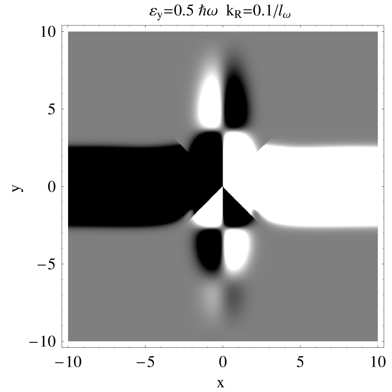
Figure 2: The out-of-plane component $\langle S_{z}({\bf r})\rangle$ of the spin accumulation induced by the quantum transport of the unpolarized charge current injected from the lead 1 into a 4-terminal cross junction ($k_{R}l_{\omega}=0.1$). This picture shows how lateral spin-$\uparrow$ (white) and spin-$\downarrow$ (black) densities flow in opposite directions through the transverse leads to generate a linear response spin Hall current $I_{sH}$, which changes sign upon reversing the bias voltage (i.e. injecting the current in lead 4). Here we display only the current exiting from the junction, thus we observe unpolarized currents in leads 1 and 3. Since the local spin density is due to the evanescent states, it is negligeable everywhere, except in proximity of the center of the junction.

Thus, as shown in Fig.(2), obtained taking into account the first 5 subbands, lateral spin-$\uparrow$ and spin-$\downarrow$ densities will flow in opposite directions through the transverse leads. This behaviour is unchanged if we substitute the collectors by ideal leads with vanishing SO interaction.

For evaluating the order of magnitude corresponding to the spin polarization, we can calculate the dependence of $S_{z}$ on the strength of the Rashba coupling.

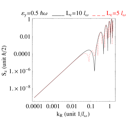
Figure 3: The dependence of the maximum value of the out-of-plane component of the spin accumulation on the strength of the SO coupling (reported in logarithmic scale). On the left we display the case of $\alpha$-SOC where $S_{z}$ is reported as a function of $k_{R}$. On the right we show the case of $\beta$-SOC where the coupling is expressed in terms of $\omega_{\text{eff}}$ in units of ($\omega$). Notice that the abscissa of the two graphs is the same, in fact $k_{R}l_{\omega}=\frac{\alpha}{l_{\omega}\hbar\omega}$ while $\frac{\omega_{eff}}{\omega}=\frac{\beta}{l_{\omega}\hbar\omega}$.

In the left panel of Fig.(3) we show the spin polarization, as a function of the Rashba wavevector $k_{R}$, for two different values of the distance between the collectors and the center of the junction, i.e. $L_{c}=5l_{\omega}$ and $L_{c}=10l_{\omega}$.

Next we discuss some realistic or theoretical devices, capable of acting as spin filters based on the Rashba interaction. In usual devicesmorozb , the natural value reads $\alpha_{0}\sim 10^{-11}eV\,m$ and we obtain $k_{R}\sim 10^{-4}nm^{-1}$, whereas a typical nanojunction should be made by using narrow QWs of a width, W, from $25$ to $75nm$, corresponding to $l_{\omega}\sim 5$ to $15nm$. It follows that $k_{R}l_{\omega}$ ranges between $10^{-3}$ and $10^{-2}$, corresponding to a spin value $\langle S_{z}\rangle$ between $10^{-7}$ and $10^{-5}$ $\hbar/2$, as we show in Fig.(3).

In the device proposed in ref.[Nprl, ] the value of $\alpha$ can take values up to $\sim 6\times 10^{2}\alpha_{0}$, while $W$ is $\sim 25nm$, and we have the value $k_{R}l_{\omega}\lesssim 0.3$, corresponding to a spin value $\langle S_{z}\rangle$ which ranges from $10^{-4}$ to $10^{-3}$ $\hbar/2$, in agreement with the results reported there.

$\beta$-Coupling - In each of the four QWs $H^{\beta}$ has eigenfunctions belonging to a 1D subband ($n=0,1,...$) given by

$$f^{\parallel}_{n,q,s}=u_{n}(x-sx_{0})e^{iky}\chi^{z}_{\uparrow}$$

$$f^{=}_{n,q,s}=u_{n}(y-sx_{0})e^{ikx}\chi^{z}_{\downarrow}.$$

An electron in subband $n$, having spin $s_{z}=s$ and wavevector $k(\varepsilon_{F},n)$, is incident on the junction from wire 1. We can evaluate the transmission coefficient from the expansion coefficients as we did above, whereas in this case no oscillations will be observed in the spin polarization ($[H^{\beta},S_{z}]=0$).

Here we limit ourselves to the lowest subband ($n=0$), thus the out of plane $\langle S_{z}({\bf r})\rangle$ component of the spin accumulation can be easily obtained in each probe and does not depend on the distance of the collectors.

Also in this case we discuss some devices able to act as spin filters, here based on the $\beta$-SOC. We carry out a comparison with the results recently reported in ref.[hatt, ] (the fundamental parameter in that paper is $\alpha$, corresponding to $\lambda^{2}$ in this article, while the ratio $\alpha/l^{2}$ corresponds to $\lambda^{2}/l_{\omega}^{2}=\omega_{\text{eff}}/\omega$).

In ref.[hatt, ] the variation of $G_{sH}$ was discussed with the SO coupling strength for $0<\omega_{\text{eff}}/\omega<1$. The authors showed that $G_{sH}$ increases with $\omega_{\text{eff}}$, up to the value $\sim 0.2\omega$, and then it tends to saturate. This prediction is in agreement with the predicted spin polarization in the transverse leads that saturates between $0.1<\omega_{\text{eff}}<1$, as shown in the right panel of Fig.(3). Moreover, we predict some oscillations near $\omega_{\text{eff}}\sim 0.1\omega$, corresponding to the quenching oscillations discussed in ref.[noiq, ]

The SOC strengths have been theoretically evaluated for some semiconductors compounds[41, ]. In a QW patterned in InGaAs/InP heterostructures, $\lambda^{2}$ takes values between $50$ and $150\,{\AA}^{2}$, hence ($\beta\sim 0.1\alpha_{0}$morozb ). Thus, one has $\hbar\omega_{\text{eff}}\sim 10^{-6}-10^{-4}eV$, corresponding to $\omega_{\text{eff}}/\omega\sim 10^{-4}-10^{-3}$. For GaAs heterostructures, $\lambda^{2}$ is one order of magnitude smaller ($\sim 4.4{\AA}^{2}$) than in InGaAs/InP, whereas for HgTe based heterostructures it can be more than three times largerHgTe . However, the lithographical width of a wire defined in a 2DEG can be as small as $20nm$kunze ; thus we can realistically assume that $\omega_{\text{eff}}/\omega$ runs from $1\times 10^{-6}$ to $1\times 10^{-1}$ (always away from the saturation region).

In any case $W$ should be larger than $\lambda_{F}$, so that at least one conduction mode is occupied. In this realistic range of values the spin polarization due to the $\beta$-SOC turns out to be at least one order of magnitude larger than the one due to the corresponding value of the $\alpha$-SOC assumed as $\alpha\sim 10\beta$. Thus we can conclude that, for devices patterned in a 2DEG at a nanometric scale, the $\beta$ coupling has stronger effects than the $\alpha$ coupling, as it can be seen by comparing the two panels of Fig.(3).

Conclusions - In this paper we propose a new scheme of spin filtering based on nanometric crossjunctions in the presence of SO interaction. The cross geometry seems to be one of the most efficient devices for the spin filtering, because it acts like an ultra-sensitive scale, capable of reacting to the smallest variations of both external and effective fields. Here we discussed the SHE in such a small ballistic device, in which the SOC arises due to the in-plane confining potential ($\beta$), in contrast to the more widely studied situation of the Rashba SOC ($\alpha$).

Our approach allows us to make a comparison between the effects due to each term of SOC, thus we demonstrate that in many cases the spin filtering based on $\beta$-SOC can be more efficient than the one based on the $\alpha$-SOC. It happens in nanometric crossjunction with opportune values of $\lambda$, thus the feasibility of similar devices depends on their size and on the materials.

We acknowledge the support of the grant 2006 PRIN ”Sistemi Quantistici Macroscopici-Aspetti Fondamentali ed Applicazioni di strutture Josephson Non Convenzionali”.

References

- (1) The Hall Effect and its Applications, edited by C. L. Chien and C.W. Westgate (Plenum, New York, 1980).
- (2) M. I. D’yakonov and V. I. Perel’, JETP Lett. 13, 467 (1971).
- (3) J. E. Hirsch, Phys. Rev. Lett. 83, 1834 (1999)
- (4) B. K. Nikolic, S. Souma, L. P. Zarbo, and J. Sinova Phys. Rev. Lett. 95, 046601 (2005).
- Noziéres and Lewiner (1973) P. Noziéres and C. Lewiner, J. Phys. (Paris) 34, 901 (1973).
- Smit (1955) J. Smit, Physica 21, 877 (1955).
- Smit (1958) J. Smit, Physica 24, 39 (1958).
- Mott and Massey (1964) N. F. Mott and H. S. W. Massey, The Theory of Atomic Collisions (Oxford University Press, 1964).
- Berger (1970) L. Berger, Phys. Rev. B 2, 4559 (1970).
- Berger (1972) L. Berger, Phys. Rev. B 5, 1862 (1972).
- Lyo and Holstein (1972) S. K. Lyo and T. Holstein, Phys. Rev. Lett. 29, 423 (1972).
- (12) E. M. Hankiewicz and G. Vignale,Coulomb corrections to the extrinsic spin-Hall effect of a two-dimensional electron gas cond-mat0507228
- (13) S. Murakami, N. Nagaosa, and S. C. Zhang, Science 301, 1348 (2003).
- (14) J. Sinova, D. Culcer, Q. Niu, N. A. Sinitsyn, T. Jungwirth, and A. H. MacDonald, Phys. Rev. Lett. 92, 126603 (2004).
- (15) L. Sheng, D. N. Sheng, and C. S. Ting, Phys. Rev. Lett. 94, 016602 (2005); E. M. Hankiewicz, L.W. Molenkamp, T. Jungwirth, J. Sinova, Phys. Rev. B 70, 241301(R) (2004).
- (16) Y. K. Kato, R. C. Myers, A. C. Gossard, and D. D. Awschalom, Science 306, 1910 (2004); J. Wunderlich, B. Kaestner, J. Sinova, and T. Jungwirth, Phys. Rev. Lett. 94, 047204 (2005).
- (17) L. D. Landau, E. M. Lifshitz, Quantum Mechanics (Pergamon Press, Oxford, 1991).
- (18) A. V. Moroz and C. H. W. Barnes, Phys. Rev. B 61, R2464 ( 2000).
- (19) G. Dresselhaus, Phys. Rev. 100, 580 (1955).
- (20) M. J. Kelly Low-dimensional semiconductors: material, physics, technology, devices (Oxford University Press, Oxford, 1995).
- (21) E. I. Rashba, Fiz. Tverd. Tela (Leningrad) 2, 1224 (1960) [Sov. Phys. – Solid State 2, 1109 (1960)].
- (22) Yu. A. Bychkov, E. I. Rashba, Pis’ma Zh. Eksp. Teor. Fiz. 39, 66 (1984) [JETP Lett. 39, 78 (1984)].
- (23) T. J. Thornton, M. Pepper, H. Ahmed, D. Andrews, and G. J. Davies, Phys. Rev. Lett. 56, 1198 (1986).
- (24) V. M. Galitski, A. A. Burkov, and S. Das Sarma, Phys. Rev. B 74, 115331 (2006)
- (25) A. Reynoso, Gonzalo Usaj, and C. A. Balseiro, Phys. Rev. B 73, 115342 (2006)
- (26) S. Bellucci and P. Onorato, Phys. Rev. B 73, 045329 (2006).
- (27) B. A. Bernevig and S. C. Zhang, Phys. Rev. Lett. 96, 106802 (2006).
- (28) K. Hattori and H. Okamoto , Phys. Rev. B 74, 155321 (2006).
- (29) M. Büttiker Phys. Rev. Lett. 57, 1761 (1986).
- (30) G. Kirczenow Phys. Rev. Lett. 62, 2993, (1989).
- (31) S. Bellucci and P. Onorato, Phys. Rev. B74, 245314 (2006).
- (32) B. K. Nikolic, L. P. Zarbo and S. Souma Phys. Rev. B 72, 075361 (2005).
- (33) S. Souma and B.K. Nikolić, Phys. Rev. Lett. 94, 106602 (2005).
- (34) S. E. Laux, D. J. Frank, and F. Stern, Surf. Sci. 196, 101 (1988); H. Drexler et al., Phys. Rev. B49, 14074 (1994); B. Kardynałet al., Phys. Rev. B55, R1966 (1997).
- (35) B. Das, S. Datta, and R. Reifenberger, Phys. Rev. B41, 8278 (1990).
- (36) J. Nitta, T. Akazaki, H. Takayanagi, and T. Enoki, Phys. Rev. Lett. 78, 1335 (1997).
- (37) J. Luo, H. Munekata, F. F. Fang, and P. J. Stiles, Phys. Rev. B41, 7685 (1990).
- (38) T. Hassenkam, S. Pedersen, K. Baklanov, A. Kristensen, C. B. Sorensen, P. E. Lindelof, F. G. Pikus, and G. E. Pikus, Phys. Rev. B55, 9298 (1997).
- (39) G. L. Chen, J. Han, T. T. Huang, S. Datta, and D. B. Janes, Phys. Rev. B47, 4084 (1993).
- (40) S. Bellucci and P. Onorato, Phys. Rev. B 68, 245322 (2003); S. Bellucci and P. Onorato, Phys. Rev. B 72, 045345 (2005).
- (41) A. Messiah, Quantum Mechanics (North-Holland, Amsterdam, 1961)
- (42) .
- (43) M. Governale, U. Zuelicke, Phys. Rev. B 66, 073311 (2002).
- (44) E. A. de Andrada e Silva, G. C. La Rocca, and F. Bassani, Phys. Rev. B 55, 16293 (1997).
- (45) X. C. Zhang, A. Pfeuffer-Jeschke, K. Ortner, V. Hock, H. Buhmann, C. R. Becker, and G. Landwehr, Phys. Rev. B 63, 245305 (2001).
- (46) M. Knop, M. Richter, R. Maßmann, U. Wieser, U. Kunze, D. Reuter, C. Riedesel, and A. D. Wieck, Semicond. Sci. Technol. 20, 814 (2005).