DEVELOPMENT OF PHYSICALLY BASED PLASTIC FLOW RULES FOR BODY-CENTERED CUBIC METALS WITH TEMPERATURE AND STRAIN RATE DEPENDENCIES

Chapter 1 Introduction

We say that we will put the sun into a box. The idea is pretty.

The problem is, we don’t know how to make the box.

Pierre-Gilles de Gennes

Refractory metals crystalizing in the body-centered cubic (bcc) structure are materials employed in many modern applications such as structural components of fusion reactors or kinetic energy penetrators. Modern nuclear applications seek materials that exihibit large radiographic densities that allow for shielding or collimation of radiation (Zinkle et al.,, 2002). This requirement disqualifies most of the usual structural materials because they yield rather bulky components. Apart from very dense alloys that are often inapplicable due to their prohibitive cost, the pool of potential candidates comprises pure forms of refractory metals and iron.

One of the fundamental requirements for every structural material is its stability under mechanical loading in a given range of working conditions. In structural applications, a material is frequently regarded to loose its functionality upon reaching the yield limit state when a permanent macroplastic deformation sets in. For a given loading, this limiting state can be predicted theoretically using a proper yield criterion that is independent of the shape of the structural component.

1.1 Historical background

The experimental studies of plastic flow of crystalline materials date back to the work of Taylor and Elam, (1925) and Taylor and Farren, (1926) on face-centered cubic (fcc) aluminum, and to Elam, (1926) on fcc copper and gold. These materials were found to deform by sliding of close-packed atomic planes, $\{111\}$, over each other in the direction of densest atomic packing, $\langle{110}\rangle$. Around the same time, similar experiments on body-centered cubic (bcc) $\alpha$-iron were carried out by Taylor and Elam, (1926). In this material, the deformation occured by crystallographic planes sliding virtually parallel to the $\langle{111}\rangle$ axis which is the direction of closest atomic packing but, unlike in fcc aluminum, copper and gold, the slip plane was not well-defined. Instead, the plane of slip appeared to be related to the distribution of stress albeit coinciding with a plane containing the $\langle{111}\rangle$ slip direction. Perhaps even more surprising was the observation that the sliding of parallel atomic planes did not occur by a rigid displacement of one plane over the other but, instead, the particles of the material appeared to “cling” together in lines or rods. Two years later, Taylor, (1928) performed similar experiments on $\beta$-brass with B2 structure whose lattice is composed of two interpenetrating simple cubic (sc) lattices of copper and zinc. For some orientations, the slip plane did not coincide with any well-defined crystallographic plane, similarly as in $\alpha$-iron, although for other orientations the slip occured on $\{110\}$ planes, as expected. Unlike $\alpha$-iron, the resistance to slipping two parallel planes over each other in $\beta$-brass depended on the sense of slip. Furthermore, the magnitudes of axial compressive stresses needed to plastically deform single crystals of $\alpha$-iron and $\beta$-brass were significantly larger than those employed in earlier experiments on fcc aluminum (Taylor and Elam,, 1925; Taylor and Farren,, 1926).

The marked differences in plastic deformation of fcc and bcc metals led Schmid and Boas, (1935) to investigate hexagonal close-packed (hcp) metals zinc and cadmium. The single crystals of these metals were observed to deform in a similar way as aluminum, copper and gold. These observations together with the earlier results of studies on the fcc metals were condensed into the so-called Schmid law according to which the macroscopic plastic deformation occurs when the shear stress parallel to the slip direction resolved in the most highly stressed slip system attains its critical value. Although the Schmid law was originally deemed to be generally valid for any crystalline material, its deficiency in bcc metals was known already from the works of Taylor and Elam, (1926) on $\alpha$-iron and of Taylor, (1928) on $\beta$-brass. This implies that the mechanism governing the plastic flow of bcc metals is likely to be different from that of fcc and hcp metals.

The observations of Taylor and Elam, (1926) remained puzzling until the birth of the concept of dislocations established by three classical papers by Orowan, (1934), Polanyi, (1934) and Taylor, (1934) that provided the needed microscopic understanding of the plastic flow of crystalline materials. Dislocations soon became recognized as carriers of plastic flow, which immediately raised important questions about their behavior under stress and later also the effect of temperature on their motion. Since the propagation of dislocations requires a collective motion of many atoms, it was impossible to obtain the atomic positions as a rigorous solution of some equilibrium conditions. Instead, the periodic structure of the crystal in the glide plane was represented by a continous function that merely obeyed the periodicity of the lattice (Peierls,, 1940). Based on this model, the shear stress to move the dislocation was predicted to be about one-thousandth of the theoretical shear strength of a perfect lattice (Nabarro,, 1947), a hundred times smaller value than the yield stresses normally encountered in experiments on bcc metals. The final breakthrough came two decades later, when Hirsch, (1960) realized that the screw dislocation core has to obey the underlying three-fold screw symmetry of the $\langle{111}\rangle$ direction in the bcc lattice and may spread into three planes in the zone of this direction. He postulated that, provided the screw dislocation core spreads on several planes that all contain the $\langle{111}\rangle$ slip direction, a high stress would be needed to transform this initially sessile core into a configuration that is glissile in a slip plane. This conjecture not only provided a plausible explanation of the origin of large Peierls stresses but also implied a strong temperature dependence and complex slip geometry in bcc metals.

1.2 Low-temperature experiments

One of the most notable characteristics of the plastic deformation of bcc metals is a steep increase of both yield and flow stresses with decreasing temperature, which had been a matter of debate for many years and attributed by some to the effect of impurities. This hypothesis survived until the discovery of new purification techniques such as electron beam floating zone method and ultra-high-vacuum annealing that provided macroscopic single crystals essentially free of interstitial solutes. Even in these high-purity bcc metals, the plastic flow at temperatures below $0.1T_{m}$, where $T_{m}$ is the melting temperature, displayed remarkable differences with respect to the behavior of close-packed metals. Among the most important ones were the tendency to cleave at low temperatures, large strain rate sensitivity, strong influence of interstitial impurities and, most remarkably, a tension-compression asymmetry detected in uniaxial loading tests of single crystals of practically all bcc metals (Christian,, 1983). This asymmetry was originally attributed to the so-called twinning-antitwinning asymmetry of shearing in the $\langle{111}\rangle$ slip direction along $\{112\}$ planes.

The majority of the early experiments have been done on niobium (Mitchell et al.,, 1963; Duesbery,, 1969; Bolton and Taylor,, 1972; Louchet and Kubin,, 1975; Reed and Arsenault,, 1976; Bowen and Taylor,, 1977), tantalum (Webb et al.,, 1974; Shields et al.,, 1975; Nawaz and Mordike,, 1975; Takeuchi and Maeda,, 1977; Wasserbäch and Novák,, 1985), molybdenum (Vesely,, 1968; Guiu,, 1969; Matsui and Kimura,, 1976; Saka et al.,, 1976; Kitajima et al.,, 1981; Matsui et al.,, 1982; Aono et al.,, 1983), and $\alpha$-iron (Allen et al.,, 1956; Arsenault,, 1964; Keh,, 1965; Aono et al.,, 1981). On the other hand, significantly less attention has been devoted to tungsten (Argon and Maloof,, 1966; Tabata et al.,, 1976; Brunner,, 2004) owing to the complicated purification process caused by its extremely high melting temperature. Similar experiments on alkali metals have long been impossible due to their strong reactivity to water and rapid oxidization in air, and have been limited so far to potassium (Basinski et al.,, 1981; Duesbery and Basinski,, 1993; Pichl and Krystian, 1997c, ) which retains its bcc structure down to the lowest temperatures investigated. On the other hand, experiments on bcc sodium and lithium are rather rare (Pichl and Krystian, 1997a, ), mainly due to their martensitic transformation to close-packed structures at low temperatures.

Pure bcc metals at low temperatures exhibit a phenomenon called anomalous slip which was first observed experimentally on single crystals of niobium (Duesbery and Foxall,, 1969; Bolton and Taylor,, 1972), and later in vanadium (Taylor et al.,, 1973), tantalum (Nawaz and Mordike,, 1975), molybdenum (Matsui and Kimura,, 1976; Kitajima et al.,, 1981) and tungsten (Kaun et al.,, 1968). In these experiments the slip did not occur on the most highly stressed slip system, as expected, but typically on the fourth or fifth most highly stressed $\{110\}\langle{111}\rangle$ system. At the same time, the slip traces of the expected slip system with the highest Schmid stress were discontinuous or sometimes not observed at all. Similar behavior was also observed in dilute transition metal alloys (Jeffcoat et al.,, 1976; Taylor and Saka,, 1991) and alkali metals (Pichl and Krystian, 1997c, ). In contrast, the low-temperature form of ferromagnetic $\alpha$-iron deforms exclusively by slip on the most highly stressed slip system (Aono et al.,, 1981) and the anomalous slip has never been observed.

The direct observation of dislocations was first performed on single crystals of gold and aluminum (Hirsch et al.,, 1956), as recalled by Hirsch, (1980) in his review of the period 1946-56. The evolution of high-resolution electron microscopy (HREM) recently allowed to observe the dislocation core structure in thin foils of bcc metals (Sigle,, 1999). However, since screw dislocations in few-nanometer thick foils, which are currently employed in the HREM studies, inherently generate the so-called Eshelby twist (Eshelby and Stroh,, 1951), the interpretation of these measurements is still a matter of controversy (Mendis et al.,, 2006).

1.3 Theoretical studies and computer simulations

The modern theoretical studies of the motion of screw dislocations in bcc metals were initiated by the study of internal friction in polycrystalline copper (Seeger,, 1956). At high temperatures and low applied stresses, screw dislocations were postulated to move by nucleating two non-screw segments, called kinks, that connected the original straight screw dislocation with its activated segment lying in the neighboring valley of the Peierls potential. This work was generalized to finite stresses by Dorn and Rajnak, (1964) by solving for the stationary shape of the dislocation in the presence of applied stress. They demonstrated that, at finite applied shear stress parallel to the slip direction, the dislocation surmounts the Peierls barrier by nucleating a critical bow-out represented by a smooth local deflection of otherwise straight dislocation line. For a prototypical Peierls potential whose shape merely obeyed the periodicity of the lattice in the slip plane, these studies correctly predicted the increasing trend of the yield stress with decreasing temperature for all refractory metals and $\alpha$-iron. The shape of the Peierls potential and its effect on the temperature dependence of the yield stress was recently studied by Suzuki et al., (1995), who concluded that the best agreement with experiment is obtained if the Peierls potential exhibits a flat maximum or a “camel-hump” shape with an intermediate minimum. However, since the Peierls potential was still defined as a one-dimensional function of the position of the dislocation in the slip plane, this model could not reproduce the cross-slip in bcc metals and the onset of anomalous slip frequently encountered in low-temperature experiments. In order to allow for these phenomena to occur, Edagawa et al., (1997) recently suggested that the Peierls potential should be a two-dimensional function of the position of the intersection of the dislocation line with the $\{111\}$ plane.

Computer-based atomistic modeling of the structure and energetics of screw dislocations using simple pair potentials became possible around 1970 and was mainly pioneered by Duesbery, (1969), Vitek et al., (1970), and Basinski et al., (1971). As envisaged already by Hirsch, (1960), the unstressed dislocation cores possessed the three-fold symmetry of the underlying lattice and extended on the three $\{110\}$ planes containing the $\langle{111}\rangle$ slip direction. Because two such configurations of the same energy were found that were related by a diad symmetry, the core has been called as degenerate. Subsequent studies of dislocations under stress revealed that the spreading of the core on the three $\{110\}$ planes is indeed responsible for a strong twinning-antitwinning asymmetry of the shear stress parallel to the slip direction (Christian,, 1983). In the following years, these simulations were revisited using more accurate potentials such as Finnis-Sinclair (F-S) or Embedded Atom Method (EAM) that a priori include also the many-body contribution to the total energy (Duesbery and Vitek,, 1998). The latter was further extended to incorporate the directional bonding that gave rise to the Modified Embedded Atom Method (MEAM) (Baskes,, 1992).

Currently the most accurate semi-empirical schemes formulated in real-space are the Modified Generalized Pseudopotential Theory (MGPT) (Moriarty,, 1988; Xu and Moriarty,, 1996, 1998) and the Bond Order Potential (BOP) (Pettifor,, 1995; Horsfield et al.,, 1996). The latter is an $O(N)$, two-center orthogonal tight binding method that correctly describes the mixed metallic and covalent character of bonding in $d$-electron transition metals. In BOP, the bonding part is obtained directly from the first-principles calculations, while the rest of the potential is constructed purely empirically to reproduce such fundamental parameters as the lattice constant, cohesive energy, and elastic moduli. The incorporation of directional bonding revealed a new structure of the dislocation core that spreads symmetrically on the three $\{110\}$ planes. This, so-called non-degenerate core possesses not only the three-fold symmetry dictated by the lattice but also an additional $[\bar{1}01]$ diad symmetry. Since the number of atoms employed in these simulations is usually of the order of thousands, they allow extensive atomistic simulations of the onset of plastic flow, the results of which can be used as a basis for the development of continuum laws of plasticity in bcc metals.

The most basic simulations of dislocations in bcc metals utilize the first-principles-based Density Functional Theory (DFT). Since this theory is formulated in k-space, it necessitates the use of periodic simulation cells whose boundary conditions must eliminate the contribution of the periodic images of the dislocation in the neighboring cells. One of the most recent achievements in the simulation of dislocations using DFT is the work of Woodward and Rao, (2001, 2002) introducing the flexible Green’s function boundary condition (GFBC) that self-consistently couples the local dislocation strain field with the long-range elastic field. This method predicts the existence of the same non-degenerate dislocation core as obtained by BOP.

Apart from the single dislocation molecular statics simulations at $0~{}{\rm K}$ outlined above that aim at studying the plasticity of bcc metals “from the bottom up”, there has been recently a growing interest in large-scale simulations at finite temperatures and strain rates. The methods of molecular dynamics (MD) are employed to study the microscopic behavior of dislocations by simulating an entire ensemble of up to a few million atoms (Bulatov et al.,, 1998; Zhou et al.,, 1998; Marian et al.,, 2004; Chaussidon et al.,, 2006) whose mutual interactions are governed by a given interatomic potential. In these studies, interactions between the dislocations present in the simulation cell occur intrinsically and, besides the periodicity of the block, no additional conditions are imposed. These simulations provide the laws for rates of dislocation motion that are intended to be utilized in mesoscopic-level discrete dislocation dynamics (DDD) simulations (Kubin et al.,, 1998; Zbib et al.,, 2000; Jonsson,, 2003) in which one studies an evolution of an ensemble of mutually interacting dislocations without reference to individual atoms. Unfortunately, due to their inherent computational complexity and limited time scale, both MD and DDD studies employ strain rates of the order of $10^{5}~{}{\rm s}^{-1}$, which are about ten orders of magnitude greater than those normally achieved in engineering applications. Consequently, these simulations are mainly useful in studies of plastic flow under such extreme conditions as nuclear explosions or laser-induced shock waves.

1.4 Continuum description of plastic flow of bcc metals

Despite the discrete nature of crystalline materials that determines the onset of their microplastic deformation at short length scales, these features average out at large scales and give rise to the continuum response of the material. For engineering calculations, it is therefore highly desirable to work with continuum yield criteria in which the microscopic behavior is represented only indirectly by a few fundamental parameters. The framework of time-independent single-crystal plasticity has been investigated through the work of Hill, (1965) and Rice, (1971) and applied in studies of multislip hardening behavior and strain localization. These theories are commonly based on the validity of the Schmid law and thus provide good models of the plastic flow of close-packed metals for which this law is well-established. Because the Schmid law is used in formulation of both the yield surface and the flow potential, the plastic flow predicted from these models is said to be associated with the yield function. In contrast, none of these models apply to non-close-packed materials, such as bcc metals and certain intermetallic compounds, in which the breakdown of the Schmid law has been known since the work of Taylor and Elam, (1926) and Taylor, (1928).

The first systematic work, inspired by the early developments of Hill and Rice, (1972) and Hill and Havner, (1982), in which the influence of non-Schmid effects has been explicitly included, is due to Qin and Bassani, 1992a ; Qin and Bassani, 1992b for Ni₃Al, an intermetallic compound crystallizing in the close-packed L1₂ structure. In this alloy, the critical resolved shear stress in the primary slip system is a function of both the orientation of the loading axis and of the sense of shear. Based on this observation, Qin and Bassani proposed a simple form of an effective yield criterion in which the yield stress is written as a linear combination of the Schmid stress and other (non-Schmid) stresses that determine energy dissipation in the crystal due to slip on a given slip system. An important implication of this work is that the plastic strain rate $\dot{\gamma}^{\alpha}$ on system $\alpha$ is not determined only by the Schmid stress but is also affected by the non-Schmid stress components. Due to the presence of the non-Schmid stresses the yield and flow surfaces do not coincide, and the plastic flow is then said to be non-associated with the yield criterion. This non-associated plastic flow model based on simple linear yield criterion has been shown to correctly capture the experimentally observed non-Schmid behavior in Ni₃Al and also the occurrence of strain localization in the form of shear bands.

Apart from the yield criteria that do not explicitly involve any thermodynamic parameters, one is often interested in the rate of plastic flow at a given temperature and applied loading. This is routinely expressed using a rate equation represented by the Arrhenius formula $\dot{\gamma}\propto\exp(-\Delta{H}/kT)$, where $\Delta H$ is the activation enthalpy, $k$ the Boltzmann constant, and $T$ the absolute temperature. In the phenomenological theory of plastic flow of bcc metals due to Kocks et al., (1975), the stress dependence of the activation enthalpy is written as a power law with constant exponents adjusted so that the activation enthalpy and the activation volume agree with experimental data. In recent years, considerable attention has been devoted to studying the influence of microstructure on the continuum response of materials. Along these lines, various approximations of the temperature dependence of the yield stress have been proposed (Meyers et al.,, 2002; Zerilli,, 2004; Voyiadjis and Abed,, 2005). Although these models have been shown to correctly reproduce certain macroscopic features of the plastic flow of bcc metals, such as the strong increase of the yield stress with decreasing temperature, they do not reveal some important manifestations of the microscopic features governing the onset of the plastic flow. Particularly, none of these models reproduces the strong orientational dependence of the yield stress at low temperatures and its gradual decay with increasing temperature.

1.5 Objectives and organization of this Thesis

The main objective of this Thesis is to develop a theoretical framework for continuum-level predictions of plastic flow in bcc metals that would be valid within a broad range of temperatures and strain rates. To achieve this goal, we developed a multiscale model in which the fundamental information is obtained by means of $0~{}{\rm K}$ molecular statics simulations of isolated screw dislocations in molybdenum using the BOP whose formalism is introduced briefly in Chapter 2.

Atomistic studies are discussed in detail in Chapter 3. After identifying the stress components that affect the motion of the dislocation, the obtained dependencies determining the behavior of the dislocation under stress are generalized to real single crystals that contain mobile dislocations of all eight Burgers vectors. This provides us with the 0 K version of an effective yield criterion, constructed in Chapter 4, where a number of experiments are invoked to test the accuracy of the criterion at low temperatures.

The incorporation of the effects of temperature and strain rate into the effective yield criterion is presented in Chapter 5, where we first construct the Peierls potential on the basis of the known relation between the Peierls stress and the maximum slope of the Peierls barrier. The shape of the Peierls potential obeys the underlying three-fold symmetry of the lattice, which breaks down as a result of the action of non-Schmid stresses. We will demonstrate that the obtained Peierls potential, in conjunction with the theory of kink-pair formation (Seeger,, 1956; Dorn and Rajnak,, 1964) and the Nudged Elastic Band method (Jónsson et al.,, 1998; Henkelman et al., 2000a, ), successfully predicts not only the twinning-antitwinning asymmetry and the strong increase of the yield stress at low temperatures, but also the change of the slip plane and the related onset of anomalous slip.

The temperature and strain rate dependence of the effective yield criterion is developed in the subsequent Chapter 6, where the activation enthalpy to nucleate a pair of kinks is treated in an approximate fashion. It is shown that the effective yield stress can be written as a relatively simple analytical function of both temperature and strain rate or, equivalently, the plastic strain rate can be expressed as a function of applied loading and temperature. Within the framework of the proposed theory, the plastic flow at a given temperature and strain rate occurs when the instantaneous value of the effective stress reaches its critical value, the effective yield stress.

To demonstrate the general validity of this multiscale approach, the same development as on molybdenum is repeated in Chapter 7 for tungsten, where we focus mainly on the differences between the plastic deformation of these two metals. The approximate equations for the plastic strain rate and the temperature and strain rate dependence of the yield criterion for molybdenum and tungsten are found to have the same functional forms and differ merely in the magnitudes of a few adjustable parameters.

The most important achievements of the theory presented in this Thesis are discussed in Chapter 8.

Recent developments related to the work presented here, together with the topics for future research, are summarized in Chapter 9.

For completeness, we propose in Appendix A a physical model that provides an explanation of the origin of the well-known discrepancy between the yield stresses calculated theoretically and those measured in experiments. This model estimates the impact of interactions between dislocations that were not included in the atomistic model and provides a justification for scaling the theoretical yield stresses down to experimental values.

The multiscale approach developed in this Thesis provides, for the first time, a physically-based yield criterion that is an explicit function of both temperature and strain rate. Within the model, the microscopic details of slip percolate through many length scales up to the macroscopic level, where their effect is manifested in a coarse-grained fashion. The observation that this model works well for two different metals, molybdenum and tungsten, suggests a general validity of the proposed theory for refractory metals and possibly also for other bcc metals, such as alkali metals.

Chapter 2 The Bond Order Potentials for refractory metals

In physics, you don’t have to go around

making trouble for yourself – nature does it for you.”

Frank Wilczek

Body-centered cubic transition metals of the groups VB and VIB of the periodic table exhibit strong directional bonding that is the consequence of partial filling of their $d$-electron bands (Friedel,, 1969; Pettifor,, 1995). Central-force schemes, such as pair potentials and many-body potentials of Finnis-Sinclair or EAM type, have originally been developed for metals with a filled $d$-band where the bonding is mediated by $s$ and $p$ electrons. Since directional bonding is not included, when these schemes are applied to transition metals the results may reveal some generic features of the given class of materials but not characteristics of specific materials. However, the structure of the core of extended defects, such as dislocations, may be governed by the directional character of bonding. For example, it has been generally found that central-force schemes prefer degenerate screw dislocation cores (Duesbery and Vitek,, 1998; Vitek et al.,, 2004) that are in contrast with the non-degenerate cores obtained from studies based on first principles (Ismail-Beigi and Arias,, 2000; Woodward and Rao,, 2001, 2002; Frederiksen and Jacobsen,, 2003).

There have been a number of attempts to develop empirical potentials that would capture the directional character of bonding in bcc metals. The details of bonding are often obtained from first principles, notably from calculations utilizing the density functional theory (DFT), while the rest of the potential is constructed empirically by fitting a few fundamental characteristics such as the lattice parameter, cohesive energy, elastic moduli and, in some cases, also vacancy and interstitial formation energies. Among the currently most popular schemes explicitly incorporating angular-force contributions are the modified embedded atom method (MEAM) of Baskes, (1992), potentials developed from tight-binding theory (Sutton et al.,, 1988; Pettifor,, 1995; Carlsson, 1990a, ; Carlsson, 1990b, ) and from first-principles generalized pseudopotential theory (Moriarty,, 1988, 1990). For the dislocation studies presented in this Thesis, we have adopted the tight-binding-based Bond Order Potential (BOP) whose formalism has been developed by Pettifor and co-workers (Pettifor,, 1995; Horsfield et al.,, 1996). A number of papers explaining the details of the development of BOPs for various metals have already appeared in the literature and in Ph.D. Theses of Girshick, (1997), Znam, (2001), Mrovec, (2002) and Cawkwell, (2005), and, therefore, we will present here only a rather brief overview of the basic aspects of the method. Up to date, the BOPs based on the approach advanced by Pettifor and co-workers have been constructed for several transition metals and transition-metal-based alloys: titanium (Girshick et al.,, 1998), TiAl (Znam et al.,, 2003), molybdenum (Mrovec et al.,, 2004), molybdenum silicides (Mrovec,, 2002), iridium (Cawkwell et al.,, 2006) and, most recently, for tungsten (Mrovec et al.,, 2007). The BOPs for other refractory metals – niobium, tantalum and vanadium – as well as for $\alpha$-iron that incorporates ferromagnetism utilizing the Stoner model of band magnetism (Stoner,, 1938, 1939), are now under development. Similarly, BOPs have also been developed for a number of $sp$-valent systems (Pettifor and Oleinik,, 2002; Pettifor et al.,, 2004; Drautz et al.,, 2005; Murdick et al.,, 2006).

Within the BOP, the binding energy of transition metals and their alloys can be written as

$$U=U_{bond}+U_{env}+U_{pair}\ ,$$ (2.1)

where $U_{bond}$ is the bond energy, $U_{env}$ the repulsive environmentally dependent term that represents the repulsion due to the valence $s$- and $p$-electrons being squeezed into the ion core regions under the influence of the large covalent $d$-bonding forces experienced in transition metals, and $U_{pair}$ is a pair-wise interaction arising nominally from the overlap repulsion and the electrostatic interaction between the atoms. Each of these terms is constructed independently and sequentially; this is achieved by a systematic incorporation of various fundamental characteristics of these materials.

In elemental transition metals the most important quantities determining $U_{bond}$ are the two-center bond integrals $dd\sigma$, $dd\pi$, $dd\delta$ entering the tight-binding Hamiltonian. The angular dependence of the intersite Hamiltonian matrix elements takes the usual Slater-Koster form (Slater and Koster,, 1954). The dependence on the separation of atoms is determined using the first-principles tight-binding linear muffin-tin orbital (TB-LMTO) method (Andersen et al.,, 1985, 1994). In the original formulation of the so-called unscreened BOP, the bond integrals $dd\tau$, where $\tau$ symbolizes $\sigma$, $\pi$ or $\delta$ orbital, were represented by a continuous analytical function $\beta_{\tau}(r_{ij})$ taking the generalized Goodwin-Skinner-Pettifor (GSP) form (Goodwin et al.,, 1989)

$$\beta_{\tau}(r_{ij})=\beta_{\tau}(r_{0})\left(\frac{r_{ij}}{r_{0}}\right)^{n_{a}}\exp\left\{n_{b}\left[\left(\frac{r_{0}}{r_{c}}\right)^{n_{c}}-\left(\frac{r_{ij}}{r_{c}}\right)^{n_{c}}\right]\right\}\ ,$$ (2.2)

where $r_{ij}$ is the distance between atoms $i$ and $j$, $r_{0}$ the equilibrium separation of first nearest neighbors, and $n_{a}$, $n_{b}$, $n_{c}$ and $r_{c}$ are fitting parameters used to reproduce the numerical data. However, in bcc transition metals the bond integrals display a marked discontinuity between the data corresponding to the first and second nearest neighbors that cannot be reproduced sufficiently well by the above analytical function. This discontinuity was recognized to result from different environments of the first and second nearest neighbors and can be captured by considering different screening of their $d-d$ bonds by $s$ valence electrons on neighboring atoms (Nguyen-Manh et al.,, 2000). The difference between these environments has been accounted for by introducing the so-called screening function $S_{\tau}(r_{ij})$ that determines the degree of screening of the bond integral $dd\tau$ for a $d-d$ bond between atoms $i$ and $j$. Within this modified formulation, called hereafter the screened BOP, the bond integrals read

$$\tilde{\beta}_{\tau}(r_{ij})=\beta_{\tau}(r_{ij})\left[1-S_{\tau}(r_{ij})\right]\ ,$$ (2.3)

where $\beta_{\tau}(r_{ij})$ is the GSP function (2.2). The screening function involves contributions arising from hopping of electrons between different atoms via both bond and overlap, and details of this functional form can be found, for example, in Mrovec et al., (2004) and Aoki et al., (2007). In practical calculations the bond part, $U_{bond}$, is evaluated using the Oxford Order-N (OXON) package that has been modified at the University of Pennsylvania during the earlier developments of BOPs. This term in Eq. 2.1 is based solely on data obtained from ab initio calculations. It is important to emphasize that $U_{bond}$ represents the bonding between two atoms and does not include any short-range repulsion. Therefore, $U_{bond}$ alone does not predict the lattice parameter, elastic moduli, or cohesive energy.

A part of the repulsion is described by the environmental term, $U_{env}$. This term is represented by the screened Yukawa-type potential and is parameterized such that the experimental Cauchy pressure, $C_{12}-C_{44}$, is reproduced exactly by $U_{bond}+U_{env}$; $U_{pair}$ does not contribute to the Cauchy pressure.

Finally, the pair potential part, $U_{pair}$, is added to account for the overlap and electrostatic interaction between individual atoms. It is repulsive at short separations of atoms but may be attractive at intermediate distances. It is constructed as a sum of cubic splines whose coefficients are adjusted such that the sum of the three terms entering the binding energy (2.1) reproduces correctly the cohesive energy, lattice parameter, and two elastic moduli that are left after fixing the Cauchy pressure. This term completes the construction of the BOP. The total internal energy of a system of atoms is then given according to Eq. 2.1.

Chapter 3 Atomistic simulations of an isolated screw dislocation in Mo under stress

Science is facts;

just as houses are made of stone, so is science made of facts;

but a pile of stones is not a house, and a collection of facts is not necessarily science.

Jules H. Poincaré

Plastic deformation of single crystals of bcc metals is governed by the properties of screw dislocations. The reason is that screw dislocations in these materials exhibit low mobility owing to their complex dislocation cores (Duesbery,, 1989; Duesbery and Vitek,, 1998). In the following, we will investigate the behavior of screw dislocations in molybdenum by carrying out a series of extensive atomistic simulations in which we study the motion of an isolated $1/2[111]$ screw dislocation under various loadings. The goal of this modeling is to identify the stress components that affect the motion of individual screw dislocations and subsequently to quantify their effects on the magnitude of the Peierls stress, the shear stress parallel to the slip direction that moves the dislocation. The analysis of the effect of interactions between dislocations is provided in Appendix A.

The crystallographic data and elastic moduli of molybdenum are given below.

$\langle{100}\rangle$ lattice parameter	$a$	3.147
Shortest periodicity in $\{110\}\langle{112}\rangle$	$a_{0}$	2.570
Magnitude of the Burgers vector	$b$	2.726

Dimensions: [Å]

	$C_{11}$	4.647
Elastic moduli	$C_{12}$	1.615
	$C_{44}$	1.089
$\langle{111}\rangle$ shear modulus	$\mu$	1.374
Anisotropy factor		0.72

Dimensions: $C_{ij},\mu~{}[10^{5}~{}{\rm MPa}]$

3.1 $\gamma$-surface and energy of stacking faults

It has been known for a long time that dislocations in crystalline materials minimize their energy either by splitting into partials separated by well-defined stacking faults or by spreading their cores continuously into certain crystallographic planes (Hirth and Lothe,, 1982). In the latter case the fault within the core varies continuously, sampling relative displacements of the two parts of the crystal shifted with respect to each other along the plane of spreading. The early models of core spreading are due to Peierls, (1940) and Nabarro, (1947) who assumed that the energy associated with the relative displacement of the two parts of the crystal varies sinusoidally. A more general analysis of this energy is based on the concept of the generalized stacking fault, introduced by Vitek, (1968) in connection with the search for stacking faults in bcc metals. We shall briefly introduce this approach here.

Consider a perfect crystal that is separated into two parts by a planar cut. The lower part of the crystal is kept fixed while the upper part is rigidly displaced by an arbitrary vector $\boldsymbol{t}$ defined in the plane of the cut. The planar fault created in this way, which is in general unstable, is a generalized stacking fault. It has a higher energy per unit area than the original perfect crystal, and this surplus energy will be denoted as $\gamma(\boldsymbol{t})$. As the vector $\boldsymbol{t}$ spans the unit cell in the plane of the cut, $\gamma(\boldsymbol{t})$ generates a surface that represents energies of the generalized stacking faults, commonly called the $\gamma$-surface. Usually the $\gamma$-surfaces are calculated while allowing relaxations of atoms in the direction perpendicular to the plane of the cut but not parallel to the cut. In the following we call such a $\gamma$-surface relaxed, while if the positions of atoms are not relaxed, i.e. the atoms are frozen in their displaced positions, the $\gamma$-surface is called unrelaxed. It should be emphasized that relaxed $\gamma$-surfaces have always lower energies per unit area than the corresponding unrelaxed $\gamma$-surfaces that are calculated by freezing the atoms in their displaced positions.

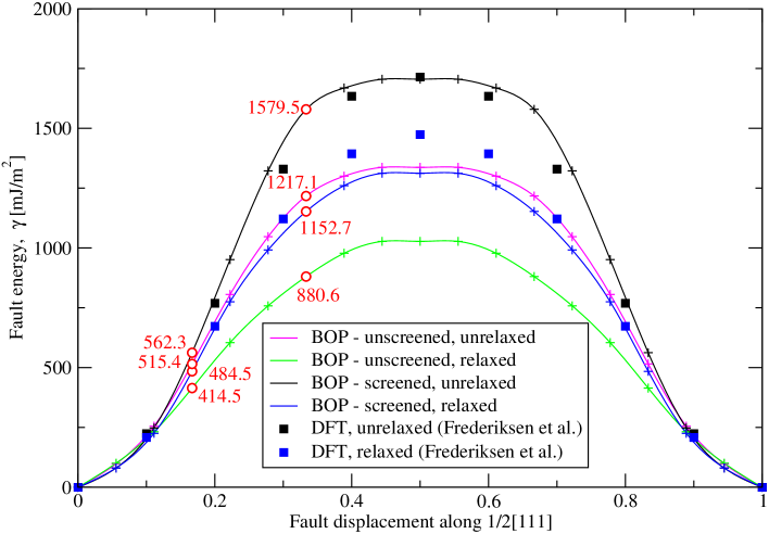
Figure 3.1: $\langle{111}\rangle$ cross-section of $\{110\}$ $\gamma$-surfaces for molybdenum calculated using BOP. The squares correspond to the DFT calculations of Frederiksen and Jacobsen, (2003).

The concept of $\gamma$-surfaces is in the first place invaluable in finding possible metastable stacking faults that play an important role in dislocation dissociation. This can be done by first recognizing that $\boldsymbol{f}=-\nabla\gamma(\boldsymbol{t})$ determines the restoring force of the lattice that tends to destroy the disregistry between the upper and lower part of the crystal. If the $\gamma$-surface displays intermediate minima, it is favorable for the dislocation to split into partial dislocations whose Burgers vectors correspond to these minima, in which case the restoring force would vanish. An example is the splitting of $1/2\langle{110}\rangle$ dislocations into a pair of $1/6\langle{112}\rangle$ Shockley partials in fcc crystals.

$\gamma$-surfaces can be calculated relatively easily by means of atomistic simulations utilizing empirical potentials (Duesbery and Vitek,, 1998) or even using the DFT-based methods (e.g. for bcc transition metals see Frederiksen and Jacobsen, (2003)). For the prediction of the structure of the dislocation core in bcc metals, it is natural to look at the $\langle{111}\rangle$ cross-section of these surfaces, since this is the direction of the Burgers vector of dislocations in this lattice. Since the most densely packed plane in the bcc structure is $\{110\}$ and, as shown below, the screw dislocations spread onto these planes, we have calculated the $[111]$ cross-section of the $\gamma$-surface on the $(\bar{1}01)$ plane using both the BOP with and without screening, and with and without relaxation. The results are shown in Fig. 3.1 together with analogous DFT-based calculations of Frederiksen and Jacobsen, (2003). As we see from Fig. 3.1, no minima appear on the calculated $\gamma$-surface, and, therefore, there are no metastable stacking faults on the $\{110\}$ plane. Similarly, no minima are found on the $\{112\}$ $\gamma$-surface. The same result was obtained in all previous calculations of $\gamma$-surfaces in bcc metals (for reviews see e.g. Duesbery, (1989); Duesbery and Richardson, (1991); Duesbery et al., (2002); Moriarty et al., (2002)), and it is thus likely that the non-existence of metastable stacking faults is a general feature of the bcc structure. This implies that $1/2\langle{111}\rangle$ screw dislocations in molybdenum cannot dissociate into partial dislocations and always preserve their total Burgers vector.

The comparison of the $\gamma$-surfaces calculated using BOP and ab initio is complicated by different characters of the simulation cell in the direction perpendicular to the fault plane. Unlike BOP whose block is effectively infinite in this direction, the DFT-based studies employ a fully periodic simulation cell. This makes no difference when comparing the unrelaxed $\gamma$-surfaces calculated by the two methods, and hence the close agreement between the two shows that the screened BOP reproduces the ab initio results very closely. However, if the atoms are allowed to relax, the periodicity of the cell used in ab initio calculations partially confines the motion of atoms during the relaxation, while no such restriction is imposed on the energy minimization using BOP. Consequently, the difference between the relaxed $\gamma$-surfaces obtained ab initio and using BOP, shown in Fig. 3.1, can be attributed to the incompatibility of the simulation cells in the two methods. Finally, the results also demonstrate that the screened BOP reproduces the ab initio data much more closely than the unscreened BOP, and thus introduction of screening of bond integrals is an essential ingredient of the BOPs; this was also demonstrated on other examples by Mrovec et al., (2004).

a) degenerate core (I, II)                           b) non-degenerate core
Figure 3.2: Schematic illustration of the two types of dislocation cores that obey the three-fold symmetry dictated by the lattice.

Following von Neumann’s principle (von Neumann,, 1885), the symmetry of any physical property of a crystal must include the symmetry elements of the point group of this crystal. Hence, the three-fold symmetric character of $\langle{111}\rangle$ axes dictates that the unstressed cores of $1/2\langle{111}\rangle$ screw dislocations must possess at least the three-fold rotational symmetry. This permits two different types of cores that are shown schematically in Fig. 3.2. Each of the two variants of the degenerate core in Fig. 3.2a can be perceived as a generalized splitting into three fractional dislocations with Burgers vectors $1/6[111]$ on $(\bar{1}01)$, $(0\bar{1}1)$, and $(\bar{1}10)$ planes (Vitek,, 2004). Similarly, the non-degenerate core in Fig. 3.2b can be regarded as a generalized splitting into six fractional dislocations with Burgers vectors $1/12[111]$ on the same planes as above. However, unlike the degenerate core that possesses the minimal symmetry dictated by the von Neumann’s principle, the non-degenerate core is further invariant with respect to the $[\bar{1}01]$ diad. Which type of core is energetically favored can be assessed by comparing the values of the $\gamma$-surface corresponding to the two types of fractional displacements according to the Duesbery-Vitek rule (Duesbery and Vitek,, 1998). In particular, the degenerate core will be preferred if $3\gamma(b/3)<6\gamma(b/6)$, while if the opposite is true the non-degenerate core is favored. From the $\gamma$-surfaces in Fig. 3.1, one can easily verify that both screened and unscreened BOPs predict the existence of the non-degenerate core (see also Mrovec, (2002)).

3.2 Simulation block and structure of the dislocation core

In the following simulations, we use a block of atoms that is oriented such that the $z$-axis coincides with the $[111]$ direction (and thus with the Burgers vector and line direction of the dislocation studied), $y$ is perpendicular to the $(\bar{1}01)$ plane, and $x$ to both $y$ and $z$ such that the coordinate system is right-handed. To simulate an infinitely long straight screw dislocation, we use periodic boundary conditions along the $z$-direction. This reduces the number of $(111)$ atomic layers in the model to three, with the nearest layer-to-layer distance equal to $1/2\sqrt{3}$ in units of the lattice parameter. In our case, the size of the block in the $xy$ plane was about $20\times 20$ lattice parameters.

Starting with an ideal crystal, we inserted a $1/2[111]$ screw dislocation by displacing all atoms in the block according to the elastic anisotropic strain field of the dislocation (Hirth and Lothe,, 1982). The active atoms of the block, shown in Fig. 3.3, were subsequently relaxed using the BOP for molybdenum (Mrovec et al.,, 2004) while holding the atoms in the inert region fixed. The differential displacement map of the relaxed dislocation core is shown in Fig. 3.4. In this projection, the circles stand for atoms in the three successive $(111)$ layers. The lengths of the arrows correspond to the displacements of two neighboring atoms parallel to the Burgers vector, i.e. perpendicular to the plane of the figure, relative to their distance in the perfect lattice. The three longest arrows close to the center of the figure, each corresponding to the relative displacement vector $1/6[111]$ in units of the lattice parameter, define a Burgers circuit that gives $1/2[111]$, the total Burgers vector of the dislocation. The same net product is obtained when going around the six second-largest arrows in the figure, each giving a relative displacement equal to $1/12[111]$, or around any other circuit encompassing the dislocation.

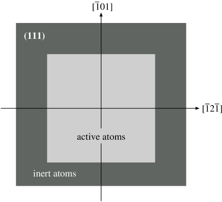
Figure 3.3: The simulated block consists of three $\{111\}$ planes. The dark region extends effectively to infinity.

The dislocation core shown in Fig. 3.4 is non-degenerate, as predicted from the shape of the $\gamma$-surface using the Duesbery-Vitek rule. The core is spread symmetrically on the three $\{110\}$ planes of the $[111]$ zone, namely on the $(\bar{1}01)$ plane whose trace on the $(111)$ plane coincides with the $x$-axis, and on $(0\bar{1}1)$ and $(\bar{1}10)$ planes that both make $60^{\circ}$ with the $(\bar{1}01)$ plane. Due to the non-planar character of the dislocation core, screw dislocations in molybdenum are less mobile than both edge and mixed dislocations, and their motion therefore determines the onset of macroscopic plastic deformation. In order to move the screw dislocation, the applied stress must first transform the core from its initially sessile configuration (Fig. 3.4) into a less symmetric form that can be glissile in the slip plane. Associated with this transformation is a large energy barrier that must be overcome to move the dislocation. This is in contrast to fcc metals and to basal slip in hexagonal crystals, in which screw dislocations, dissociated into Shockley partials, move at low stresses without significant changes in the dislocation core.

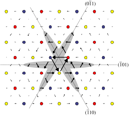
Figure 3.4: Structure of the $1/2[111]$ screw dislocation core calculated using the BOP for molybdenum.

In order to obtain the full information about the motion of the screw dislocation subjected to a general loading, it is first necessary to identify the components of the stress tensor that affect the magnitude of the shear stress parallel to the slip direction at which the dislocation moves. For example, in the case of bcc tantalum, Yang et al., (2001) have shown that ambient hydrostatic pressure causes only marginal changes of the dislocation core and does not affect the stress at which the dislocation moves. However, under extreme conditions such as nuclear explosions or laser-induced shock waves, large hydrostatic stresses may be responsible for significant changes in the electronic structure, and this may no longer be compatible with the interatomic potential.

3.3 Loading by shear stress parallel to the slip direction

For the application of stress the simulated block is divided into two domains, as shown in Fig. 3.3. The atoms in the outer part, called inert atoms, are displaced according the anisotropic strain field corresponding to the applied stress tensor and the long range strain field of the dislocation. The atoms in the inner region, called active atoms, are then relaxed by minimizing the total energy (2.1) of the block. In the first series of simulations, we study the effect of pure shear parallel to the slip direction that exerts a nonzero Peach-Koehler force on the dislocation and thus directly drives its motion.

According to the Schmid law, which is well established in close-packed structures but does not hold in bcc metals, the shear stress parallel to the slip direction in the plane of the slip at which the dislocation starts to move is independent of the orientation of the plane of applied loading. In order to obtain the actual orientation dependence of the critical resolved shear stress (CRSS) parallel to the slip direction at which the dislocation starts to move, we carried out a series of atomistic simulations for different orientations of the plane in which the shear stress parallel to the slip direction is applied. This plane is called the maximum resolved shear stress plane (MRSSP) and its orientation is defined by the angle $\chi$ which it makes with the $(\bar{1}01)$ plane, as shown in Fig. 3.5. Due to the crystal symmetry, it is sufficient to consider only the MRSSPs in the angular region $-30^{\circ}<\chi<+30^{\circ}$. This region is bounded by two $\{112\}$ planes that are twinning planes in bcc crystals. For $\chi<0$, the nearest $\{112\}$ plane, i.e. $(\bar{1}\bar{1}2)$, is sheared in the twinning sense. On the other hand, for $\chi>0$, the nearest $\{112\}$ plane, i.e. $(\bar{2}11)$, is sheared in the antitwinning sense.

The applied stress tensor is given in the right-handed coordinate system with the $y$-axis normal to the MRSSP and $z$ parallel to the slip direction. In this orientation, the stress tensor for the applied shear stress, $\sigma$, parallel to the slip direction acting in the MRSSP is

$$\mathbf{\Sigma}=\left(\begin{array}[]{ccc}0&0&0\\ 0&0&\sigma\\ 0&\sigma&0\end{array}\right)\quad.$$ (3.1)

In the application of stress, we started with a completely relaxed block with the $1/2[111]$ screw dislocation in the middle, as shown in Fig. 3.4. To ensure that the stress at which the dislocation starts to move, the critical resolved shear stress (CRSS), is found with sufficient precision, the shear stress $\sigma$ was built up incrementally in steps of $0.001C_{44}$, where $C_{44}$ is the elastic modulus. In each loading step, the atomic block was fully relaxed before increasing $\sigma$. At low stresses, the dislocation core transforms from its initially sessile, three-fold symmetric non-degenerate core, to a less symmetric form. This transformation is purely elastic in that the block returns into its original configuration when the stress is removed. Once the applied shear stress $\sigma$ attains the CRSS, the transformation is complete, and the dislocation moves through the crystal.

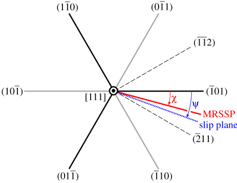
Figure 3.5: Orientation of the planes in the $[111]$ zone.

The obtained dependence of the CRSS on the orientation of the MRSSP, $\chi$, is plotted as circles in Fig. 3.6. For all orientations of the MRSSP, the dislocation moved on the $(\bar{1}01)$ plane, which coincides here with the most highly stressed $\{110\}$ plane of the $[111]$ zone. If the Schmid law were valid in molybdenum, the CRSS would vary with $\chi$ as $\cos^{-1}\chi$, showed as the dashed curve in Fig. 3.6, and all data points in the graph would lie on this curve. In our case, however, the CRSS for antitwinning shear ($\chi>0$) is always higher than the corresponding value for the twinning shear ($\chi<0$). This is the well-known twinning-antitwinning asymmetry that is commonly observed in experiments on many bcc metals and is one evidence of the breakdown of the Schmid law in these materials.

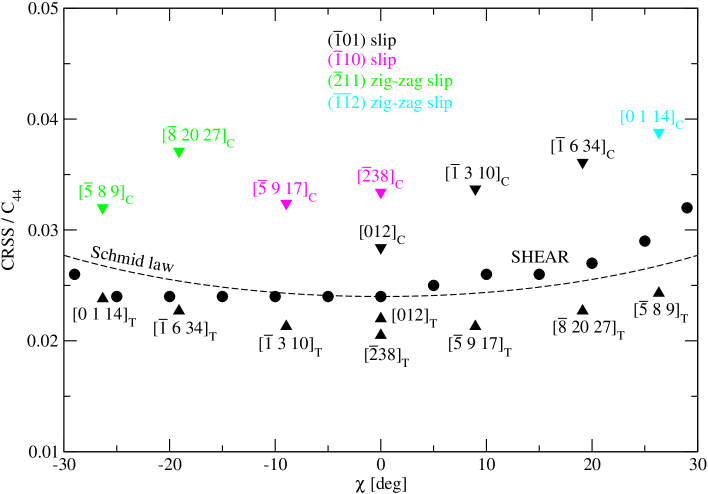
Figure 3.6: Orientation dependence of the CRSS for loading by shear stress parallel to the slip direction (circles), tension (up-triangles), and compression (down-triangles). The circles and up-triangles correspond to slip on the $(\bar{1}01)$ plane; different slip planes for loading in compression are labeled separately.

3.4 Loading in tension and compression

Recall that any uniaxial loading exerts a general triaxial strain state at any point of the loaded body. Therefore, an important test that reveals whether or not the shear stress parallel to the slip direction is the only stress component that affects the dislocation movement is to apply uniaxial loadings in several different orientations and calculate the corresponding CRSS at which the dislocation moves. Due to the symmetry of bcc crystals, the complete set of loading axes can be found within the stereographic triangle shown in Fig. 3.7. For our orientation of the crystal, where $(\bar{1}01)$ is the most highly stressed $\{110\}$ plane of the $[111]$ zone, the three corners of the stereographic triangle of interest coincide with axes $[001]$, $[011]$, $[\bar{1}11]$.

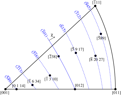
Figure 3.7: Stereographic triangle corresponding to the orientation of the block in which $(\bar{1}01)$ is the most highly stressed $\{110\}$ plane in the zone of the $[111]$ slip direction.

The orientations of the loading axes in tension and compression that were studied are plotted in Fig. 3.7. For any loading axis, one can always find the orientation of the MRSSP in the zone of the $[111]$ slip direction. For the set of chosen orientations, the corresponding MRSSPs are shown in Fig. 3.7 as dashed curves. The shear stress parallel to the slip direction resolved in the MRSSP, which moves the dislocation in tension/compression, is the CRSS that can be directly compared with the value calculated for the same $\chi$ by applying the pure shear stress parallel to the slip direction. In Fig. 3.6, the values of the CRSS for tension are plotted as up-triangles and for compressions as down-triangles. If, for the same $\chi$, the CRSS for tension/compression (triangles) were the same, or very close, to those calculated for pure shear stress parallel to the slip direction (circles), we would conclude that only the shear stress parallel to the slip direction controls the plastic flow of single crystals of bcc molybdenum. However, the observed large deviation of the CRSS for tension/compression from the CRSS for pure shear parallel to the slip direction implies that the motion of the screw dislocation is also affected by other stress component(s).

The analysis described above was performed originally by Ito and Vitek, (2001) using the Finnis-Sinclair potential for molybdenum. They concluded that the shear stresses perpendicular to the slip direction also play role in the dislocation motion and thus in the plastic flow of bcc metals. The analysis in Ito and Vitek, (2001) was confined only to $\chi=0$ and to exactly $\chi=\pm 30^{\circ}$ for which the MRSSP coincides with the highly symmetrical $\{211\}$ planes. In the following section, our objective is to investigate in detail the effect of the shear stress perpendicular to the slip direction and its impact on the magnitude of the CRSS for slip for a number of orientations of the MRSSP.

3.5 Effect of the shear stress perpendicular to the slip direction

Shear stress perpendicular to the slip direction does not exert any Peach-Koehler force (Peach and Koehler,, 1950) on the dislocation and, therefore, cannot cause its movement. However, it plays an important role in the transformation of the dislocation core (Duesbery,, 1989; Vitek,, 1992; Ito and Vitek,, 2001).

3.5.1 Transformation of the dislocation core

The first obvious question is how the dislocation core changes upon applying a pure shear stress perpendicular to the slip direction. Since no shear stress parallel to the slip direction is applied here, it is not appropriate to use the term MRSSP when referring to the plane that defines the orientation of applied loading. The stress tensor applied in the coordinate system where the $y$-axis is normal to the plane defined by the angle $\chi$, and $z$ is parallel to the dislocation line (and the slip direction) now has the following structure:

$$\mathbf{\Sigma}=\left(\begin{array}[]{ccc}-\tau&0&0\\ 0&\tau&0\\ 0&0&0\end{array}\right)\quad.$$ (3.2)

Here, $\tau$ is the magnitude of the shear stress perpendicular to the slip direction that is resolved in this orientation as a combination of two normal stresses. In these simulations, the applied stress was built up in steps of $0.005C_{44}$.

Because the shear stress perpendicular to the slip direction cannot move the dislocation, the deformation exerted by this stress in the crystal is purely elastic. In the following, we will focus on the case $\chi=0$, but the same analysis holds also for other angles $\chi$. The final structure of the dislocation core obtained by relaxing the simulated block at $\tau=\pm 0.05C_{44}$ is shown in Fig. 3.8. For the negative $\tau$, the core constricts on the $(\bar{1}01)$ plane and extends on both $(0\bar{1}1)$ and $(\bar{1}10)$ planes. Due to the larger spreading of the core on the two low-stressed $\{110\}$ planes, this suggests that the dislocation will be easier to move in $(0\bar{1}1)$ or $(\bar{1}10)$ planes than in the $(\bar{1}01)$ plane. On the other hand, for the positive $\tau$, the dislocation core extends on the $(\bar{1}01)$ plane and constricts on both $(0\bar{1}1)$ and $(\bar{1}10)$ planes which suggests that the dislocation will move most easily on the $(\bar{1}01)$ plane. Hence, one can expect that the subsequent loading by the shear stress parallel to the slip direction will move the dislocation in the $(\bar{1}01)$ plane for $\tau>0$, while $(0\bar{1}1)$ and $(\bar{1}10)$ may be the slip planes for $\tau<0$.

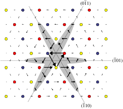
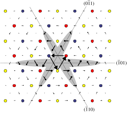
a) $\tau/C_{44}=-0.05$                                            b) $\tau/C_{44}=+0.05$

Figure 3.8: Structure of the dislocation core upon applying (a) negative and (b) positive shear stress perpendicular to the slip direction in the coordinate system for which $\chi=0$.

Besides the preference for slip on a particular $\{110\}$ plane of the $[111]$ zone, the changes in the structure of the dislocation core also suggest how large a CRSS is needed to drive the dislocation glide. For example, assume again that the crystal is loaded by the stress tensor $\mathbf{\Sigma}$ (Eq. 3.2) defined in the coordinate system where the $y$-axis coincides with the normal to the $(\bar{1}01)$ plane. If we apply positive $\tau$, the core extension on the $(\bar{1}01)$ plane makes the glide on this plane easier, as compared to the three-fold symmetric core at zero $\tau$. Hence, one may expect that the ${\rm CRSS}$ at $\tau>0$ will decrease with increasing $\tau$. On the other hand, applying a negative $\tau$ makes the glide on the $(\bar{1}01)$ plane increasingly more difficult and, at larger negative $\tau$, the $(\bar{1}01)$ glide may be suppressed completely. Instead, the dislocation glide may proceed exclusively on one of the other two $\{110\}$ planes of the $[111]$ zone. However, because the shear stress parallel to the slip direction resolved into the planes with $\chi=\pm 60^{\circ}$ is only ${\rm CRSS}/2$, an appreciably larger CRSS for slip of the dislocation can be expected at larger negative $\tau$.

3.5.2 Dependence of the CRSS on the shear stress perpendicular to the slip direction

From the previous text we know that the shear stress perpendicular to the slip direction can make the slip either easier (the core extends further onto the $(\bar{1}01)$ plane) or more difficult (the core extends out of the $(\bar{1}01)$ plane). In order to investigate the dependence of the CRSS on the magnitude of the shear stress $\tau$ perpendicular to the slip direction, we carried out a number of atomistic simulations of the $1/2[111]$ screw dislocation subjected to simultaneous loading by shear stresses perpendicular and parallel to the slip direction. The shear stress parallel to the slip direction was applied in the seven differently oriented MRSSPs for which we have performed the simulations in tension/compression. In each case the shear stress perpendicular to the slip direction (3.2) was first applied in steps, as explained in Section 3.5.1. Keeping the shear stress $\tau$ fixed, we then incrementally built up the shear stress parallel to the slip direction, i.e. the stress tensor (3.1), until the CRSS was attained and the dislocation moved into the next equivalent site. At this point the applied stress tensor reads

$$\mathbf{\Sigma}=\left(\begin{array}[]{ccc}-\tau&0&0\\ 0&\tau&{\rm CRSS}\\ 0&{\rm CRSS}&0\end{array}\right)\quad.$$ (3.3)

Note, that the plane of the maximum shear stress perpendicular to the slip direction is inclined with respect to the MRSSP by the angle $-45^{\circ}$.

For each orientation of the MRSSP, the procedure outlined above was implemented for a number of values of $\tau$, both positive and negative. Without the loss of generality, we will discuss here in detail only three orientations of the MRSSP, namely $(\bar{1}01)$ at $\chi=0$, and $(\bar{3}12)$, $(\bar{2}\bar{1}3)$ at $\chi\approx\pm 19^{\circ}$. However, the complete set of the ${\rm CRSS}-\tau$ dependencies calculated for the seven MRSSPs considered is shown in Fig. 3.9. If the Schmid law were valid, the CRSS would be independent of $\tau$, and for $\chi=0$ the CRSS would be the same as in the case of pure shear parallel to the Burgers vector, specifically $0.024C_{44}$. In contrast, one can observe a strong dependence of the CRSS on the shear stress perpendicular to the slip direction, in particular for negative $\tau$.

a) MRSSP $(\bar{1}01)$, $\chi=0$

b) MRSSP $(\bar{6}15)$, $\chi=+9^{\circ}$ (circles) and $(\bar{5}\bar{1}6)$, $\chi=-9^{\circ}$ (squares)

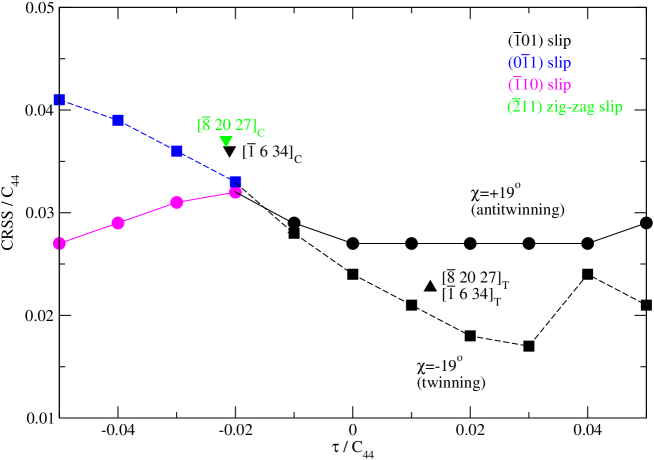
c) MRSSP $(\bar{3}12)$, $\chi=+19^{\circ}$ (circles) and $(\bar{2}\bar{1}3)$, $\chi=-19^{\circ}$ (squares)

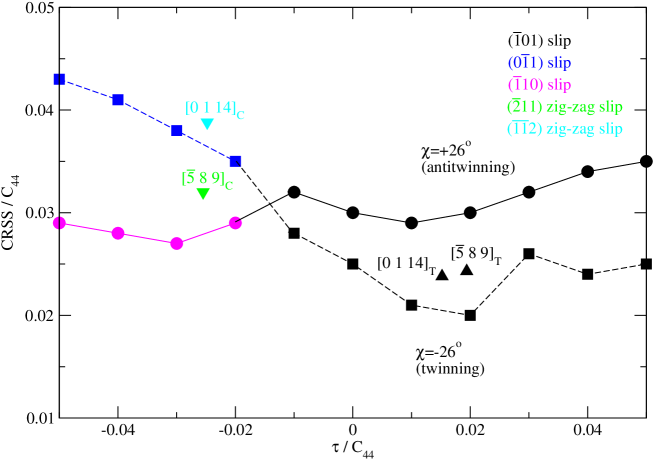
d) MRSSP $(\bar{9}45)$, $\chi=+26^{\circ}$ (circles) and $(\bar{5}\bar{4}9)$, $\chi=-26^{\circ}$ (squares)

Figure 3.9: Dependence of the CRSS on the shear stress perpendicular to the slip direction, $\tau$, for seven studied orientations of the MRSSP.

At positive $\tau$, the CRSS is lower when compared to $\tau=0$, and the slip always occurs on the expected $(\bar{1}01)$ plane with the highest Schmid factor. Because the dislocation core corresponding to positive $\tau$ spreads predominantly on the $(\bar{1}01)$ plane, see Fig. 3.8b, the shear stress perpendicular to the slip direction effectively promotes the dislocation glide by lowering the CRSS required to overcome the barrier for slip on the $(\bar{1}01)$ plane.

In contrast, negative $\tau$ extends the dislocation core out of the $(\bar{1}01)$ plane and thereby makes the slip on this plane more difficult. For values of $\tau/C_{44}>-0.02$, the constriction of the core on the $(\bar{1}01)$ plane is less than its extension on the $(0\bar{1}1)$ or the $(\bar{1}10)$ plane. In this case the slip still proceeds on the expected $(\bar{1}01)$ plane. However, for larger negative values of $\tau$ the extension of the core into the $(0\bar{1}1)$ or the $(\bar{1}10)$ plane becomes significant, and the slip then occurs preferentially on one of these planes. It should be noted that the Schmid factors corresponding to both the $(0\bar{1}1)[111]$ and the $(\bar{1}10)[111]$ slip systems are typically a half of that for the most highly stressed $(\bar{1}01)[111]$ slip system. The occurrence of the slip on these planes is thus reminiscent of the experimentally observed anomalous slip that takes place on the slip systems with very low Schmid factors (Bolton and Taylor,, 1972; Creten et al.,, 1977; Jeffcoat et al.,, 1976; Matsui and Kimura,, 1976; Reed and Arsenault,, 1976).

One can see by examining the ${\rm CRSS}-\tau$ dependencies shown in Fig. 3.9c, that for $\chi=-19^{\circ}$, which is in the regime of the twinning shear on the nearest $\{112\}$ plane, the behavior is similar to that found for $\chi=0$. However, for $\chi=+19^{\circ}$, when shearing on the nearest $\{112\}$ plane is in the antitwinning sense, the ${\rm CRSS}$ is almost independent of $\tau$. The origin in this behavior must be hidden in the effect of $\tau$ on the structure of the dislocation core. Let us consider application of the stress tensor (3.2) defined in the right-handed coordinate system where the $z$-axis is $[111]$ and $y$ is perpendicular to the $(\bar{3}12)$ plane, the MRSSP for $\chi=+19^{\circ}$. Projecting the stress tensor $\mathbf{\Sigma}$ into the coordinate system in which the $y$-axis is perpendicular to $(\bar{1}01)$, $(0\bar{1}1)$ and $(\bar{1}10)$, respectively, one finds that the $(\bar{1}01)$ plane is subjected to the shear stress perpendicular to the slip direction with the magnitude $+0.8\tau$, the $(0\bar{1}1)$ plane, inclined by $-60^{\circ}$ with respect to the $(\bar{1}01)$ plane, to $-0.9\tau$, and the $(\bar{1}10)$ plane, inclined by $+60^{\circ}$ with respect to the $(\bar{1}01)$ plane, to $+0.1\tau$. Note that a positive projected shear stress perpendicular to the slip direction results in an extension of the core in a given $\{110\}$ plane and a negative projected shear to a constriction of the core. Clearly, the dislocation core extends with increasing $\tau$ on both $(\bar{1}01)$ and $(\bar{1}10)$ planes. This competing extension of the core on two different $\{110\}$ planes then effectively inhibits the sessile $\rightarrow$ glissile transformation of the core in the $(\bar{1}01)$ slip plane and results in the observed independence of the CRSS on $\tau$.

Superimposed in Fig. 3.9 are also results for the uniaxial loadings examined earlier in Section 3.4. For loading in tension, the resolved shear stress perpendicular to the slip direction is always positive, while for compression it is always negative. For consistency, we consider here only the deviatoric part of the stress tensor. One can observe a close agreement of the ${\rm CRSS}-\tau$ data calculated for tension/compression (triangles) with the data for combined loading by the shear stress perpendicular and parallel to the slip direction (squares/circles). Because the same agreement is obtained also for all other orientations of the MRSSP, one can conclude that we have identified all stress components that affect screw dislocation glide and thus the plastic deformation of single crystals of molybdenum. These stresses are: (i) shear stress perpendicular to the slip direction that merely changes the structure of the dislocation core but does not drive the glide process, and (ii) shear stress parallel to the slip direction whose critical value (CRSS) determines the onset of the dislocation glide. The concomitant effect of these stress components on the onset of glide of an isolated $1/2[111]$ screw dislocation is given by the calculated ${\rm CRSS}-\tau$ dependencies.

3.6 Prediction of the macroscopic slip plane from atomistics

A number of plastic deformation experiments on pure single crystals of molybdenum and also other refractory metals reveal that, for certain orientations of tensile/compressive axes, the macroscopic slip does not proceed on any of the available $\{110\}$ planes but, instead, on planes of lower symmetry. At first glance, the observation of the slip on a high-index plane appears to disagree with the results of our atomistic simulations in which the $1/2[111]$ screw dislocation always moves by elementary steps on one of the three $\{110\}$ planes of the zone of the slip direction. In the following, we will demonstrate how the elementary microscopic steps of the dislocation on the three $\{110\}$ planes can lead naturally to macroscopic slip on any plane containing the $[111]$ slip direction.

Slip on $\{112\}$ planes is often observed in experiments if the orientation of the MRSSP is close to $\pm 30^{\circ}$, in which case two $\{110\}$ planes become subjected to almost identical shear stresses parallel to the slip direction. In view of the results of atomistic modeling presented earlier, this macroscopically observed $\{112\}$ slip can be understood as a consequence of dislocations moving in a zig-zag fashion by elementary steps on the two most highly stressed $\{110\}$ planes; see Fig. 3.10. Due to the limited resolution in experiments, the individual $\{110\}$ steps cannot be directly observed, and the onset of plastic deformation reveals itself on the macroscopic level by slip traces on the intermediate $\{112\}$ plane.

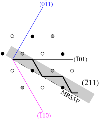
Figure 3.10: Schematic illustration of the $\{112\}$ zig-zag slip by elementary steps of the dislocation on the two adjacent $\{110\}$ planes. The circles represent the positions of atoms and the filled band the macroscopically observed slip trace on the $(\bar{2}11)$ plane.

If the MRSSP does not coincide exactly with any $\pm 30^{\circ}$ plane, one of the two adjacent $\{110\}$ planes will be more stressed than the other, which may result in slip on any high-index plane bounded by the two $\{110\}$ planes. On the microscopic level, this motion corresponds to a particular type of the zig-zag slip in which the dislocation makes more steps on one $\{110\}$ plane than on the other. This slip mode was observed in molybdenum under compression for $\chi=+25^{\circ}$ at the temperature $77~{}{\rm K}$ by Jeffcoat et al., (1976). Two groups of fine slip traces appeared on the surface, one at $\psi\approx+10^{\circ}$ and the other at $\psi\approx+51^{\circ}$, which are close to the $(\bar{1}01)$ and $(\bar{1}10)$ planes that are subjected to the highest shear stresses parallel to the slip direction. A more thorough analysis of the observations of slip traces in single crystals of molybdenum at low temperatures and their correlation with the results of our atomistic studies will be presented in Section 4.7.

Chapter 4 The 0 K effective yield criterion

The opposite of a correct statement is a false statement.

The opposite of a profound truth may well be another profound truth.

Niels Bohr

Based on the atomistic results presented in the previous chapter, we will now formulate a model that generalizes these data to real single crystals containing dislocations of all possible Burgers vectors. We will then proceed to formulate the 0 K effective yield criterion that explicitly involves the effect of shear stresses perpendicular and parallel to the slip direction. The functional form of this criterion follows from the non-associated plastic flow model (Qin and Bassani, 1992a, ; Qin and Bassani, 1992b, ) proposed originally for Ni₃Al. For an exhaustive explanation of the effects of non-Schmid stresses and the related differences between the yield function and the flow potential, refer to Bassani, (1994).

4.1 Model of plastic flow of real single crystals

In order to extend the calculated ${\rm CRSS}-\chi$ and ${\rm CRSS}-\tau$ dependencies to real single crystals at $0~{}{\rm K}$, we will consider that mobile screw dislocations populate all $\{110\}\langle{111}\rangle$ systems. We have seen earlier that the actual slip plane does not necessarily coincide with the most highly stressed $\{110\}$ plane in the zone of the slip direction. For the sake of clarity, we thus define a reference plane as a particular $\{110\}$ plane in the zone of the slip direction from which the angle of the MRSSP, $\chi$, and the angle of the slip plane, $\psi$, are measured. From symmetry, 24 reference systems can be recognized in bcc crystals, each defined by a reference plane and a slip direction, and these are shown in Fig. 4.1. For example, there are three reference planes in the zone of the $[111]$ slip direction, namely $(01\bar{1})$, $(\bar{1}01)$ and $(1\bar{1}0)$.

If we neglect the interactions between dislocations, the motion of each individual dislocation is governed by the same ${\rm CRSS}-\chi$ and ${\rm CRSS}-\tau$ dependencies as those for an isolated $1/2[111]$ dislocation. To apply these dependencies to any reference system $\alpha$, it is first necessary to find the angle $\chi_{\alpha}$ of the MRSSP in the zone of the corresponding $\langle{111}\rangle$ slip direction that lies within the $\pm 30^{\circ}$ angular region measured from the respective $\{110\}$ reference plane. For instance, the MRSSP of the $(\bar{1}01)[111]$ reference system always lies between the $(\bar{1}\bar{1}2)$ plane at $\chi=-30^{\circ}$ and the $(\bar{2}11)$ plane at $\chi=+30^{\circ}$ measured relative to the $(\bar{1}01)$ reference plane, as shown in Fig. 3.5. Furthermore, because the CRSS is always assumed to be positive, we will require that the shear stress parallel to the slip direction resolved in each of these MRSSPs, $\sigma_{\alpha}$, is also positive. It is then a simple task to show that only 4 out of the total of 24 reference systems satisfy both requirements, i.e. $-30^{\circ}<\chi_{\alpha}<+30^{\circ}$ and $\sigma_{\alpha}>0$, and thus only these four systems can be activated for slip by the applied stress. For the opposite sense of loading, the four reference systems are sheared in the opposite sense and thus the relevant systems change to those with the same reference planes as above but opposite slip directions.

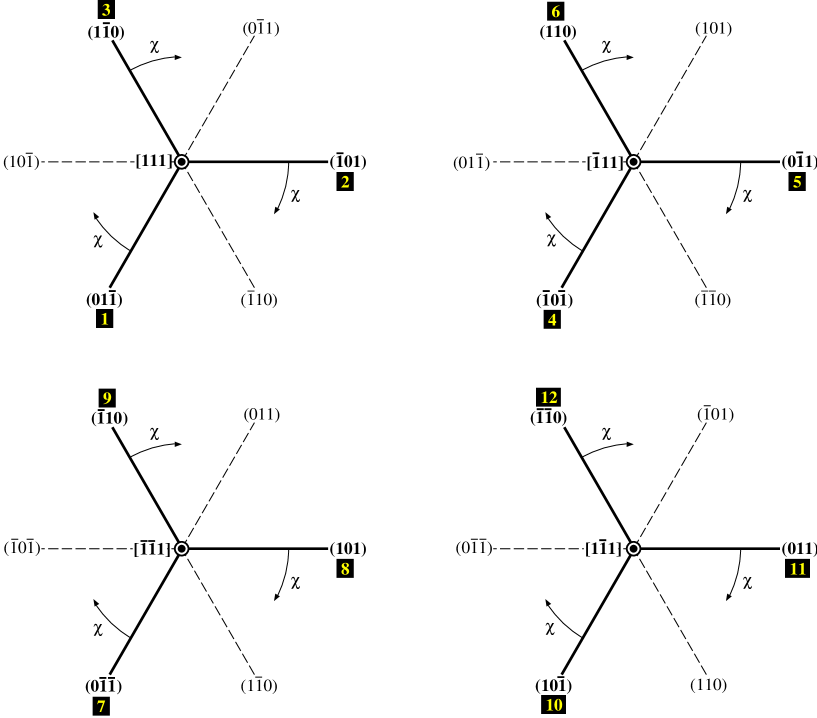
Figure 4.1: Orientations of $\{110\}$ reference planes in the zones of the four $\langle{111}\rangle$ slip directions in bcc crystals corresponding to systems 1 to 12 in Tab. 4.2. The positive sense of $\chi$ in each system is marked relative to the solid lines representing the reference planes. The orientations of MRSSPs in the zones of the opposite slip directions, corresponding to the conjugate systems 13 to 24, can be obtained simply by reversing the sense of $\chi$.

In each loading step and for each of the four reference systems $\alpha$, one can determine the shear stresses perpendicular and parallel to the slip direction applied in each of the four MRSSPs at $\chi_{\alpha}$. This then yields the stress state $(\tau,\sigma)_{\alpha}$ associated with the MRSSP of the system $\alpha$. Since all $1/2\langle{111}\rangle$ dislocations are equivalent, the shear stresses $(\tau,\sigma)_{\alpha}$ for the four $\{110\}\langle{111}\rangle$ systems can now be directly compared with atomistic results for $\chi\approx\chi_{\alpha}$ obtained for the isolated $1/2[111]$ dislocation. Within the framework of this model, a particular system $\alpha$ is activated for slip when $\sigma_{\alpha}$ reaches the CRSS for the given $\tau_{\alpha}$, as determined by the calculated ${\rm CRSS}-\tau$ dependence for the MRSSP defined by angle $\chi_{\alpha}$. From our atomistic simulations, these dependencies are available only for seven orientations of the MRSSP and, therefore, the comparison will be made in the ${\rm CRSS}-\tau$ graph for $\chi_{\alpha}$ that is closest to one of the values from the set $\chi\approx\{0^{\circ},\pm 9^{\circ},\pm 19^{\circ},\pm 26^{\circ}\}$.

In order to demonstrate this transfer of the atomistic results to real single crystals, we will now consider a combined loading by the shear stresses perpendicular and parallel to the $[111]$ slip direction, applied in the MRSSP that coincides with the $(\bar{1}01)$ plane. As an example we choose one particular orientation of the loading axis for which the shear stresses perpendicular and parallel to the slip direction resolved in the MRSSP $(\bar{1}01)$ vary along a straight loading path with the slope $\tau/\sigma\approx 1.5$, see Fig. 4.2a. If the crystal contained only $1/2[111]$ dislocations, the slip would occur when this loading path reaches the CRSS given by the atomistically calculated ${\rm CRSS}-\tau$ dependence, specifically the point “B”. However, in real crystals, all slip systems are stressed simultaneously and the activation of a particular system depends on the interplay between the shear stresses perpendicular and parallel to the slip direction resolved in the corresponding MRSSP. Hence, while the loading evolves along the path in Fig. 4.2a, the two shear stresses resolved in the MRSSP of the $(110)[\bar{1}11]$ reference system follow the path drawn in Fig. 4.2b with the slope $\tau/\sigma\approx 0.5$. Note that the slope of the loading path in the MRSSP is generally different for the two reference systems. As we increase the load, the stress states in the two MRSSPs, in zones of $[111]$ and $[\bar{1}11]$ slip directions, follow their respective loading paths. When the applied loading in Fig. 4.2b reaches the point marked “A”, the $(110)[\bar{1}11]$ system becomes operative. However, at this stress state, the resolved loading in the MRSSP of the $(\bar{1}01)[111]$ system is subcritical in that the corresponding stress state is still well below the calculated CRSS for this system (see Fig. 4.2a). Consequently, the $(110)[\bar{1}11]$ system will become operative first, followed by the operation of the $(\bar{1}01)[111]$ system.

a) loading path $\tau/\sigma\approx 1.5$                       b) loading path $\tau/\sigma\approx 0.5$
Figure 4.2: Evolution of loading in two different $\{110\}\langle{111}\rangle$ systems (lines) induced by shear stresses perpendicular and parallel to the slip direction applied in the $(\bar{1}01)[111]$ system. Squares correspond to the atomistic data calculated for a single $1/2[111]$ dislocation in Section 3.5.2. The points marked ”A” and ”B” in the two panels correspond to the same applied loading.

This simple model demonstrates that the onset of slip in real single crystals can be associated with the stress for which the loading path of any of the four potentially active reference systems, drawn in their respective MRSSPs, reaches the CRSS found in atomistic calculations. Even though $(\bar{1}01)[111]$ may be the most highly stressed system in the sense of the Schmid law, it does not automatically follow that no other slip system can be activated prior to this system. This would only be the case if shear stresses perpendicular to the slip direction did not affect the magnitude of the CRSS, which is clearly not the case in bcc molybdenum. Indeed, even pure shear stress perpendicular to the slip direction of one system can be resolved as shear stress parallel to the slip direction in the MRSSP of a different slip direction, and consequently it can induce glide of dislocations in this system.

4.2 The 0 K effective yield criterion

The theory of non-associated plastic flow in bcc metals, put forward by Qin and Bassani, 1992a ; Qin and Bassani, 1992b , aims at reformulating the plasticity of bcc metals by introducing an effective yield criterion that captures the breakdown of the Schmid law in these materials. As we have seen previously, this is inherently associated with the behavior of individual screw dislocations and, therefore, the results of atomistic simulations presented earlier can be used to obtain the actual form of the effective yield stress. This development has been carried out jointly with V. Racherla and J. Bassani and is explained in more detail in Vitek et al., (2004).

4.2.1 Restricted form

For the sake of clarity, we first construct the so-called restricted form of the effective yield criterion that merely reproduces the dependence of the CRSS on $\chi$ for the case of pure shear stress parallel to the slip direction (circles in Fig. 3.6), i.e. without considering the effect of perpendicular shear stresses. This can be achieved by writing the effective stress, $\tau^{*}$, as a linear combination of shear stresses parallel to the slip direction acting in two distinct planes chosen to be of the $\{110\}$ type,

$$\tau^{*}=\sigma^{(\bar{1}01)}+a_{1}\sigma^{(0\bar{1}1)}\leq\tau^{*}_{cr}\ ,$$ (4.1)

where $a_{1}$ and $\tau_{cr}^{*}$ are parameters that can be determined by fitting the ${\rm CRSS}-\chi$ atomistic results. If $\tau^{*}<\tau^{*}_{cr}$, screw dislocations do not move, and the deformation is purely elastic. However, when $\tau^{*}=\tau^{*}_{cr}$, the applied stress induces the glide of screw dislocations and the crystal is said to yield or flow. In this model, $\tau^{*}_{cr}$ is an effective yield stress that represents the critical value of $\tau^{*}$. Since the $(\bar{1}01)$ plane is the actual slip plane for any orientation of the applied shear stress, $\sigma^{(\bar{1}01)}$ is the Schmid stress. The shear stress $\sigma^{(0\bar{1}1)}$, parallel to the slip direction and acting in the $(0\bar{1}1)$ plane, deforms the dislocation core and thus affects the magnitude of the CRSS at which the dislocation starts to move. This core transformation gives rise to the twinning-antitwinning asymmetry of the CRSS for shear stress parallel to the slip direction that is shown in Fig. 3.6. Without this additional term, Eq. 4.1 reduces to the Schmid law. Note that the choice of the auxiliary stress component, in our case $\sigma^{(0\bar{1}1)}$, is arbitrary, and different choices result in different constants $a_{1}$ but identical overall reproduction of the atomistic data.

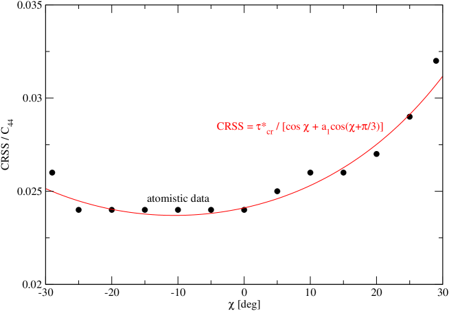
Figure 4.3: Atomistically calculated CRSS for pure shear stress parallel to the slip direction (circles) and the prediction of the effective yield criterion (curve).

The parameters $a_{1}$ and $\tau_{cr}^{*}$ in Eq. 4.1 are determined by fitting the atomistic data for pure shear stress parallel to the slip direction, see Fig. 3.6. For this purpose, it is convenient to rewrite (4.1) in terms of the angle $\chi$ between the MRSSP and the $(\bar{1}01)$ plane. When the applied stress $\sigma$ reaches its critical value, ${\rm CRSS}$, the magnitude of $\tau^{*}$ becomes equal to the effective yield stress, $\tau^{*}_{cr}$, and the criterion reads

$${\rm CRSS}\left[\cos\chi+a_{1}\cos\left(\chi+\frac{\pi}{3}\right)\right]=\tau^{*}_{cr}\ .$$ (4.2)

Each data point $(\chi,{\rm CRSS})$ from Fig. 3.6 thus provides one equation of the type (4.2). The optimal values of $a_{1}$ and $\tau_{cr}^{*}$ are then obtained by the least-squares procedure. In our case, the best fit corresponds to $a_{1}=0.24$ and $\tau_{cr}^{*}/C_{44}=0.027$, where the nonzero value of $a_{1}$ quantifies the degree of the twinning-antitwinning asymmetry observed in atomistic simulations. The quality of this fit is seen in Fig. 4.3.

4.2.2 Full form

The restricted form of the effective yield criterion (4.1) does not capture the effect of shear stresses perpendicular to the slip direction which, as we now know, play an important role in the glide of screw dislocations. In order to reproduce the ${\rm CRSS}-\tau$ dependence found in atomistic calculations, we have to incorporate this dependence into $\tau^{*}$. This can be achieved by complementing $\tau^{*}$ with two additional terms whose coefficients have to be fitted so as to reproduce the ${\rm CRSS}-\tau$ dependence. The full form of the effective yield criterion then reads

$$\tau^{*}=\sigma^{(\bar{1}01)}+a_{1}\sigma^{(0\bar{1}1)}+a_{2}\tau^{(\bar{1}01)}+a_{3}\tau^{(0\bar{1}1)}\leq\tau_{cr}^{*}\ ,$$ (4.3)

where $\sigma$ are shear stresses parallel and $\tau$ shear stresses perpendicular to the slip direction. In this equation, $a_{1}$ and $\tau^{*}_{cr}$ are taken to be the same as the values obtained from the restricted model and, therefore, only $a_{2}$ and $a_{3}$ have to be determined by fitting the ${\rm CRSS}-\tau$ data for the combination of the shear stresses perpendicular and parallel to the slip direction. Similarly as above, it is convenient to rewrite Eq. 4.3 for the case when the applied stress $\sigma$ reaches its critical value, CRSS, and thus $\tau^{*}=\tau^{*}_{cr}$:

$${\rm CRSS}\left[\cos\chi+a_{1}\cos\left(\chi+\frac{\pi}{3}\right)\right]+\tau\left[a_{2}\sin 2\chi+a_{3}\cos\left(2\chi+\frac{\pi}{6}\right)\right]=\tau^{*}_{cr}\ .$$ (4.4)

For each point in the ${\rm CRSS}-\tau$ graph corresponding to an angle $\chi$, we thus obtain an equation for two unknowns, $a_{2}$ and $a_{3}$. Since the number of points in all ${\rm CRSS}-\tau$ graphs greatly exceeds the number of unknowns, the corresponding least-squares fitting is far from unique. However, for all orientations of uniaxial loading studied here, the corresponding shear stresses perpendicular to the slip direction are within $-0.02<\tau/C_{44}<+0.02$ when the CRSS has been attained. Therefore, we have determined $a_{2}$ and $a_{3}$ by fitting only to those points in the ${\rm CRSS}-\tau$ graphs that are within this interval of $\tau$ values, where the ${\rm CRSS}-\tau$ dependence is approximately linear.

We have found that the best fit is obtained when considering only three orientations of the MRSSP, namely $\chi=0$ and $\chi\approx\pm 9^{\circ}$. In each of these planes, only the data for $\tau/C_{44}=\pm 0.01$ were taken into account, since only two points are necessary to specify a slope of the straight line. However, even in this case, the system of 6 algebraic equations for 2 unknowns is overdetermined, and, therefore, the values of $a_{2}$ and $a_{3}$ have been found by least-squares fitting of Eq. 4.4. Finally, note that, since $\tau^{*}$ is linearly dependent on the shear stress perpendicular to the slip direction, the criterion is not capable of reproducing the ${\rm CRSS}-\tau$ dependencies at $|\tau/C_{44}|>0.02$. However, this is not a problem when applying the criterion to study plastic behavior of real single crystals, since for large values of $\tau$ another $\{110\}\langle{111}\rangle$ system always becomes operative before activating the $(\bar{1}01)[111]$ system (see e.g. Fig. 4.2). In other words, straight loading paths for large ratios of $|\tau/\sigma|$ always correspond to orientations that lie outside the stereographic triangle for the $(\bar{1}01)[111]$ system, and, therefore, another $\{110\}\langle{111}\rangle$ system becomes active.

The best fit to the atomistic data obtained by the procedure outlined above yields $a_{2}\approx 0$ and $a_{3}=0.35$. The fact that $a_{2}$ is zero implies that $\tau^{*}$ is independent of the shear stress perpendicular to the slip direction applied in the $(\bar{1}01)$ plane by the stress tensor (3.2). This is clearly a coincidence and not any basic rule, since one can choose a different combination of the two shear stresses perpendicular to the slip direction for which both $a_{2}$ and $a_{3}$ will be nonzero. In summary, the effective yield criterion for molybdenum obtained by fitting the 0 K atomistic data is given by Eq. 4.3 with the parameters summarized in Tab. 4.1.

Table 4.1: Coefficients of the effective yield criterion (4.3) for molybdenum.

$a_{1}$	$a_{2}$	$a_{3}$	$\tau^{*}_{cr}/C_{44}$
0.24	0	0.35	0.027

If the $\tau^{*}$ criterion is to be employed in large-scale simulations, such as finite-element calculations, it has to be sufficiently simple so that efficient calculations of $\tau^{*}$ at every node of the finite-element mesh can be performed. Moreover, yield criteria are used not only to check whether the plastic deformation takes place but often also to predict the magnitude of the stress (e.g. CRSS) at which the yielding occurs. It then follows that $\tau^{*}$ has to be written in a form that can be easily inverted to get the CRSS as a function of other parameters. We have demonstrated that both requirements above are easily satisfied by the linear $\tau^{*}$ criterion (4.3), which provides a relatively simple expression for the CRSS that follows from Eq. 4.4.

4.3 Onset of plastic flow in real single crystals

The full form of the effective yield criterion (4.3) can be directly employed to obtain the ${\rm CRSS}-\tau$ dependencies for real single crystals of molybdenum in which any $\{110\}\langle{111}\rangle$ system may be potentially operative. These dependencies will generalize the ${\rm CRSS}-\tau$ data displayed in Fig. 3.9 that correspond to the glide of a dislocation with a specific Burgers vector, $1/2[111]$.

For any loading, the primary system and the corresponding magnitude of critical loading can be found by: (i) identifying the four reference systems $\alpha$ that can become operative under this loading, (ii) calculating the orientations $\chi_{\alpha}$ of the MRSSPs in zones of these slip directions, and (iii) resolving the shear stresses perpendicular ($\tau_{\alpha}$) and parallel ($\sigma_{\alpha}$) to the slip direction in the MRSSP at $\chi_{\alpha}$. Similarly as in Fig. 4.2, these shear stresses then define a straight loading path in the ${\rm CRSS}-\tau$ graph of the MRSSP at $\chi_{\alpha}$, whose slope is $\eta_{\alpha}=\tau_{\alpha}/\sigma_{\alpha}$. Hence, one can express the CRSS in this system from Eq. 4.4 as

$${\rm CRSS}_{\alpha}=\frac{\tau^{*}_{cr}}{\cos\chi_{\alpha}+a_{1}\cos(\chi_{\alpha}+\pi/3)+\eta_{\alpha}[a_{2}\sin 2\chi_{\alpha}+a_{3}\cos(2\chi_{\alpha}+\pi/6)]}\ ,$$ (4.5)

where the term with $a_{2}$ is retained for generality but vanishes for molybdenum. These calculations yield a set of four values of ${\rm CRSS}_{\alpha}$ in four MRSSPs at $\chi_{\alpha}$ corresponding to different reference systems. In order to compare the prominence of these systems, we project the three stresses ${\rm CRSS}_{\alpha}$ for systems other than $(\bar{1}01)[111]$ into the ${\rm CRSS}-\tau$ graph that corresponds to the MRSSP for the $(\bar{1}01)[111]$ reference system. This yields four critical points that correspond to the activation of slip in the four reference systems. The point on the straight loading path emanating from the origin of the ${\rm CRSS}-\tau$ graph that is closest to the origin marks the stress that causes operation of the primary $\{110\}\langle{111}\rangle$ system or, equivalently, the stress at which a real crystal starts to deform plastically. This analysis can be carried out for many different loading paths in a number of MRSSPs, which yields a set of critical points corresponding to the activation of individual systems. The inner envelope of these lines is then a projection of the 0 K yield surface.

a) $\chi=0$, MRSSP $(\bar{1}01)$

b) $\chi=-19^{\circ}$, MRSSP $(\bar{2}\bar{1}3)$

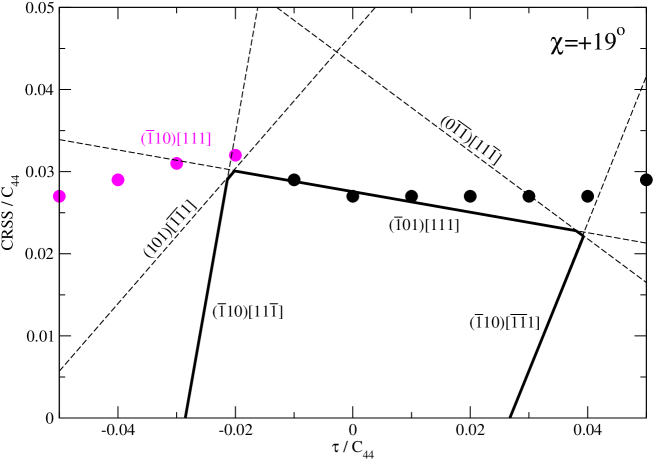
c) $\chi=+19^{\circ}$, MRSSP $(\bar{3}12)$

Figure 4.4: Critical lines for various MRSSPs of the $(\bar{1}01)[111]$ reference system, calculated from the $\tau^{*}$ criterion. The lower panels show the comparison of the shape of the yield surface obtained from the $\tau^{*}$ criterion and that predicted by the Schmid law.

The critical lines marking the onset of activation of the four reference systems $\alpha$, predicted using the procedure described above, are plotted for $\chi=0$ in Fig. 4.4a and for $\chi=\pm 19^{\circ}$ in Fig. 4.4b,c. If the magnitude of the shear stress perpendicular to the slip direction is small, roughly $|\tau/C_{44}|<0.02$, the primary slip system coincides with the most highly stressed $(\bar{1}01)[111]$ system. However, as $|\tau|$ becomes larger, another $\{110\}\langle{111}\rangle$ system becomes dominant when the loading path intersects the corresponding critical line. Since the values of $\tau$ at which the plastic deformation of real crystals takes place are bounded by the yield polygon, $|\tau/C_{44}|$ can never be larger than about $0.03$. If the loading path reaches the corner of the inner polygon generated by the critical lines for the primary slip systems, more systems become activated simultaneously and a multiple slip occurs.

For illustration, we also show by dashed lines in the lower plots of Fig. 4.4a-c how the projection of the yield surface looks if the $\tau^{*}$ criterion reduces to the Schmid law. In this case, the CRSS for the most highly stressed $(\bar{1}01)[111]$ system is clearly independent of $\tau$, and its magnitude follows the Schmid law, i.e. it varies as $1/\cos\chi$. At larger $\tau$, the yield polygon is bounded by the critical lines that correspond to different reference systems than $(\bar{1}01)[111]$. However, it is very important to emphasize that this does not mean that the CRSS is a function of $\tau$ at large $\tau$. The slope of the critical lines for systems other than $(\bar{1}01)[111]$ is obtained purely by the projection of the CRSS from the MRSSPs of these other systems. Without the influence of non-glide stresses, the yield polygons for positive and negative $\chi$ are mirror images of each other. Moreover, since the $(\bar{1}01)$ plane is a mirror plane in bcc crystals, the yield surface projected in the ${\rm CRSS}-\tau$ plot for $\chi=0$ is completely symmetrical with respect to $\tau=0$. All these symmetries are clearly broken in molybdenum as a result of twinning-antitwinning asymmetry and the strong effect of the shear stresses perpendicular to the slip direction.

4.4 Tensorial form of the effective yield criterion

The full form of the effective yield criterion (4.3) can be written in tensorial representation, where one uses directly the crystallographic indices and the stress tensor of applied loading. In a matrix notation, the $\tau^{*}$ criterion reads

$$\tau^{*\alpha}={\bf m}^{\alpha}{\bf\Sigma}^{c}{\bf n}^{\alpha}+a_{1}{\bf m}^{\alpha}{\bf\Sigma}^{c}{\bf n}_{1}^{\alpha}+a_{2}({\bf n}^{\alpha}\times{\bf m}^{\alpha}){\bf\Sigma}^{c}{\bf n}^{\alpha}+a_{3}({\bf n}_{1}^{\alpha}\times{\bf m}^{\alpha}){\bf\Sigma}^{c}{\bf n}_{1}^{\alpha}\leq\tau_{cr}^{*}\ ,$$ (4.6)

where ${\bf\Sigma}^{c}$ is the stress tensor expressed in the $[100],[010],[001]$ cube coordinate system, and $\alpha$ is one of the 24 reference systems in bcc crystals listed in Tab. 4.2.

For a particular $\{110\}\langle{111}\rangle$ reference system, ${\bf m}^{\alpha}$ is a unit vector defining the slip direction, ${\bf n}^{\alpha}$ a unit vector perpendicular to the reference plane, and ${\bf n}_{1}^{\alpha}$ a unit vector perpendicular to the $\{110\}$ plane in the zone of ${\bf m}^{\alpha}$ that makes angle $-60^{\circ}$ with the reference plane. For example, if the reference system considered is $(\bar{1}01)[111]$, the three unit vectors are ${\bf m}^{\alpha}=[111]/\sqrt{3}$, ${\bf n}^{\alpha}=[\bar{1}01]/\sqrt{2}$, ${\bf n}_{1}^{\alpha}=[0\bar{1}1]/\sqrt{2}$. The complete list of the three crystallographic vectors of all $\{110\}\langle{111}\rangle$ systems is given in Tab. 4.2. Notice that the systems labeled 13 to 24 are conjugate to the systems numbered 1 to 12. A pair of systems $\alpha$ and $\alpha+12$ have identical normal of the reference plane, ${\bf n}^{\alpha}$, opposite slip directions ${\bf m}^{\alpha}$, and complementary non-glide plane normals ${\bf n}_{1}^{\alpha}$.

For any applied loading described by the stress tensor ${\bf\Sigma}^{c}$, one can determine the activity of individual reference systems by calculating $\tau^{*\alpha}$ for $\alpha$ from 1 to 24. The slip is activated on a particular system $\alpha$ when the magnitude of $\tau^{*\alpha}$ reaches the effective yield stress, $\tau_{cr}^{*}$. In the framework of the $\tau^{*}$ criterion, the plastic deformation of a single crystal of molybdenum at 0 K commences when the largest of the 24 values of $\tau^{*\alpha}$ reaches the effective yield stress. The corresponding system $\alpha$ is then called the primary system.

Table 4.2: The 24 slip systems in bcc crystals. Note, that the crystallographic vectors ${\bf m}^{\alpha}$, ${\bf n}^{\alpha}$, ${\bf n}_{1}^{\alpha}$ have to be normalized before their use in Eq. 4.6.

$\alpha$	$\rm{ref.\ system}$	${\bf m^{\alpha}}$	${\bf n^{\alpha}}$	${\bf n_{1}^{\alpha}}$	$\alpha$	$\rm{ref.\ system}$	${\bf m^{\alpha}}$	${\bf n^{\alpha}}$	${\bf n_{1}^{\alpha}}$
1	($01\bar{1}$)[$111$]	[$111$]	[$01\bar{1}$]	[$\bar{1}10$]	13	($01\bar{1}$)[$\bar{1}\bar{1}\bar{1}$]	[$\bar{1}\bar{1}\bar{1}$]	[$01\bar{1}$]	[$10\bar{1}$]
2	($\bar{1}01$)[$111$]	[$111$]	[$\bar{1}01$]	[$0\bar{1}1$]	14	($\bar{1}01$)[$\bar{1}\bar{1}\bar{1}$]	[$\bar{1}\bar{1}\bar{1}$]	[$\bar{1}01$]	[$\bar{1}10$]
3	($1\bar{1}0$)[$111$]	[$111$]	[$1\bar{1}0$]	[$10\bar{1}$]	15	($1\bar{1}0$)[$\bar{1}\bar{1}\bar{1}$]	[$\bar{1}\bar{1}\bar{1}$]	[$1\bar{1}0$]	[$0\bar{1}1$]
4	($\bar{1}0\bar{1}$)[$\bar{1}11$]	[$\bar{1}11$]	[$\bar{1}0\bar{1}$]	[$\bar{1}\bar{1}0$]	16	($\bar{1}0\bar{1}$)[$1\bar{1}\bar{1}$]	[$1\bar{1}\bar{1}$]	[$\bar{1}0\bar{1}$]	[$01\bar{1}$]
5	($0\bar{1}1$)[$\bar{1}11$]	[$\bar{1}11$]	[$0\bar{1}1$]	[$101$]	17	($0\bar{1}1$)[$1\bar{1}\bar{1}$]	[$1\bar{1}\bar{1}$]	[$0\bar{1}1$]	[$\bar{1}\bar{1}0$]
6	($110$)[$\bar{1}11$]	[$\bar{1}11$]	[$110$]	[$01\bar{1}$]	18	($110$)[$1\bar{1}\bar{1}$]	[$1\bar{1}\bar{1}$]	[$110$]	[$101$]
7	($0\bar{1}\bar{1}$)[$\bar{1}\bar{1}1$]	[$\bar{1}\bar{1}1$]	[$0\bar{1}\bar{1}$]	[$1\bar{1}0$]	19	($0\bar{1}\bar{1}$)[$11\bar{1}$]	[$11\bar{1}$]	[$0\bar{1}\bar{1}$]	[$\bar{1}0\bar{1}$]
8	($101$)[$\bar{1}\bar{1}1$]	[$\bar{1}\bar{1}1$]	[$101$]	[$011$]	20	($101$)[$11\bar{1}$]	[$11\bar{1}$]	[$101$]	[$1\bar{1}0$]
9	($\bar{1}10$)[$\bar{1}\bar{1}1$]	[$\bar{1}\bar{1}1$]	[$\bar{1}10$]	[$\bar{1}0\bar{1}$]	21	($\bar{1}10$)[$11\bar{1}$]	[$11\bar{1}$]	[$\bar{1}10$]	[$011$]
10	($10\bar{1}$)[$1\bar{1}1$]	[$1\bar{1}1$]	[$10\bar{1}$]	[$110$]	22	($10\bar{1}$)[$\bar{1}1\bar{1}$]	[$\bar{1}1\bar{1}$]	[$10\bar{1}$]	[$0\bar{1}\bar{1}$]
11	($011$)[$1\bar{1}1$]	[$1\bar{1}1$]	[$011$]	[$\bar{1}01$]	23	($011$)[$\bar{1}1\bar{1}$]	[$\bar{1}1\bar{1}$]	[$011$]	[$110$]
12	($\bar{1}\bar{1}0$)[$1\bar{1}1$]	[$1\bar{1}1$]	[$\bar{1}\bar{1}0$]	[$0\bar{1}\bar{1}$]	24	($\bar{1}\bar{1}0$)[$\bar{1}1\bar{1}$]	[$\bar{1}1\bar{1}$]	[$\bar{1}\bar{1}0$]	[$\bar{1}01$]

4.5 The yield surface and effect of non-glide stresses

Any stress state can be represented in the so-called principal space in which the orientations of the three principal axes are the eigenvectors of the stress tensor of the applied loading. The eigenvalues of this stress tensor then give a triad of the so-called principal stresses that define a position in the principal space corresponding to a particular stress state exerted at a point in the loaded body. The locus of the stress states that induce irreversible plastic deformation then characterizes the so-called yield surface which is of a fundamental importance in predictions of the reliability of structural components.

For the sake of clarity, the yield surface is often plotted as a projection of its three-dimensional variant onto the so-called $\pi$-plane whose normal is defined by the three Euler angles $\phi=\psi=0.7854$, $\theta=0.9553$. Because small hydrostatic stresses encountered in engineering applications do not affect the magnitude of the yield stress, we consider the applied stress tensor to be a pure deviator

$$\boldsymbol{\Sigma^{\pi}}=\left[\begin{array}[]{ccc}\sigma_{1}&0&0\\ 0&\sigma_{2}&0\\ 0&0&-\sigma_{1}-\sigma_{2}\end{array}\right]$$ (4.7)

that is applied in a particular orientation in the principal space that corresponds to the three Euler angles $(\phi,\theta,\psi)$. In order to calculate the yield surface, we choose a set of loading paths described by angles $-\pi\leq\zeta\leq\pi$, emanating from the origin in Fig. 4.5. Each of these paths constitutes a well-defined orientation of loading for which we can write the two principal stresses as $\sigma_{1}=\cos\zeta$ and $\sigma_{2}=\sin\zeta$. This determines the applied stress tensor (4.7) that is further transformed into the cube coordinate system to arrive at $\boldsymbol{\Sigma}^{c}$, used in Eq. 4.6. For every reference system $\alpha$ from Tab. 4.2 and the corresponding unit vectors $\boldsymbol{m}^{\alpha}$, $\boldsymbol{n}^{\alpha}$ and $\boldsymbol{n}_{1}^{\alpha}$, Eq. 4.6 provides the effective stress $\tau^{*\alpha}$. From the $\tau^{*}$ criterion, the reference system $\alpha$ becomes activated when $\tau^{*\alpha}$ reaches $\tau^{*}_{cr}$, i.e. when the applied loading increases $k^{\alpha}=\tau^{*}_{cr}/\tau^{*\alpha}$ times. This corresponds to loading by principal stresses $\sigma_{1}^{\alpha}=k^{\alpha}\sigma_{1}$ and $\sigma_{2}^{\alpha}=k^{\alpha}\sigma_{2}$ that provides a set of yield points $(\sigma_{1}^{\alpha},\sigma_{2}^{\alpha})$ marked along the loading path in Fig. 4.5 by circles, which correspond to the activation of individual systems $\alpha$. Note that the point closest to the origin (filled circle) determines a stress state that causes activation of the primary system. When the procedure outlined above is performed for a number of angles $\zeta$, the inner envelope of the yield points generates the $\pi$-plane projection of the yield surface for molybdenum that is shown in Fig. 4.5 as a solid polygon.

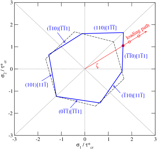
Figure 4.5: Projection of the yield surface generated by the $\tau^{*}$ criterion (4.6) for $a_{1}=0.24$, $a_{2}=0$, $a_{3}=0.35$, $\tau^{*}_{cr}/C_{44}=0.027$ (solid line). Only the deviatoric component of the stress tensor is considered. The $\{110\}\langle{111}\rangle$ primary slip systems that become activated when the loading path reaches the corresponding edge of the solid yield polygon are marked. The dashed Tresca hexagon corresponds to the purely Schmid behavior, i.e. $a_{1}=a_{2}=a_{3}=0$.

For comparison, we also plot in Fig. 4.5 by dashed lines the projection of the yield surface that is generated by the Schmid law, i.e. when $a_{1}=a_{2}=a_{3}=0$. In this case, the yield criterion reduces to that of Tresca whose $\pi$-plane projection is the regular hexagon. The marked difference between the shapes of the two polygons in Fig. 4.5 is the result of the effect of non-glide stresses that are clearly responsible for the asymmetry between the positive and negative loading along a given direction. This asymmetry is most noticeable when $\sigma_{1}=\sigma_{2}$ (i.e. $\zeta=45^{\circ}$) in which case the yield locus at negative stresses coincides with a corner of the Tresca hexagon, while at positive stresses larger elastic deformation is permitted prior to yielding than that predicted by the Schmid law.

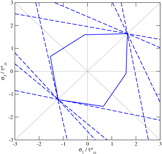
Figure 4.6: $\pi$-plane projection of the yield polygon for molybdenum showing all potentially active slip systems. The dashed lines correspond to various slip systems that become operative if the loading path intersects the yield polygon at its corner.

If the loading path, defined by a pair of principal stresses $(\sigma_{1},\sigma_{2})$, intersects one of the edges of the polygon, the plastic deformation proceeds by single slip on the plane that is marked in the figure. In contrast, if the loading path reaches the yield polygon at one of its corners at which $\sigma_{1}=\sigma_{2}$, many slip systems are typically activated at once, and the plastic deformation proceeds by so-called multislip. This is shown graphically in Fig. 4.6, where the dashed lines correspond to all slip systems that can become activated for slip if the loading path reaches the yield surface at its corner. For comparison, if the plastic deformation of bcc molybdenum were governed by the Schmid law, all edges of the yield polygon that are not parallel to the diagonal ($\sigma_{1}=\sigma_{2}$) would be shared by two different slip systems. One can thus clearly see from Fig. 4.6, that non-glide stresses not only modify the shape of the yield surface, but they are also responsible for the confinement of the multislip to the corners of the yield polygon.

4.6 Primary slip systems in uniaxial loading

We are now in the position to investigate the activity of all $\{110\}\langle{111}\rangle$ systems for any orientation within any stereographic triangle, e.g. that shown in Fig. 3.7 corresponding to the $(\bar{1}01)[111]$ system. This requires identification of the four slip systems $\alpha$ that can become operative and subsequent calculations of the orientations of their MRSSPs, $\chi_{\alpha}$, with the corresponding shear stresses perpendicular and parallel to the slip direction, $\tau_{\alpha}$ and $\sigma_{\alpha}$, respectively. The tensorial expression of the yield criterion (4.6) provides a way of deciding the activity of individual systems and can be used directly to predict the primary slip system for various orientations of uniaxial loading. If one considers a unit loading $\hat{\sigma}_{ax}$ (+1 for tension, -1 for compression) with the axis along a chosen direction and determines the corresponding magnitude of $\tau^{*\alpha}$ for every system $\alpha$, the magnitude of the uniaxial stress for which a system $\alpha$ is activated can be determined as $\sigma_{ax}^{\alpha}=k^{\alpha}\hat{\sigma}_{ax}$ where $k^{\alpha}=\tau^{*}_{cr}/\tau^{*\alpha}$. The stress $\sigma^{\alpha}_{ax}$ corresponding to the highest $\tau^{*\alpha}$, calculated among the four systems, defines the actual uniaxial yield stress and $\alpha$ the corresponding primary system.

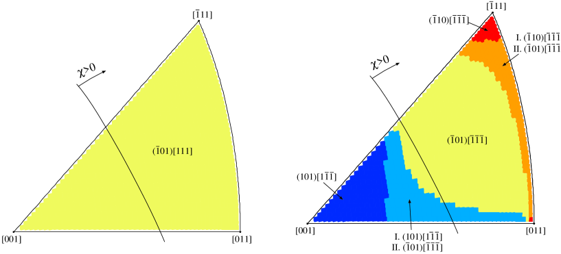
a) tension                                                         b) compression

Figure 4.7: Primary slip systems for uniaxial loading predicted from the effective yield criterion (4.6). In the regions of simultaneous activity of two slip systems, the primary slip system with lower yield stress is marked as “I” and the secondary, whose yield stress is at most 2% higher than I, as “II”.

The primary slip systems in both tension and compression, identified by the $\tau^{*}$ criterion, are shown in Fig. 4.7. In tension, $(\bar{1}01)[111]$ is the primary slip system for any orientation of the loading axis within the standard stereographic triangle. This can be easily understood by looking at the distribution of the critical lines plotted in Fig. 4.4. In tension (positive $\tau$) the ratio of the shear stresses perpendicular and parallel to the slip direction resolved in the MRSSP, $\eta=\tau/\sigma$, is always positive and small enough such that the loading path plotted in the ${\rm CRSS}-\tau$ projection first reaches the critical line for the operation of the $(\bar{1}01)[111]$ system. The slip on other systems is also possible, but at larger stresses than those for which the primary $(\bar{1}01)[111]$ system becomes operative.

In compression (negative $\tau$), the map of primary slip systems for different loading directions is more complex. Because the sense of shearing is now reversed, the slip system with the highest positive Schmid stress is not $(\bar{1}01)[111]$, as in tension, but its conjugate $(\bar{1}01)[\bar{1}\bar{1}\bar{1}]$. In the central region of the triangle, the most operative slip system is, indeed, $(\bar{1}01)[\bar{1}\bar{1}\bar{1}]$. As the loading axis deviates towards the $[011]-[\bar{1}11]$ edge, the $(\bar{1}10)[\bar{1}\bar{1}\bar{1}]$ system becomes increasingly more prominent. There exists a region in which the two systems are equally operative, i.e. the uniaxial yield stress of the secondary system (marked as II) is within 2% from that of the primary system (denoted as I). In this case, both systems operate simultaneously, which may give rise to the macroscopic slip on the $(\bar{2}11)$ plane. For orientations close to the $[\bar{1}11]$ corner, the dislocation moves by single slip on the $(\bar{1}10)[\bar{1}\bar{1}\bar{1}]$ system. A similar situation arises on the other side of the triangle for orientations closer to the $[001]$ corner. Two slip systems have again the same prominence, namely $(\bar{1}01)[\bar{1}\bar{1}\bar{1}]$ and $(101)[1\bar{1}\bar{1}]$. However, since the slip directions are now Burgers vectors of two different dislocations, $1/2[111]$ and $1/2[\bar{1}11]$, these dislocations move simultaneously. This so-called multislip mechanism of plastic deformation was frequently observed in low-temperature experiments, not only on molybdenum but also on all other bcc refractory metals of high purity. For loading axes close to the $[001]$ corner of the standard triangle, the plastic deformation is dominated by the $(101)[1\bar{1}\bar{1}]$ system and single slip on this system ensues.

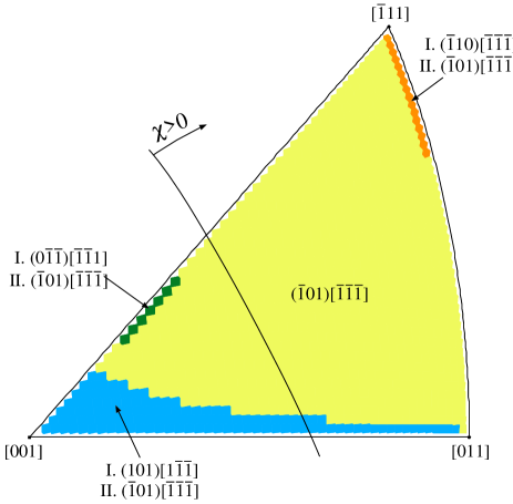
Figure 4.8: Primary slip systems for loading in compression predicted from the Schmid law that arises if the $a_{1}$,$a_{2}$,$a_{3}$ in the effective yield criterion (4.6) are all zero. In the regions of simultaneous activity of two slip systems, the primary slip system with lower yield stress is marked as “I” and the secondary, whose yield stress is at most 2% higher than I, as “II”.

For comparison, we show in Fig. 4.8 the hypothetical distribution of the most operative slip systems for loading in compression dictated by the Schmid law, i.e. when $\tau^{*}$ is equal to the Schmid stress and $a_{1}=a_{2}=a_{3}=0$. In this case, the region of single slip on the $(\bar{1}01)[\bar{1}\bar{1}\bar{1}]$ system occupies most of the stereographic triangle, and only in the three narrow domains close to the corners or edges of the triangle this system operates together with another $\{110\}\langle{111}\rangle$ system. Comparing Fig. 4.8 with Fig. 4.7b, we can conclude that for compression the non-glide stresses are responsible for a substantial broadening of the regions of multiple slip with the single $(\bar{1}01)[\bar{1}\bar{1}\bar{1}]$ system confined to the center of the stereographic triangle.

4.7 Comparisons with low-temperature experiments

In the following, we will show that the effective yield criterion (4.6) correctly reproduces the activity of the slip systems whose traces are observed in low-temperature plastic deformation experiments. We will focus on a characteristic sample of experiments on ultra-high purity single crystals and dilute alloys done at temperatures up to 77 K.

4.7.1 Experiments in pure shear

Due to their inherent experimental complexities, the plastic flow experiments in which the loading is applied as a pure shear are rather rare. A classical study was carried out by Guiu, (1969), who applied the shear at temperatures ranging from $77~{}{\rm K}$ to room temperature such that the MRSSPs were $\{110\}$ and/or $\{112\}$ planes. At 77 K, the experiments revealed a significant twinning-antitwinning asymmetry for shearing on $(\bar{2}11)$ and $(\bar{1}\bar{1}2)$ planes, respectively. At higher temperatures, the difference between the twinning and antitwinning shear diminished. For $\{110\}$ and $\{112\}$ as the MRSSPs, the primary slip plane was always $(\bar{1}01)$. This observation is in a good agreement with the results of atomistic simulations, particularly with Fig. 3.6, in which the slip plane corresponding to pure shear parallel to the slip direction is always the $(\bar{1}01)$ plane with the highest Schmid stress.

4.7.2 Experiments in tension

The prediction of the $\tau^{*}$ criterion that $(\bar{1}01)[111]$ is the primary slip system for any orientation of tensile loading (see Fig. 4.7a) agrees well with many experimental observations of slip traces in macroscopic specimens. In their tensile experiments performed at 4.2 K, Kitajima et al., (1981) observed that the most prominent slip system for any orientation of the loading axis is $(\bar{1}01)[111]$. For orientations for which $\chi$ was close to $+30^{\circ}$, the $(\bar{1}10)[111]$ slip was observed. At the same time secondary slip on the $(101)[\bar{1}11]$ system with much weaker activity was observed for all orientations corresponding to $\chi<30^{\circ}$.

Matsui and Kimura, (1976) performed tensile experiments with the loading axis close to the center of the stereographic triangle. At low strains, anomalous $(0\bar{1}1)[111]$ slip dominated the plastic flow. At strains larger than $1.57\%$, long straight slip traces of the primary $(\bar{1}01)[111]$ system were observed with only a minor contribution from the $(0\bar{1}1)[111]$ system. The suppression of the activity of the anomalous $(0\bar{1}1)[111]$ system at high strains implies that this system is not responsible for the macroscopic plastic deformation and, instead, the primary $(\bar{1}01)[111]$ system plays the dominant role. This view is also supported by the tensile experiments of Lau and Dorn, (1970) that reveal the dominant slip on the most highly stressed $(\bar{1}01)[111]$ system within a broad range of orientations. Nevertheless, the occurrence of the $(0\bar{1}1)[111]$ slip at very low strains remains an unexplained phenomenon.

4.7.3 Experiments in compression

Compression experiments that are particularly suitable for comparison with the predictions of the $\tau^{*}$ criterion are those of Jeffcoat et al., (1976) on Mo-5 at.% Nb and Mo-5 at.% Re. The reason is that they provide explicit information about the macroscopic slip planes corresponding to the most prominent slip traces. The orientation of loading is given by the angle $\lambda$ between the loading axis and the $[111]$ direction, and the angle $\chi$ between the $(\bar{1}01)$ plane and the MRSSP in which the resolved shear stress parallel to the slip direction is at maximum. Three orientations used by Jeffcoat et al., (1976) will be discussed here, namely: (i) $\lambda=50^{\circ},\chi=0$, (ii) $\lambda=50^{\circ},\chi=-15^{\circ}$, and (iii) $\lambda=50^{\circ},\chi=+25^{\circ}$, which correspond approximately to $[\bar{5}\ 11\ 27]$, $[\bar{1}\ 3\ 14]$ and $[\overline{40}\ 101\ 116]$ axes, respectively.

For $\lambda=50^{\circ},\chi=+25^{\circ}$, single slip of $1/2[111]$ dislocations on planes corresponding to $\psi=+10^{\circ}$ and $\psi=+51^{\circ}$, termed by Jeffcoat et al., (1976) as an irrational slip, was observed. This observation can be compared directly with the distribution of the primary slip systems calculated from the $\tau^{*}$ criterion and plotted in Fig. 4.7b. For $\chi=25^{\circ}$, the $\tau^{*}$ criterion predicts that the $(\bar{1}01)[\bar{1}\bar{1}\bar{1}]$ and $(\bar{1}10)[\bar{1}\bar{1}\bar{1}]$ systems will be activated simultaneously. Since both systems share the same slip direction, a $1/2[111]$ screw dislocation can glide with the same propensity on both $(\bar{1}10)$ and $(\bar{1}01)$ planes whose orientations correspond to $\psi=+60^{\circ}$ and $\psi=0$, respectively. Consequently, the macroscopic slip plane composed of $(\bar{1}01)$ and $(\bar{1}10)$ segments can be any plane in $0<\psi<+60^{\circ}$, which agrees well with the experimental observations.

For the other two orientations, i.e. for $\lambda=50^{\circ}$ and $\chi=0$ or $\chi=-15^{\circ}$, the most prominent slip traces corresponded to the $(0\bar{1}1)$ plane that completely dominates the plastic deformation at larger negative $\chi$. Besides this system, traces of the most highly stressed $(\bar{1}01)[\bar{1}\bar{1}\bar{1}]$ system and the $(101)[1\bar{1}\bar{1}]$ system were also observed, the latter of which became more prominent at negative angles $\chi$. From the stereographic triangle in Fig. 4.7b, one again observes that the $\tau^{*}$ criterion predicts a simultaneous operation of the $(\bar{1}01)[\bar{1}\bar{1}\bar{1}]$ and $(101)[1\bar{1}\bar{1}]$ systems at negative $\chi$, as observed experimentally.

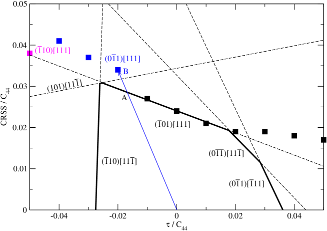
Figure 4.9: Loading path for compression at $\lambda=50^{\circ}$, $\chi=0$ superimposed on the ${\rm CRSS}-\tau$ dependence for the MRSSP $(\bar{1}01)$. The dashed lines are the critical lines calculated from the $\tau^{*}$ criterion with the inner envelope (solid line) corresponding to the yield polygon.

We have seen that the results of atomistic simulations, plotted in Fig. 3.9, correctly predict the $(0\bar{1}1)$ slip at negative shear stresses perpendicular to the slip direction that correspond to loading in compression. At the same time, the proposed $\tau^{*}$ criterion correctly predicts the onset of slip when $-0.02<\tau/C_{44}<+0.02$ for which the CRSS varies linearly with $\tau$. However, at large negative $\tau$, the atomistically calculated ${\rm CRSS}-\tau$ dependence is nonlinear, and the linear $\tau^{*}$ criterion does not reproduce the results of atomistic simulations sufficiently well. To illustrate this, we plot in Fig. 4.9 the loading path corresponding to compression along $\lambda=50^{\circ}$, $\chi=0$. From the $\tau^{*}$ criterion, slip occurs when the loading path reaches the yield polygon, particularly point A at which the $(\bar{1}01)[111]$ system becomes activated. However, using directly the atomistic results, one may argue that the slip occurs when the loading path reaches point B, which leads to the anomalous slip on the $(0\bar{1}1)[111]$ system. Ideally, both these predictions should give the same answer, and this agreement would certainly be achieved if $\tau^{*}$ were a nonlinear function of the applied stress. However, the nonlinear $\tau^{*}$ criterion would clearly introduce serious complications when predicting the ${\rm CRSS}-\chi$ and ${\rm CRSS}-\tau$ dependencies, and future finite-element simulations would become significantly more complicated and less efficient. Quoting Strogatz, (2003): ”No insight is gained if the model is as perplexing as the phenomena it’s supposed to describe”. The fact that the linear $\tau^{*}$ criterion does not directly predict the occurrence of the anomalous slip at negative $\tau$ is thus relevant only when dealing with microscopic details of the slip and does not affect the accuracy of the $\tau^{*}$ criterion in continuum analyses.

Table 4.3: The most operative slip systems predicted by the Schmid law and from the $\tau^{*}$ criterion, respectively, listed in the order of descending $\tau^{*}$. The Schmid factors and the values of $\tau^{*}$ are normalized by the values corresponding to the system with the highest $\tau^{*}$. The experimentally observed systems are written in bold.

a) $\lambda=50^{\circ}$, $\chi=+25^{\circ}$

order	ref. system	Schmid f.	$\tau^{*}$
1	$\bf(\bar{1}01)[\bar{1}\bar{1}\bar{1}]$	1.00	1.00
2	$\bf(\bar{1}10)[\bar{1}\bar{1}\bar{1}]$	0.90	0.97
3	$(101)[1\bar{1}\bar{1}]$	0.71	0.79
4	$(110)[1\bar{1}\bar{1}]$	0.57	0.71
5	$(101)[11\bar{1}]$	0.15	0.45
6	$(\bar{1}\bar{1}0)[\bar{1}1\bar{1}]$	0.06	0.41
7	$(\bar{1}10)[11\bar{1}]$	0.28	0.26
8	$(0\bar{1}\bar{1})[\bar{1}\bar{1}1]$	0.43	0.13
9	$(0\bar{1}1)[\bar{1}\bar{1}\bar{1}]$	0.10	0.10
$\vdots$	$\vdots$	$\vdots$	$\vdots$

b) $\lambda=50^{\circ}$, $\chi=0$ order ref. system Schmid f. $\tau^{*}$ 1 $\bf(\bar{1}01)[\bar{1}\bar{1}\bar{1}]$ 1.00 1.00 2 $\bf(101)[1\bar{1}\bar{1}]$ 0.90 0.96 3 $(\bar{1}10)[\bar{1}\bar{1}\bar{1}]$ 0.50 0.79 4 $(0\bar{1}1)[1\bar{1}\bar{1}]$ 0.65 0.69 5 $(0\bar{1}\bar{1})[\bar{1}\bar{1}1]$ 0.76 0.65 6 $(101)[11\bar{1}]$ 0.44 0.62 7 $\bf(0\bar{1}1)[\bar{1}\bar{1}\bar{1}]$ 0.50 0.60 $\vdots$ $\vdots$ $\vdots$ $\vdots$

c) $\lambda=50^{\circ}$, $\chi=-15^{\circ}$
order ref. system Schmid f. $\tau^{*}$ 1 $\bf(101)[1\bar{1}\bar{1}]$ 0.98 1.00 2 $\bf(\bar{1}01)[\bar{1}\bar{1}\bar{1}]$ 1.00 1.00 3 $(0\bar{1}1)[1\bar{1}\bar{1}]$ 0.89 0.87 4 $\bf(0\bar{1}1)[\bar{1}\bar{1}\bar{1}]$ 0.73 0.81 $\vdots$ $\vdots$ $\vdots$ $\vdots$

The discussion above holds also for the other loading direction, specifically $\lambda=50^{\circ}$, $\chi=-15^{\circ}$. Very briefly, the ratio $\eta$ of the two shear stresses resolved in the MRSSP at $\chi=-15^{\circ}$ is again negative, and thus the loading path in the ${\rm CRSS}-\tau$ projection passes between the atomistic data corresponding to slip on the $(\bar{1}01)$ and the $(0\bar{1}1)$ planes. Hence, the dislocation can again move on either of these two planes, which was, indeed, observed in experiments of Jeffcoat et al., (1976) for orientations corresponding to zero and negative $\chi$. Thus, the plastic deformation occurs via multiple slip of dislocations with Burgers vectors $1/2[111]$ and $1/2[\bar{1}11]$.

It is also important to check the degree of prominence of the most operative slip systems. This can be done either by comparing the Schmid factors or the $\tau^{*\alpha}$ values calculated for each system $\alpha$. For the three orientations of applied loading, Tab. 4.3 shows the Schmid factors and the $\tau^{*}$ values that are both normalized by the values corresponding to the system with the highest $\tau^{*}$. One can clearly see that the $\tau^{*}$ criterion predicts the increasing prominence of the $(0\bar{1}1)[\bar{1}\bar{1}\bar{1}]$ system for MRSSPs at zero and negative $\chi$. In particular, for $\chi=0$, this system is only the seventh most highly stressed one, but its activity increases at more negative $\chi$. For $\chi=-15^{\circ}$, this system is already the fourth most prominent one. A similar mechanism of slip, called hereafter “anomalous slip”, has been frequently encountered in low-temperature experiments on high purity single crystals of all bcc metals and thus seems to be a universal feature of slip of the group of VB and VIB metals.

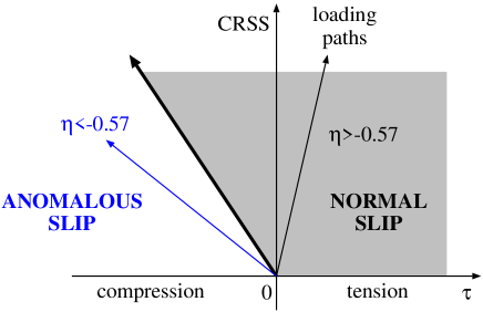
Figure 4.10: The two regions representing two different modes of slip.

Although the onset of anomalous slip under loading in compression is not directly predicted by the $\tau^{*}$ criterion, it can be directly predicted using the results of atomistic simulations performed at 0 K. The crucial observation is that the slip on the most highly stressed $(\bar{1}01)$ plane occurs when $\eta>-0.57$, where $\eta=\tau/\sigma$. In contrast, the slip on the anomalous $(0\bar{1}1)$ or $(\bar{1}10)$ plane takes place at larger negative $\tau$ or, more specifically, when $\eta<-0.57$. The orientations of loading paths leading to these two modes of slip are illustrated schematically in Fig. 4.10. The crossover value, $\eta\approx-0.57$, is independent of the orientation of the MRSSP and is thus a characteristic parameter of molybdenum. This suggests the possibility of finding a set of orientations of loading axes for which the atomistic results predict the onset of anomalous slip in compression. For any orientation of loading axis, this can be accomplished by resolving the shear stresses $\tau$ and $\sigma$ in the MRSSP and calculating their ratio $\eta$.

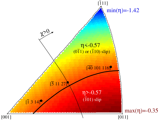
Figure 4.11: Distribution of the values of $\eta=\tau/\sigma$. The map is calculated for loading in compression in all possible directions inside the stereographic triangle. The solid line, $\eta\approx-0.57$, represents orientations for which the slip on the $(\bar{1}01)$ and either $(0\bar{1}1)$ or $(\bar{1}10)$ plane is equally likely.

Fig. 4.11 shows the distribution of the values of $\eta$ for loading in compression. As explained above, the orientations for which a $1/2[111]$ dislocation moves on the $(\bar{1}01)$ plane correspond to the region where $\eta>-0.57$, which is represented by the loading axes close to the $[011]$ corner of the triangle. However, for a large number of orientations closer to the $[001]-[\bar{1}11]$ edge, $\eta<-0.57$ and the slip proceeds on one of the low-stressed $\{110\}$ planes, as observed in atomistic simulations. All orientations of loading axes used in experiments of Jeffcoat et al., (1976) and plotted in Fig. 4.11 correspond to $\eta<-0.57$, which predicts the activation of slip on one of the two low-stressed $\{110\}$ planes.

4.7.4 Yield stress asymmetry in tension and compression

In order to investigate the plastic deformation of ultra-high purity single crystals of molybdenum under tension and compression, Seeger and Hollang, (2000) recently performed a series of experiments for three different orientations of applied loading and temperatures between $123~{}{\rm K}$ and $460~{}{\rm K}$. At high temperatures, approaching $460~{}{\rm K}$, the tensile and compressive yield stress of all crystals were practically the same. However, at temperatures close to $123~{}{\rm K}$ an interesting yield stress asymmetry arose for orientations $[\bar{1}49]$ and $[\bar{5}79]$ of tensile/compressive axes, which correspond to $\chi=0$ and $\chi=+21^{\circ}$, respectively, in that the yield stress in compression was appreciably higher than that obtained for the same orientation in tension.

In order to test whether our effective yield criterion is capable of predicting correctly this asymmetry between tension and compression, we will first introduce a stress differential

$$\Delta\sigma_{t,c}=\frac{\sigma_{t}-\sigma_{c}}{(\sigma_{t}+\sigma_{c})/2}\ ,$$ (4.8)

where $\sigma_{t}$ and $\sigma_{c}$ are the uniaxial yield stresses in tension and compression, respectively. For any orientation of applied loading, these yield stresses can be easily calculated from the tensorial form of the $\tau^{*}$ criterion (4.6). If one applies unit loading (+1 for tension, -1 for compression) along the given direction and calculates $\tau^{*\alpha}$ for each of the 24 slip systems from Tab. 4.2, the ratio $\tau_{cr}^{*}/\tau^{*\alpha}$ determines the magnitude of the uniaxial yield stress for each system $\alpha$. For a given loading axis, the actual yield stress that induces plastic flow in the crystal corresponds to the minimum value among the 24 possibilities, and the $\{110\}\langle{111}\rangle$ system corresponding to this value is the primary slip system that becomes operative first. By performing these calculations for all orientations in the stereographic triangle, one obtains a distribution of the stress differential (4.8) that is plotted in Fig. 4.12a. The effective yield criterion predicts that the yield stress in compression is larger than that in tension within a large area of the stereographic triangle. As the loading axis deviates from the center of the triangle towards the $[011]-[\bar{1}11]$ edge, $\sigma_{t}$ increases significantly and becomes equal to $\sigma_{c}$ for orientations along the solid line in Fig. 4.12a. For orientations closer to the $[011]$ corner of the triangle, $\sigma_{t}>\sigma_{c}$ and the sign of $\Delta\sigma_{t,c}$ becomes positive. The maximum asymmetry between the yield stress in tension and compression is reached for exactly the $[011]$ orientation in which case $\max(\Delta\sigma_{t,c})\approx+0.11$. For comparison, the minimum value of the stress differential, corresponding to the loading axis in the middle of the $[001]-[\bar{1}11]$ edge, is $\min(\Delta\sigma_{t,c})\approx-0.45$.

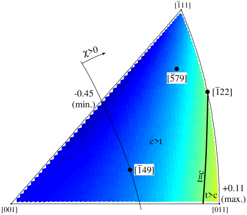
a) both shear stresses parallel and perpendicular to the slip direction considered
  
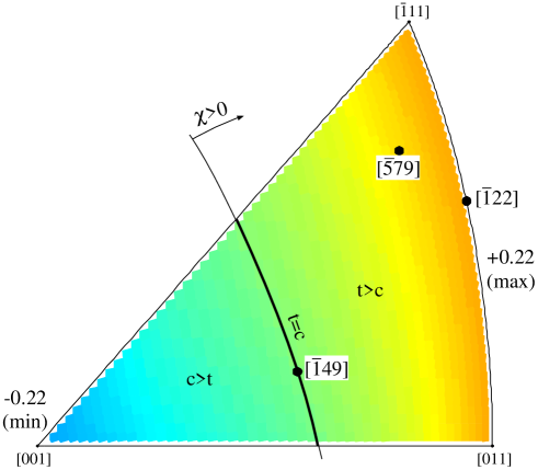
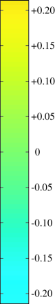
b) only shear stress parallel to the slip direction considered ($a_{2}=a_{3}=0$)

Figure 4.12: Maps of the stress differential $\Delta\sigma_{t,c}$ calculated from the $\tau^{*}$ criterion. Notice the antisymmetric character of $\Delta\sigma_{t,c}$ in b) but a more complex distribution in a).

If the twinning-antitwinning asymmetry were the only reason for the tension-compression asymmetry in molybdenum, the stress differential $\Delta\sigma_{t,c}$ would be antisymmetric with respect to $\chi$ and thus would necessarily vanish at $\chi=0$. This is shown in Fig. 4.12b, which corresponds to the restricted model of the $\tau^{*}$ criterion (4.1), i.e. when no shear stress perpendicular to the slip direction is considered. Clearly, the two distributions in Fig. 4.12 are very different. Therefore, the tension-compression yield stress asymmetry is not solely due to the twinning-antitwinning asymmetry. This discrepancy was identified already by Seeger and Hollang, (2000) and attributed to “a modification of the Peierls potential by stress components other than the resolved shear stress”. In the language of the non-associated plastic flow model, we identify this contribution as an effect of the shear stress perpendicular to the slip direction. It can be easily shown that the two non-glide stresses of the $\tau^{*}$ criterion that are proportional to $\tau$ do not vanish even for $\chi=0$, which thus gives rise to nonzero $\Delta\sigma_{t,c}$ for this orientation of the MRSSP.

In summary, the variation of the tension-compression yield stress asymmetry predicted by the $\tau^{*}$ criterion and plotted in Fig. 4.12a agrees qualitatively with the experimental observations of Seeger and Hollang, (2000). The comparison of the magnitudes of the stress differential is given in Tab. 4.4, where the values predicted from the $\tau^{*}$ criterion are taken from Fig. 4.12a and b. The reason why the agreement is only qualitative is that the experimental data correspond to 150 K, while the calculations using the $\tau^{*}$ criterion correspond to 0 K.

Table 4.4: Magnitudes of the stress differential calculated from the $\tau^{*}$ criterion and obtained from the experimental data of Seeger and Hollang, (2000) at the temperature 150 K. The theoretical data are obtained from the restricted and full forms of the $\tau^{*}$ criterion at 0 K, i.e. without and with shear stresses perpendicular to the slip direction.

	$\Delta\sigma_{t,c}$
	from $\tau^{*}$ (restricted)	from $\tau^{*}$ (full)	experiment
$[\bar{1}49],\chi=0$	0	-0.28	-0.06
$[\bar{5}79],\chi=+21^{\circ}$	+0.16	-0.21	-0.04
$[\bar{1}22],\chi=+29^{\circ}$	+0.21	0	+0.07

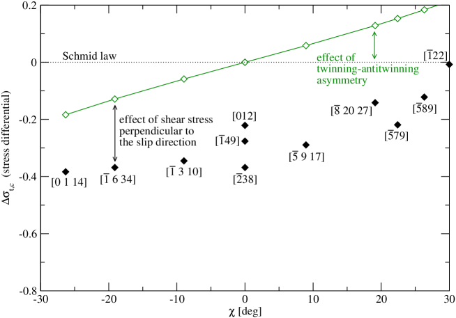
Figure 4.13: Variation of the stress differential (4.8) in molybdenum with the orientation of the MRSSP. The empty symbols are obtained from the restricted $\tau^{*}$ criterion (4.1) and the filled symbols from the full $\tau^{*}$ criterion (4.3).

To compare the contributions of the shear stresses parallel and perpendicular to the slip direction to the stress differential, we plot in Fig. 4.13 a variation of $\Delta\sigma_{t,c}$ with $\chi$. We include all the angles $\chi$ that correspond to the uniaxial loading axes in Fig. 3.6 as well as the three orientations in Tab. 4.4. For each of the loading axes, we first use the restricted form of the $\tau^{*}$ criterion to calculate the yield stresses $\sigma_{t}$, $\sigma_{c}$ which, in turn, determine the stress differential (4.8). This yields the data plotted in Fig. 4.13 with empty symbols that are further connected to highlight the antisymmetric character of $\Delta\sigma_{t,c}$ (see also Fig. 4.12b). It is important to emphasize, that the strength of the twinning-antitwinning asymmetry is proportional to the angle that this line makes with the prediction of the Schmid law. Subsequently, the same process is repeated using the full form of the $\tau^{*}$ criterion, which gives the data plotted with the filled symbols. The difference between the data obtained from the full and restricted models is obviously related to the effect of the shear stress perpendicular to the slip direction, which thus provides an important measure of the strength of these non-glide stresses. Clearly, the complex tension-compression asymmetry in molybdenum, shown in Fig. 4.12a, is a consequence of the combined effect of both the twinning-antitwinning asymmetry and the shear stress perpendicular to the slip direction.

4.7.5 Six degrees of freedom microstrain experiments

In recent years, the group of D. Lassila at Lawrence Livermore National Laboratory proposed and successfully executed a novel experimental technique in which five components of the elastic-plastic strain tensor, $\varepsilon_{ij}$, have been measured independently. The distinguishing feature of this technique is that the sample is essentially unconstrained with its bottom part able to slide freely on the substrate. This unconstrained motion prevents the rotation of the slip planes during loading. Knowing the total plastic strain tensor, obtained by eliminating the elastic contribution in $\varepsilon_{ij}$, the activities of 5 slip systems have been analyzed. Besides the identification of the dominant systems, this method also quantifies the degree of prominence of the slip on each of these systems, which is the key factor that can be used to correlate the predictions of the $\tau^{*}$ criterion with experiments.

Table 4.5: List of the slip systems whose activity was observed in the experiments of Lassila et al., (2003). The systems are sorted in order of descending Schmid factors. The values of $\tau^{*}$ are calculated for unit applied loading. The anomalous system is written in bold.

$\alpha$ (see Tab. 4.2)	slip system	Schmid factor	$\tau^{*}$
14	$(\bar{1}01)[\bar{1}\bar{1}\bar{1}]$	0.50	0.48
7	$(0\bar{1}\bar{1})[\bar{1}\bar{1}1]$	0.32	0.24
17	$(0\bar{1}1)[1\bar{1}\bar{1}]$	0.29	0.29
1	$\bf(0\bar{1}1)[\bar{1}\bar{1}\bar{1}]$	0.25	0.27
23	$(011)[\bar{1}1\bar{1}]$	0.22	0.16
10	$(10\bar{1})[1\bar{1}1]$	0.17	0.23

In the following, we concentrate on the experiment of Lassila et al., (2002, 2003) done on molybdenum under compression at room temperature, where the orientation of the loading axis is $[2\,\bar{9}\,\overline{20}]$. This orientation is characterized by angles $\lambda=45^{\circ}$, between the loading axis and the $[\bar{1}\bar{1}\bar{1}]$ slip direction, and $\chi=0$, between the MRSSP and the $(10\bar{1})$ reference plane. Because the loading in compression reverses the sense of shearing on the $(10\bar{1})$ plane, the most highly stressed system with positive Schmid factor is not $(10\bar{1})[\bar{1}\bar{1}\bar{1}]$ but, instead, its conjugate $(10\bar{1})[111]$. The list of the most prominent reference systems identified by Lassila et al., (2003) is given in Tab. 4.5, where the Miller indices are always written in such a way that each system can be found in Tab. 4.2. For example, instead of $(10\bar{1})[111]$, which does not appear in Tab. 4.2, we use an equivalent notation $(\bar{1}01)[\bar{1}\bar{1}\bar{1}]$, which corresponds to system 14.

Table 4.6: List of potentially active slip systems under loading in compression along $[2\,\bar{9}\,\overline{20}]$, orientation of the MRSSP of each system, and the stress ratio $\eta$ corresponding to positive shear stress $\sigma$ parallel to the slip direction. The anomalous system is written in bold.

ref. system	$\chi~{}[^{\circ}]$	$\tau/\sigma~{}(=\eta)$	predicted slip system	$\alpha$ in Tab. 4.5
$(\bar{1}0\bar{1})[\bar{1}11]$	14.0	-0.38	$(\bar{1}0\bar{1})[\bar{1}11]$, $(0\bar{1}1)[1\bar{1}\bar{1}]$	–, 17
$(0\bar{1}\bar{1})[\bar{1}\bar{1}1]$	12.3	-0.88	$(\bar{1}0\bar{1})[\bar{1}11]$, $(0\bar{1}1)[1\bar{1}\bar{1}]$	–, 17
$(10\bar{1})[1\bar{1}1]$	25.2	-2.45	$(0\bar{1}\bar{1})[\bar{1}\bar{1}1]$	7
$(\bar{1}01)[\bar{1}\bar{1}\bar{1}]$	0.0	-0.50	$(\bar{1}01)[\bar{1}\bar{1}\bar{1}]$, $\bf(0\bar{1}1)[\bar{1}\bar{1}\bar{1}]$	14, 1

For comparison, we list in Tab. 4.6 the four reference systems that can become operative because the orientation of their MRSSPs lies between $\pm 30^{\circ}$ from their reference planes, and the shear stress parallel to the slip direction is positive. The orientation of the MRSSP in each system is given by the angle $\chi$, and the ratio of the shear stress perpendicular to the shear stress parallel to the slip direction, resolved in the MRSSP, by the parameter $\eta$. Note, that all values of $\eta$ are negative, and, therefore, all loading paths in the ${\rm CRSS}-\tau$ projection of the corresponding MRSSP pass to negative $\tau$. The last two columns of the table give the slip systems predicted by the $\tau^{*}$ criterion and, if observed experimentally, the designation of this system referring to Tab. 4.5.

Figure 4.14: Projection of the critical lines (dashed lines) and the yield surface (solid polygon) in the ${\rm CRSS}-\tau$ graph corresponding to $\chi\approx+19^{\circ}$, which is close to the MRSSP of the reference system $(\bar{1}0\bar{1})[\bar{1}11]$ (see the first line in Tab. 4.6). The slope of the loading path is $\eta=-0.38$.

For example, the MRSSP of the $(\bar{1}0\bar{1})[\bar{1}11]$ system lies at $\chi=14^{\circ}$ and the stress ratio $\eta=-0.38$. This angle $\chi$ is close to $\chi\approx 19^{\circ}$ for which we have obtained earlier the ${\rm CRSS}-\tau$ dependence by means of atomistic simulations. These results were further generalized to real single crystals to arrive at Fig. 4.4c. However, since the reference system is now $(\bar{1}0\bar{1})[\bar{1}11]$ and not $(\bar{1}01)[111]$ as considered earlier, we need to transform the indices of the slip systems in Fig. 4.4c into this new basis. These transformations are explained in detail in Appendix B and provide the indices of the slip planes for the case when the $(\bar{1}0\bar{1})[\bar{1}11]$ is the reference system; see Fig. 4.14. Note, that the loading path plotted in this figure, corresponding to $\eta=-0.38$, first reaches the critical line for the $(\bar{1}0\bar{1})[\bar{1}11]$ system, which is thus predicted by the $\tau^{*}$ criterion to be the primary slip system. However, the loading path reaches the atomistic data between the points corresponding to slip on $(\bar{1}0\bar{1})$ and $(01\bar{1})$ planes. Consequently, two of the most operative slip systems predicted by the $\tau^{*}$ criterion (and atomistic results) are $(\bar{1}0\bar{1})[\bar{1}11]$ and $(01\bar{1})[\bar{1}11]$. The latter system can be equivalently written as $(0\bar{1}1)[1\bar{1}\bar{1}]$, which is identical to the experimentally observed slip system 17 with the Schmid factor 0.29 (see Tab. 4.5).

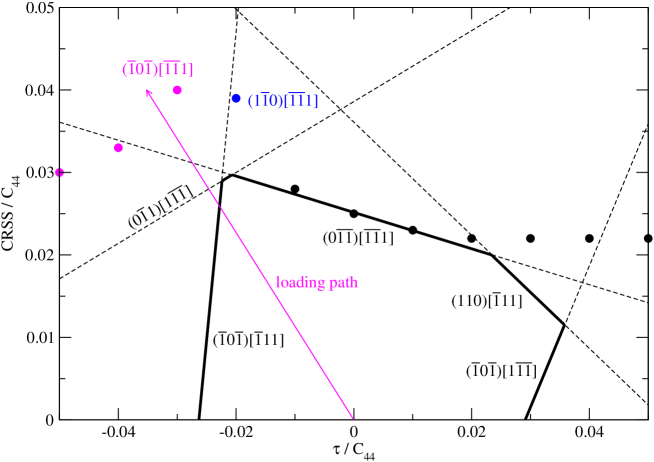
Figure 4.15: Projection of the critical lines (dashed lines) and the yield surface (solid polygon) in the ${\rm CRSS}-\tau$ graph corresponding to $\chi\approx+9^{\circ}$, which is close to the MRSSP of the reference system $(0\bar{1}\bar{1})[\bar{1}\bar{1}1]$ (see the second line in Tab. 4.6). The slope of the loading path is $\eta=-0.88$.

The next potentially operative slip system listed in Tab. 4.6 is $(0\bar{1}\bar{1})[\bar{1}\bar{1}1]$ with MRSSP at $\chi=12.3^{\circ}$ and $\eta=-0.88$. In Fig. 4.15, we plot the ${\rm CRSS}-\tau$ data for $\chi\approx 9^{\circ}$ calculated from the atomistic simulations together with the critical lines obtained from the $\tau^{*}$ criterion for molybdenum. The loading path plotted in this figure, corresponding to $\eta=-0.88$, first reaches the $(\bar{1}0\bar{1})[\bar{1}11]$ system, which thus becomes the predicted primary slip system. Furthermore, since the CRSS for slip on the secondary system, $(0\bar{1}1)[1\bar{1}\bar{1}]$, is virtually identical, one may expect that the two systems will operate simultaneously. This secondary system coincides with that obtained by cross-slip from the $(\bar{1}0\bar{1})[\bar{1}11]$ system above and is indeed one of the operative systems in the experiments of Lassila et al., (2003).

The same analysis for the remaining two slip systems in Tab. 4.6 and their comparison with experimental observations of Lassila et al., (2003) is summarized in the last two columns of this table. For the last system listed, $(\bar{1}01)[\bar{1}\bar{1}\bar{1}]$, the loading path given by $\eta=-0.5$ is close to that for compression along $[\bar{2}38]$ (Fig. 3.9a), and, therefore, the slip on the same slip plane, at $\psi=+60^{\circ}$, should be anticipated. The corresponding index of the slip plane is found from Fig. 4.1 to be $(0\bar{1}1)$. Because the Schmid factor for the system $(0\bar{1}1)[\bar{1}\bar{1}\bar{1}]$ is only the fourth highest one (see Tab. 4.5), this gives rise to the anomalous slip whose activity is also observed in the experiments of Lassila et al., (2003).

From the analysis given above, one can observe that the $\tau^{*}$ criterion predicts the activation of four out of six slip systems whose operation is observed experimentally at the room temperature. Although the six degrees of freedom experiments were originally designed to validate the results of large-scale dislocation dynamics experiments (Lassila et al.,, 2002), the agreement with the $\tau^{*}$ criterion is a strong indication that macroscopic plastic flow of bcc molybdenum can be accurately obtained using simple linear yield criteria based on single-dislocation studies.

4.8 Origin of the $(0\bar{1}1)$ slip in tension

Under tensile loading, the shear stress perpendicular to the slip direction is always positive (i.e. $\eta>0$), and the atomistic data predict that a $1/2[111]$ screw dislocation will move on the $(\bar{1}01)$ plane. This is in agreement with many experimental studies, some of which have been cited earlier in this chapter (Lau and Dorn,, 1970; Aono et al.,, 1983). In principle, the operation of the $(0\bar{1}1)[111]$ system is possible even in tension and arises naturally from the proposed $\tau^{*}$ criterion (4.6).

Let us look at Fig. 4.16 showing a set of critical lines calculated from the $\tau^{*}$ criterion and projected in the ${\rm CRSS}-\tau$ graph of the MRSSP $(\bar{5}\bar{4}9)$ corresponding to $\chi=-26^{\circ}$. Consider uniaxial loading in tension for which the loading path emanates from the origin and passes to the region of positive $\tau$. When this loading path reaches the inner envelope of the critical lines at its corner, many slip systems become spontaneously operative. One of these systems is $(0\bar{1}1)[111]$, whose critical line should ideally interpolate the atomistic data corresponding to slip on the $(0\bar{1}1)$ plane at negative $\tau$. It is important to emphasize that this must not be confused with the anomalous slip, because $(0\bar{1}1)[111]$ is now one of the dominant slip systems with a large Schmid factor. Consequently, the observation of the $(0\bar{1}1)$ slip in tension at $\chi\rightarrow-30^{\circ}$ and in compression corresponds to two different modes of slip.

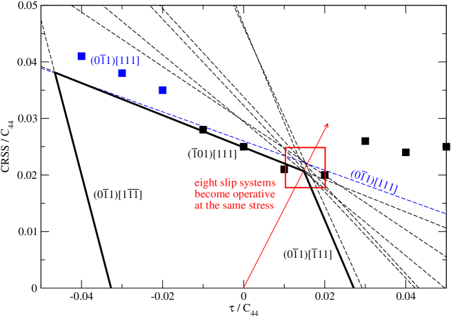
Figure 4.16: Onset of slip on the $(0\bar{1}1)[111]$ system under tension. For the loading path depicted, many slip systems become operative simultaneously. The calculated Schmid factors and the values of $\tau^{*}$ are listed in Tab. 4.7.

To support the above conclusions, we show in Tab. 4.7 the complete list of all slip systems that can be activated under loading in tension along $[0\,1\,14]$, corresponding to $\chi=-26^{\circ}$. The loading path for this orientation agrees closely with that plotted in Fig. 4.16. The observation that the eight systems will be actived simultaneously is equivalent to saying that all these systems have similarly high values of $\tau^{*}$. This is confirmed by looking at the actual values of both Schmid stresses and $\tau^{*}$ given in Tab. 4.7. Since $\tau^{*}$ for all eight systems is within 91% of that for the most-highly stressed $(\bar{1}01)[111]$ system, they will in reality act concomitantly, which will result in a burst of slip activity at the stress for which the loading reaches the corner of the inner polygon in Fig. 4.16.

Table 4.7: The list of all slip systems that can become operative under loading in tension along $[0\,1\,14]$ for which the corresponding MRSSP is at $\chi\approx-26^{\circ}$ and $\eta=0.64$. The Schmid stresses and the values of $\tau^{*}$ are normalized by the values obtained for the primary slip system, $(\bar{1}01)[111]$.

slip system	Schmid stress	$\tau^{*}$
$(\bar{1}01)[111]$	1.00	1.00
$(101)[\bar{1}11]$	1.00	1.00
$(011)[1\bar{1}1]$	0.93	0.96
$(0\bar{1}\bar{1})[11\bar{1}]$	0.93	0.96
$(0\bar{1}1)[\bar{1}11]$	0.93	0.94
$(0\bar{1}1)[111]$	0.93	0.94
$(101)[\bar{1}\bar{1}1]$	0.87	0.91
$(10\bar{1})[\bar{1}1\bar{1}]$	0.87	0.91

The fact that the $(0\bar{1}1)[111]$ system increases its prominence as $\chi\rightarrow-30^{\circ}$ implies that, for these orientations of tensile loading, $1/2[111]$ dislocations can equally well glide on both $(\bar{1}01)$ and $(0\bar{1}1)$ planes. This gives rise to the zig-zag slip on these two planes that manifests itself as a macroscopic slip on one of the intermediate planes. In particular, macroscopic slip on the $(\bar{1}\bar{1}2)$ plane emerges if the elementary steps on these two planes are of equal size. This $\{112\}$ slip was indeed observed in tensile experiments of Lau and Dorn, (1970) for orientation $[\bar{1}17]$, corresponding to $\chi=-16^{\circ}$, denoted thereafter as A. For all other orientations at $\chi>-16^{\circ}$, the glide of the dislocation proceeded entirely on the most highly stressed $(\bar{1}01)$ plane. Interestingly, Aono et al., (1989) report the “anomalous” slip in tension for orientations $\chi<+16^{\circ}$ and temperature 77 K. However, slip on the $(0\bar{1}1)$ plane was dominant only to about 1% of plastic strain and became completely suppressed at higher strains, where the $(\bar{1}01)[111]$ system governed the plastic flow. According to Aono et al., (1983), the $(0\bar{1}1)$ slip in tension completely vanishes at 4.2 K, and the dislocation moves on the $(\bar{1}01)$ plane for any orientation of the MRSSP.

The main result of the analysis presented above is that the glide of a $1/2[111]$ dislocation on the $(0\bar{1}1)$ plane is indeed possible and is correctly predicted by the $\tau^{*}$ criterion for large negative angles $\chi$. However, this is not to be confused with the anomalous slip because the Schmid stress for the $(0\bar{1}1)[111]$ system is comparable to that of the primary slip system, $(\bar{1}01)[111]$; see Tab. 4.7.

Chapter 5 Thermally activated plastic flow in molybdenum

Once you eliminate the impossible, whatever remains,

no matter how improbable, must be the truth.

Sherlock Holmes

We will now proceed to formulate a mesoscopic phenomenological theory of thermally activated motion of screw dislocations that is based on the results of atomistic calculations. The link between the microscopic behavior of screw dislocations and the mesoscale will be conveniently traversed by the effective yield criterion that we constructed in Chapter 4 and that was shown to reproduce correctly experimental measurements.

5.1 Thermodynamics of dislocation glide

In this development we consider that the motion of screw dislocations in bcc crystals is driven by the applied stress and opposed by the lattice friction. At 0 K a screw dislocation can be regarded as a straight line that assumes a position at which the Peach-Koehler force exerted on the dislocation by the applied stress and the restoring force due to the lattice friction balance each other. In order to move the dislocation, the applied stress must be large enough to transform the dislocation into a glissile configuration. At finite temperatures a saddle-point configuration is attained at a stress lower than that needed for the dislocation glide at 0 K, because a part of the energy needed to reach this configuration is supplied by thermal fluctuations. This is the reason why the stress needed to sustain a certain rate of dislocation motion decreases with increasing temperature. Such process leads to thermally activated dislocation glide.

The Gibbs free energy of activation for the dislocation glide depends crucially on the choice of the thermodynamic variables that remain constant during the activation. Following Schoeck, (1965) and Hirth and Nix, (1969), we will consider that temperature $T$, pressure $p$, applied stress $\sigma$, and surface energy $\gamma$ remain constant. The elementary change of the Gibbs free energy during the activation can then be written as

$${\rm d}G={\rm d}U-T{\rm d}S+p{\rm d}V-\sigma{\rm d}\varepsilon-\gamma{\rm d}A\ ,$$ (5.1)

where $U,S,V,\sigma,\varepsilon,\gamma,A$ are the internal energy, entropy, volume, applied stress, strain, surface energy, and surface area of the system, respectively. The change of volume and surface area during the activation is usually small and can thus be safely neglected. Defining the change of enthalpy as ${\rm d}H={\rm d}U-\sigma{\rm d}\varepsilon$, one directly arrives at an equality ${\rm d}G={\rm d}H-T{\rm d}S$. The total change of the Gibbs free energy during the activation can then be obtained directly by integrating the last equation between the configuration of the dislocation and the saddle-point, which yields the well-known formula

$$\Delta{G}=\Delta{H}-T\Delta{S}\ .$$ (5.2)

According to the transition state theory (Caillard and Martin,, 2003; Kocks et al.,, 1975), the rate of arriving at the saddle-point follows an Arrhenius law

$$\nu=\nu_{0}\exp\left(-\frac{\Delta{G}}{kT}\right)\equiv\nu_{0}^{*}\exp\left(-\frac{\Delta{H}}{kT}\right)\ ,$$ (5.3)

where $\nu_{0}$ is the frequency of unconstrained vibrations, and $\nu_{0}^{*}=\nu_{0}\exp(\Delta S/k)$ is an effective vibrational frequency that accounts for the change in entropy during the activation. Within the framework of the rate theory of Vineyard, (1957), the effective frequency $\nu_{0}^{*}$, involving the entropy $\Delta{S}$, is the ratio of the product of $N$ normal frequencies, $\nu_{j}$, of the system at the starting point of the transition to the product of $N-1$ normal frequencies of the system at the saddle-point configuration, $\nu_{j}^{\prime}$, so that

$$\nu_{0}^{*}=\prod_{j=1}^{N}\nu_{j}\left/\ \prod_{j=1}^{N-1}\nu_{j}^{\prime}\right.\ .$$ (5.4)

Celli et al., (1963) suggested the separation of these vibrational modes into two mutually noninteracting classes: dislocation modes and crystal modes. The crystal modes in the starting and the saddle-point configurations are assumed to be identical and to cancel each other in Eq. 5.4. Then, in order to apply Vineyard’s formula, it is sufficient to calculate the ratio of the product of the dislocation modes in the starting configuration to that in the saddle-point activated state. This product was explicitly evaluated for square-shaped activation barriers by Celli et al., (1963). In general, the usual approach is to consider in the starting configuration only the frequency of vibration in the direction of motion, i.e. the so-called attack frequency. This frequency can be approximated as $\nu_{D}(l/b)$, where $\nu_{D}$ is the Debye frequency, $l$ the dislocation length involved in the activation process, and $b$ the magnitude of the Burgers vector. Since this frequency is missing in the activated state, $\nu_{0}^{*}$ is written as $\nu_{D}(l/b)$. The velocity of the dislocation can then be written as $v_{D}=a_{0}\nu_{0}^{*}\exp(-\Delta{H}(\sigma)/kT)$, where $a_{0}$ is the distance traversed during the activation event. Assuming that only one slip system operates, the strain rate can be written as $\dot{\gamma}=\rho_{m}bv_{D}$ or, equivalently, as

$$\dot{\gamma}=\dot{\gamma}_{0}\exp\left(-\frac{\Delta H(\sigma)}{kT}\right)\ ,$$ (5.5)

with the pre-exponential factor $\dot{\gamma}_{0}=\rho_{m}a_{0}b\nu_{0}^{*}$ (Kocks et al.,, 1975; Caillard and Martin,, 2003). Here, $\rho_{m}$ is the density of mobile dislocations actively participating in the gliding process, and $b$ the magnitude of their Burgers vector. The stress dependence of $\dot{\gamma}_{0}$ is usually neglected, since it is much weaker than the exponential dependence on stress via $\Delta{H}(\sigma)$, and, for similar reasons, one usually makes the assumption that the mobile dislocation density, $\rho_{m}$, is a constant. The determination of the stress dependence of the activation enthalpy, $\Delta{H}(\sigma)$, based on the results of atomistic studies, is the main topic of this chapter. For the sake of brevity, we will further drop the symbol $\Delta$ in the designation of the activation enthalpy.

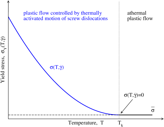
Figure 5.1: Schematic illustration of the temperature dependence of the yield stress in bcc metals.

At high temperatures, the yield stress of bcc metals is only weakly dependent on temperature via the temperature dependence of elastic moduli and can be approximated by a constant athermal stress $\bar{\sigma}$. On the other hand, at low temperatures, the plastic flow is controlled by the thermally activated motion of screw dislocations, and the yield stress is a strong function of both temperature and plastic strain rate. One can, therefore, write the actual yield stress as a sum of two terms,

$$\sigma_{Y}(T,\dot{\gamma})=\sigma(T,\dot{\gamma})+\bar{\sigma}\ ,$$ (5.6)

where $\sigma(T,\dot{\gamma})$ is the thermal component of the yield stress that depends on both temperature $T$ and plastic strain rate $\dot{\gamma}$. $\sigma(T,\dot{\gamma})$ vanishes at the temperature $T_{k}$, where the yield stress approaches its athermal value, $\bar{\sigma}$. Below $T_{k}$, the thermal component $\sigma(T,\dot{\gamma})$ gradually increases and reaches its maximum at $0~{}{\rm K}$ (see Fig. 5.1).

In the following, we will be concerned with the thermally activated motion of screw dislocations at temperatures below $T_{k}$. This will provide us with the variation of the thermal component of the yield stress, $\sigma(T,\dot{\gamma})$, which can be compared with the thermal component of the yield stress obtained from experiments by subtracting from the measured yield stress the constant athermal stress $\bar{\sigma}$.

5.2 Activation enthalpy of formation of pairs of kinks

It is generally accepted that at finite temperatures screw dislocations in bcc metals overcome the Peierls barriers by nucleating pairs of kinks that subsequently migrate, which leads to the glide of the dislocation in the direction of the kink formation. As discussed in the preceding chapters, the dislocation core changes under the influence of the applied stress, and this is considered phenomenologically as shifting the dislocation as a straight line toward the top of the barrier. In this work, the shape of the Peierls barrier is considered to be a function of non-glide stresses, while the work on shifting the dislocation toward the top of this barrier is done purely by the applied Schmid stress.

At low temperatures and high stresses the dislocation core is almost transformed to the glissile form and, phenomenologically, the dislocation has been moved by stress almost to the top of the barrier. Hence, a relatively small thermal energy is needed to overcome the barrier. In this regime, the activated state consists of a continuous “bow-out” developed on otherwise straight screw dislocation (Dorn and Rajnak,, 1964; Duesbery,, 1989), as shown in the right panel of Fig. 5.2. On the other hand, at high temperatures (left panel in Fig. 5.2), thermal fluctuations are large and only a small stress is needed to move the dislocation through the crystal. In this case, the dislocation core is only slightly distorted, which in the phenomenological analysis means that the dislocation moves as a straight line only a short distance. Thermal fluctuations then help to nucleate a pair of kinks that attract each other elastically via their long-range strain fields (Seeger,, 1956), and the saddle-point configuration corresponds to two well-separated kinks at the distance for which the attraction between the kinks is compensated by the force exerted on them by the applied Schmid stress.

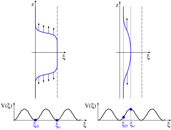
Figure 5.2: Schematic illustration of the nucleation of a pair of kinks at low stresses and high temperatures (left panel) and of the critical bow-out at high stresses and low temperatures (right panel). $\xi$ designates the activation path and $V(\xi)$ the Peierls barrier along this path.

Dislocations in crystalline materials experience lattice friction that varies periodically with the position of the dislocation in the crystal. At finite temperatures, the Peierls barrier is overcome partly due to the work done with the aid of thermal fluctuations and the work done by the applied Schmid stress during the activation process. In contrast, the activation barrier is the fraction of the Peierls barrier that is left after subtracting the work done by the Schmid stress when shifting the dislocation up on the barrier. The construction of the Peierls barrier will be explained in detail in Section 5.4.

5.2.1 Energy of an isolated kink

The energy of a single isolated kink was first derived by Seeger, (1956) in an attempt to explain the low-temperature internal friction peak in polycrystals. In his work, the saddle-point energy corresponds to a pair of two fully developed kinks, interacting with each other, at the separation for which the mutual attraction of the kinks is compensated by the applied stress. These calculations were later revisited by Dorn and Rajnak, (1964) who successfully demonstrated that the kink-pair formation model can be utilized to explain the low-temperature increase of the yield stress in bcc metals. In contrast to the model of Seeger, (1956), the saddle-point configuration is represented by a continuous bow-out on an otherwise straight screw dislocation, which is attained before a pair of two fully developed interacting kinks is formed.

In the original theory (Seeger,, 1956; Dorn and Rajnak,, 1964), the Peierls potential was written as a periodic function of the position of the dislocation in a well-defined slip plane. The only component of the stress tensor considered was the shear stress in the slip plane acting parallel to the Burgers vector. Although widely observed in experiments on molybdenum and other bcc metals, no twinning-antitwinning asymmetry was predicted from these early models. More recently, Edagawa et al., (1997) suggested that the Peierls potential should be a two-dimensional function of the position of the intersection of the dislocation with the $\{111\}$ plane that is perpendicular to the dislocation line. The Peierls barrier was identified with the profile of the two-dimensional Peierls potential along a curved transition path between two adjacent low-energy sites in the $\{111\}$ plane, and was considered to be a function of the shear stress parallel to the slip direction. This model captured not only the twinning-antitwinning asymmetry in molybdenum but also the stress dependence of the activation enthalpy and thus the trend of the temperature dependence of the yield stress.

If the functional form of the Peierls potential is given as a function $V(x,y)$ defined in the $\{111\}$ plane, the energy of a single kink can be determined as

$$H_{k}=\int_{-\infty}^{\infty}\left[V(x,y)\,{\rm d}s-V_{0}\,{\rm d}z\right]\ ,$$ (5.7)

where ${\rm d}s$ is an elementary segment along the kinked dislocation, $V_{0}$ the magnitude of the potential at the bottom of the Peierls valley, and ${\rm d}z$ an element along the $z$ axis that is parallel to the straight dislocation. In this formulation, $V$ can be regarded as the energy per unit length of the dislocation found at a particular position in the Peierls potential valley. The kink energy $H_{k}$, given by equation (5.7), is defined as the difference between the line energy of the kinked dislocation and the line energy of a straight dislocation at the bottom of the Peierls valley. Because the dislocation is now a three-dimensional curve, ${\rm d}s=\sqrt{({\rm d}x)^{2}+({\rm d}y)^{2}+({\rm d}z)^{2}}$ and (5.7) then reads

$$H_{k}=\int_{-\infty}^{\infty}\left[V(x,y)\sqrt{1+\left(\frac{{\rm d}x}{{\rm d}z}\right)^{2}+\left(\frac{{\rm d}y}{{\rm d}z}\right)^{2}}-V_{0}\right]{\rm d}z\ .$$ (5.8)

From the 0 K atomistic simulations, we know that screw dislocations in molybdenum move on $\{110\}$ planes by discrete jumps between two adjacent minima of the Peierls potential $V(x,y)$. The transition path between these minima is always a continuous curve and corresponds to the minimum energy path (MEP). When forming the kink, the dislocation bows-out along the MEP specified by a curve $\xi(z)$. The elements ${\rm d}x$ and ${\rm d}y$, defined in the $\{111\}$ plane perpendicular to the dislocation line, can be written as ${\rm d}x={\rm d}\xi\cos\theta$ and ${\rm d}y={\rm d}\xi\sin\theta$, where $\theta$ is at any point along the MEP the angle between the tangent of the MEP and the $x$ axis. Substituting these expressions into (5.8) and using the identity $\sin^{2}\theta+\cos^{2}\theta=1$ reduces the expression for the kink energy to:

$$H_{k}=\int_{-\infty}^{\infty}\left[V(\xi)\sqrt{1+\left(\xi^{\prime}(z)\right)^{2}}-V_{0}\right]{\rm d}z\ ,$$ (5.9)

where we replaced $V(x,y)$ by $V(\xi)$, profile of the Peierls potential along the MEP, and wrote $\xi^{\prime}(z)={\rm d}\xi/{\rm d}z$. Following Dorn and Rajnak, (1964), the stationary solution of Eq. 5.9, corresponding to the maximum of $H_{k}$, is given by the Euler-Lagrange equation

$$\left(\frac{\partial}{\partial{\xi}}-\frac{{\rm d}missing}{{\rm d}z}\frac{\partial}{\partial\xi^{\prime}(z)}\right)\left[V(\xi)\sqrt{1+\left(\xi^{\prime}(z)\right)^{2}}\right]=0\ ,$$ (5.10)

which reads, after differentiation,

$$\frac{{\rm d}missing}{{\rm d}\xi}\left(\frac{V(\xi)}{\sqrt{1+\left(\xi^{\prime}(z)\right)^{2}}}\right)=0\ .$$ (5.11)

This equation can be integrated once to get the slope of the dislocation line with a kink,

$$\xi^{\prime}(z)=\pm\sqrt{\left(\frac{V(\xi)}{C}\right)^{2}-1}\ ,$$ (5.12)

where $C$ is an integration constant. Assume that one end of the dislocation lies in the Peierls valley determined by $\xi=0$ and the other in the neighboring valley at $\xi_{max}$ (measured along the curved MEP). The slope of the dislocation at $\xi=0$ and $\xi_{max}$ then vanishes and this suggests two boundary conditions: (i) $\xi=0\Rightarrow z\rightarrow-\infty$, $\xi^{\prime}(-\infty)=0$ and $V(0)=V_{0}$, and (ii) $\xi=\xi_{max}\Rightarrow z\rightarrow+\infty$, $\xi^{\prime}(+\infty)=0$ and $V(\xi_{max})=V_{0}$. In the case of an opposite kink, one has to interchange the plus and minus signs. Because the slope $\xi^{\prime}(z)$ of the dislocation is zero at $\xi=0$ and $\xi_{max}$, where the corresponding height of the Peierls potential is $V_{0}$, Eq. 5.12 gives the magnitude of the integration constant, $C=V_{0}$. Finally, substituting Eq. 5.12 together with the value of $C$ into Eq. 5.9 gives the energy of an isolated kink,

$$H_{k}=V_{0}\int_{0}^{\xi_{max}}\sqrt{\left(\frac{V(\xi)}{V_{0}}\right)^{2}-1}\ {\rm d}\xi\ ,$$ (5.13)

where we changed the integration variable by substituting ${\rm d}z$ as a function of ${\rm d}\xi$ from (5.12). In Eq. 5.13, the kink energy is determined as a path integral between two potential minima calculated along the curved MEP.

5.2.2 High stresses: dislocation bow-out

At a nonzero stress, the dislocation is moved away from the bottom of the Peierls valley as a straight line by the action of the applied Schmid stress $\sigma$. The position at which the force ${\rm d}V/{\rm d}\xi$, originating from the Peierls potential, is equal to the Peach-Koehler force $\sigma b$, induced by the applied stress, will be denoted as $\xi_{0}$. At high stresses, the dislocation bows-out toward the top of the Peierls barrier and the activated state corresponds to the maximum of the enthalpy. Starting with Eq. 5.9, the enthalpy associated with the dislocation bowing-out along the MEP is

$$H_{b}=\int_{-\infty}^{\infty}\left[V(\xi)\sqrt{1+\left(\xi^{\prime}(z)\right)^{2}}-V(\xi_{0})-\sigma b(\xi-\xi_{0})\right]{\rm d}z\ .$$ (5.14)

Here, the first term in the integrand is the line energy of the curved dislocation bowed-out along the MEP, and the last two terms are the line energy of a straight dislocation at $\xi_{0}$ and the work done by the stress $\sigma$ when displacing the dislocation from $\xi_{0}$ to $\xi$. As in the case of zero stress, we are looking for a stationary shape of the dislocation that is given by the Euler-Lagrange equation

$$\left(\frac{\partial}{\partial{\xi}}-\frac{{\rm d}missing}{{\rm d}z}\frac{\partial}{\partial\xi^{\prime}(z)}\right)\left[V(\xi)\sqrt{1+\left(\xi^{\prime}(z)\right)^{2}}-V(\xi_{0})-\sigma b(\xi-\xi_{0})\right]=0\ .$$ (5.15)

Performing the indicated differentiation, this immediately simplifies to

$$\sigma b=\frac{{\rm d}missing}{{\rm d}\xi}\left(\frac{V(\xi)}{\sqrt{1+\left(\xi^{\prime}(z)\right)^{2}}}\right)\ .$$ (5.16)

Integrating and solving for the slope $\xi^{\prime}(z)$ gives

$$\xi^{\prime}(z)=\pm\sqrt{\left(\frac{V(\xi)}{\sigma b\xi+C}\right)^{2}-1}\ ,$$ (5.17)

where $C$ is an integration constant that can be determined by demanding that the slope of the dislocation at $z\rightarrow\pm\infty$ and $\xi\rightarrow\xi_{0}$ remains zero. These boundary conditions yield $C=V(\xi_{0})-\sigma b\xi_{0}$, which can be substituted back into (5.17) to obtain the slope of the dislocation in the activated state:

$$\xi^{\prime}(z)=\pm\sqrt{\left(\frac{V(\xi)}{\sigma b(\xi-\xi_{0})+V(\xi_{0})}\right)^{2}-1}\ .$$ (5.18)

Each sign in this equation defines the slope in one-half of the bowed dislocation that meet at $z=0$. The stationary magnitude of the bow-out, denoted hereafter as $\xi_{m}$, is determined from the condition $\xi^{\prime}=0$ for $z=0$. It then follows from (5.18) that $\xi_{m}$ is determined by the relation

$$V(\xi_{m})-V(\xi_{0})=\sigma b(\xi_{m}-\xi_{0})\ .$$ (5.19)

One solution is $\xi_{m}=\xi_{0}$ (Fig. 5.3), and this corresponds to the straight dislocation at $\xi_{0}$ when $H_{b}=0$, which is the minimum value of the enthalpy given by Eq. 5.14. The second solution, $\xi_{m}=\xi_{c}$ (Fig. 5.3), defines the segment of the dislocation in the critical configuration for which the activation enthalpy reaches a maximum and the bow-out represents a saddle-point configuration. No stationary solution for the bow-out exists for $\xi_{0}<\xi_{m}<\xi_{c}$, since in this case the two kinks of the bow-out annihilate each other. Similarly, no stationary solution exists for $\xi_{m}>\xi_{c}$, because in this case the two kinks are driven apart by the applied stress.

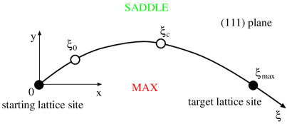
Figure 5.3: Schematic depiction of a curved transition coordinate $\xi$ for a dislocation moving between two minimum energy sites (filled circles). SADDLE and MAX designate a saddle-point and a maximum of the Peierls potential, respectively. At zero applied stress the kink develops from $0$ to $\xi_{max}$, whereas at finite stresses the kink only extends from $\xi_{0}$ to $\xi_{c}$.

The enthalpy of nucleation of the critical bow-out on the dislocation line at high stresses is obtained by substituting (5.18) into (5.14) that gives

$$H_{b}=2\int_{\xi_{0}}^{\xi_{c}}\sqrt{\left[V(\xi)\right]^{2}-\left[\sigma b(\xi-\xi_{0})+V(\xi_{0})\right]^{2}}\ {\rm d}\xi\ ,$$ (5.20)

where we again changed the integration variable by realizing that ${\rm d}z$ can be written as a function of ${\rm d}\xi$ by inverting the slope (5.18). The factor of 2 ahead of the integral arises because the integrand is a double-valued function of $\xi$ that is even about $z=0$ and, therefore, the integration gives only one-half of the activation enthalpy. The activation enthalpy (5.20) is illustrated in Fig. 5.4 as an area bounded by the Peierls barrier, $V(\xi)$, and the line with the slope $\sigma b$. It is important to realize that $V(\xi)$ is the line energy of the dislocation at position $\xi$ along the MEP, which can never be lower than $V_{0}$, the line energy of the dislocation lying at the bottom of the Peierls valley. This requires that the zero of energy, i.e. the minimum of $V(x,y)$, coincides with $V_{0}$. In the following, we write $V_{0}=p\mu b^{2}$, where $\mu$ is the $\langle{111}\rangle$ shear modulus, and $p$ a constant whose magnitude will be determined in Section 5.2.4.

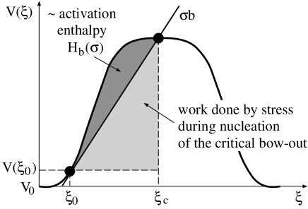
Figure 5.4: Graphical interpretation of Eq. 5.20 in which the activation enthalpy is calculated as a function of the applied stress $\sigma$.

The activation enthalpy (5.20) ceases to be applicable at low stresses (high temperatures), where an alternative saddle-point configuration, consisting of two fully developed kinks spanning from one minimum of the Peierls potential to the next, becomes energetically more favorable. The saddle-point configuration then corresponds to the separation of these kinks at which their attraction is compensated by the force exerted on them by the Schmid stress $\sigma$ that pushes them apart. The derivation of the activation enthalpy in this low-stress regime will concern us in the following section. In the limit of zero stress, one can easily see that $H_{b}\rightarrow 2H_{k}$, and the activation enthalpy coincides with the energy of two isolated (non-interacting) kinks.

Based on the stress dependence of the activation enthalpy given by Eq. 5.20, one can calculate the so-called activation volume, $V_{b}=-\partial{H_{b}}/\partial{\sigma}$, which can be directly measured in experiments (Conrad and Hayes,, 1963). The explicit forms of the activation volumes for a limited class of simple one-dimensional Peierls potentials can be found in Caillard and Martin, (2003).

5.2.3 Low stresses: elastic interaction of fully developed kinks

At low applied stresses, i.e. high temperatures, the shape of the dislocation in the activated configuration is represented by a pair of kinks that interact elastically via the attractive Eshelby potential $\mu a_{0}^{2}b^{2}/8\pi\Delta{z}$ (Caillard and Martin,, 2003), where $a_{0}$ is the height of the kinks or, equivalently, the distance between two neighboring Peierls valleys in the slip plane, and $\Delta{z}$ their separation. This attractive interaction is opposed by the applied shear stress $\sigma$ during the nucleation which does work equal to $\sigma a_{0}b\Delta{z}$. The enthalpy of nucleation of a pair of interacting kinks in the low-stress regime, $H_{kp}$, is then determined by competition between the attractive elastic interaction and the work done on displacing the two kinks a distance $\Delta{z}$ apart,

$$H_{kp}=2H_{k}-\frac{\mu a_{0}^{2}b^{2}}{8\pi\Delta{z}}-\sigma a_{0}b\Delta{z}\ ,$$ (5.21)

where $2H_{k}$ is the energy of two isolated kinks. At short separations $\Delta{z}$, the elastic attraction dominates the enthalpy $H_{kp}$, and the two kinks tend to annihilate each other. This attraction weakens with increasing separation between the kinks, and, at large separation $\Delta{z}$, the activation enthalpy $H_{kp}$ is dominated by the work $\sigma a_{0}b\Delta{z}$ done while separating the two kinks. In this case, the pair of kinks is unstable and the two kinks migrate apart, which moves the screw dislocation into the neighboring Peierls valley. Apparently, there exists a critical separation $\Delta{z_{c}}$ corresponding to a saddle-point configuration for which the enthalpy $H_{kp}$ attains a maximum. This critical separation is determined by the condition that $\partial{H_{kp}}/\partial{\Delta{z}}$ vanishes at the saddle-point, which implies

$$\Delta{z_{c}}=\sqrt{\frac{a_{0}b}{8\pi}\frac{\mu}{\sigma}}\ .$$ (5.22)

Substituting $\Delta{z_{c}}$ for $\Delta{z}$ in Eq. 5.21 gives the activation enthalpy to nucleate the pair of kinks of critical separation $\Delta{z_{c}}$ at applied stress $\sigma$,

$$H_{kp}=2H_{k}-(a_{0}b)^{3/2}\sqrt{\frac{\mu\sigma}{2\pi}}\ .$$ (5.23)

At zero stress, $H_{kp}$ reduces to the energy of two isolated kinks, $2H_{k}$.

The activation volume at low stresses can be calculated in a straightforward manner as $V_{kp}=-\partial{H_{kp}}/\partial{\sigma}$, which gives

$$V_{kp}=\frac{(a_{0}b)^{3/2}}{2}\sqrt{\frac{\mu}{2\pi}}\sigma^{-1/2}\ .$$ (5.24)

It is important to realize that $V_{kp}\propto\sigma^{-1/2}$, and, therefore, the activation volume diverges as the applied stress approaches zero. The origin of this divergence is the increase of the separation between the two kinks as the applied stress decreases, see Eq. 5.22.

5.2.4 Magnitudes of kink parameters

A necessary prerequisite to the calculation of both the kink energy (5.13) and the activation enthalpy (5.20) is knowledge of the line energy of a straight screw dislocation, $V_{0}$, that is often written as $V_{0}=p\mu b^{2}$. Here, $p$ is a constant that can be calculated theoretically by demanding that the enthalpy (5.20) approaches in the limit of zero stress the energy of two isolated kinks, $2H_{k}$. The magnitude of $2H_{k}$ can, in turn, be determined by extrapolating the experimentally measured stress dependence of the activation enthalpy to the limit of zero stress, e.g. by virtue of Eq. 5.23. This procedure was used by Conrad and Hayes, (1963), who showed that the magnitude of $2H_{k}$ for any bcc metal can be closely approximated as $2H_{k}=0.1\mu b^{3}$, which, in the case of molybdenum, yields $2H_{k}\approx 1.4\ {\rm eV}$. Although this value is in reasonable agreement with the results of LMTO calculations of Xu and Moriarty, (1998), which predict $2H_{k}$ between 1 and 2 eV, the range of values considered in the literature and summarized in Tab. 5.1 calls for a deeper analysis.

Table 5.1: Summary of the values of $2H_{k}$, considered by different authors, for nucleation of two individual kinks on $\{110\}$ planes.

reference	$2H_{k}$ [eV]	comment
Conrad and Hayes, (1963)	1.40	extrapolating $H(\sigma)$ to $\sigma=0$
Dorn and Rajnak, (1964)	0.70	–
Suzuki et al., (1995)	1.08	$V_{0}\approx\mu b^{2}$ considered
Edagawa et al., (1997)	0.55	$V_{0}=0.5\mu b^{2}$ considered
Hollang et al., (1997)	1.27	fitting the experiment (see their Fig. 10)

Alternatively, one can determine $2H_{k}$ by integrating the stress dependence of the activation volume that can be measured in strain rate sensitivity experiments (for details, see Caillard and Martin, (2003) and references therein). This measurement is based on the relation

$$V(\sigma)=kT\left.\frac{\partial\ln\dot{\gamma}}{\partial\sigma}\right|_{T}\ ,$$ (5.25)

where $\dot{\gamma}$ is the actual plastic strain rate. Assuming that the pre-exponential factor $\dot{\gamma}_{0}$ in the Arrhenius law (5.5) is independent of stress, one obtains the classical prescription for the calculation of the activation volume, $V(\sigma)=-{\rm d}H(\sigma)/{\rm d}\sigma$, that we have used earlier. Integrating both sides with respect to stress and identifying the integration constant as $2H_{k}$ gives a formula for the calculation of the stress dependence of the activation enthalpy:

$$H(\sigma)=2H_{k}-\int_{0}^{\sigma}V(\sigma^{*}){\rm d}\sigma^{*}\ .$$ (5.26)

Substituting in Eq. 5.26 the experimentally measured stress dependence of the activation volume, $V(\sigma)$, from the work of Aono et al., (1983) on molybdenum and carrying out the integration, one arrives at the stress dependence of the activation enthalpy shown in Fig. 5.5. As the applied stress $\sigma$ increases, the activation enthalpy decreases and eventually vanishes. On the other hand, as the stress approaches zero, the activation enthalpy approaches the energy of two isolated kinks, $2H_{k}$. Extrapolating this value from the low-stress regime yields for molybdenum $2H_{k}=1.4~{}{\rm eV}$, which is identical to the value obtained by Conrad and Hayes, (1963).

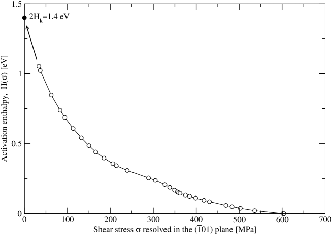
Figure 5.5: Stress dependence of the activation enthalpy calculated by integrating the activation volume as a function of stress (Aono et al.,, 1983) according to Eq. 5.26.

More recently, Hollang et al., (1997) devised a method that allows one to calculate $2H_{k}$ directly from measurements of the dependence of $\ln\dot{\gamma}$ on $1/T_{k}$, an inverse temperature at which the thermal component of the yield stress vanishes. All experimental measurements of the temperature dependence of the yield stress were performed on one sample using the cyclic deformation technique of Ackermann et al., (1983), which removes the ambiguity of interpretation of data obtained from different samples. The rate equation (5.5) implies that the logarithm of the plastic strain rate, $\ln\dot{\gamma}$, is linearly proportional to $1/T_{k}$, since

$$\ln\dot{\gamma}=\ln\dot{\gamma}_{0}-\left(\frac{2H_{k}}{k}\right)\frac{1}{T_{k}}\ ,$$ (5.27)

where $k$ is the Boltzmann constant. Fitting the experimentally measured dependence of $\ln\dot{\gamma}$ on $1/T_{k}$ using Eq. 5.27 yields $2H_{k}=1.27~{}{\rm eV}$, which is in good agreement with the values obtained by extrapolation (Conrad and Hayes,, 1963) and direct integration of the activation volume, Eq. 5.26. Because the experiments of Hollang et al., (1997) represent currently the most accurate studies of the plastic deformation of molybdenum, we will take in the following $2H_{k}=1.27~{}{\rm eV}$ for molybdenum. This value can now be used together with the experimentally measured temperature $T_{k}$ at which the thermal component of the yield stress vanishes (Ackermann et al.,, 1983) to obtain an estimate for $\dot{\gamma}_{0}$. As $T\rightarrow T_{k}$, the activation enthalpy reaches its maximum, $2H_{k}$, and the Arrhenius law suggests that

$$q\equiv\ln(\dot{\gamma}_{0}/\dot{\gamma})=\frac{2H_{k}}{kT_{k}}\ .$$ (5.28)

For a given plastic strain rate $\dot{\gamma}$ and measured temperature $T_{k}$, Eq. 5.28 provides an estimate for $\dot{\gamma}_{0}$. As we mentioned earlier, the mobile dislocation density, included in $\dot{\gamma}_{0}$, is typically a function of temperature and thus $\dot{\gamma}_{0}$ estimated this way is likely to vary as the temperature is lowered. For theoretical calculations, one usually requires an effective value of $\dot{\gamma}_{0}$ that is independent of temperature. This value may be slightly different from that calculated above and can be obtained from the requirement that the theoretically calculated temperature dependence of the yield stress matches the experimental data at high temperatures. In the case of the experiments of Hollang et al., (1997) on molybdenum, this yields $\dot{\gamma}_{0}=3\times 10^{10}~{}{\rm s}^{-1}$ and then $q=31.2$.

For an assumed shape of the Peierls potential, the magnitude of the coefficient $p$ in the line energy of a straight screw dislocation, $V_{0}=p\mu b^{2}$, can be calculated numerically from Eq. 5.13 by requiring that $2H_{k}=1.27\ {\rm eV}$. The magnitude of $p$ depends on the shape of the Peierls potential and will be given explicitly below.

5.3 The Nudged Elastic Band method

Eqs. 5.13 and 5.20, derived in the last chapter, determine the energy of an isolated kink and the activation enthalpy of the critical bow-out representing the saddle-point configuration at high stresses, respectively. We have mentioned that integrations in these equations are performed along the minimum energy path (MEP) that defines the “reaction coordinate” along which the transformation of the dislocation core takes place. In most cases, the direct calculation of these pathways using, for example, molecular dynamics is not realistic, because these transitions occur typically at time scales many orders of magnitude longer than vibrations of atoms. On the other hand, a number of approximate methods have been developed that predict these transition paths from only a few fundamental parameters of the system, such as the shape of the energy surface and the positions of the two low-energy configurations between which the transition takes place. These methods have been very successful in providing the transition paths in a wide variety of problems, such as chemical reactions, conformational changes of molecules, and diffusion in solids (see McKee and Page, (1993) for review). The maximum of the potential energy along the MEP is the saddle-point for motion of the straight dislocation, defining the activation barrier that plays a key role in the harmonic transition state theory (Vineyard,, 1957).

The method that has recently received a considerable attention (Maragakis et al.,, 2002) and that we employ to determine the activation paths and calculate the activation enthalpies for motion of dislocations is the Nudged Elastic Band (NEB) method, put forward by Jónsson et al., (1998) and Henkelman et al., 2000a . Within this method, one works with replicas of the system that are connected together with springs to obtain a discrete representation of the reaction coordinate. In the terminology of the NEB method, the individual replicas of the system are called “images”. The string of $N+2$ images is represented by a chain of states $[\boldsymbol{\xi}_{0},\boldsymbol{\xi}_{1},\boldsymbol{\xi}_{2},\ldots,\boldsymbol{\xi}_{N+1}]$. Two of these images, namely $\boldsymbol{\xi}_{0}$ and $\boldsymbol{\xi}_{N+1}$, are fixed in the two low-energy configurations that represent the initial and target state of the system and the positions of the remaining $N$ images, forming the so-called elastic band, are adjusted by the optimization algorithm. In our case, $\boldsymbol{\xi}_{0}$ is the position of the dislocation in the original and $\boldsymbol{\xi}_{N+1}$ in the target site, and the energy surface is the Peierls potential $V(\boldsymbol{\xi})$ that will be constructed in Section 5.4. The most straightforward way of obtaining the coordinates of the $N$ intermediate images is by connecting the nearest neighbors by identical linear springs and subsequently minimizing the total potential energy, represented by the objective function

$${\cal S}(\boldsymbol{\xi}_{1},\ldots,\boldsymbol{\xi}_{N})=\sum_{i=1}^{N}V(\boldsymbol{\xi}_{i})+\sum_{i=1}^{N+1}\frac{1}{2}k(\boldsymbol{\xi}_{i}-\boldsymbol{\xi}_{i-1})^{2}$$ (5.29)

with respect to the positions of images $\boldsymbol{\xi}_{1},\ldots,\boldsymbol{\xi}_{N}$. This formulation comprises an elastic band of $N$ images connected by nearest-neighbor springs with stiffness $k$.

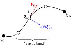
Figure 5.6: Elastic band strung between two fixed images $\boldsymbol{\xi}_{0}$ and $\boldsymbol{\xi}_{N+1}$.

As pointed out by Henkelman et al., 2000a , the method as formulated is not always well-behaved in that the elastic band tends to straighten in the regions where the MEP is curved, and the images tend to slide down toward the fixed endpoints $\boldsymbol{\xi}_{0}$ and $\boldsymbol{\xi}_{N+1}$, which gives a poor resolution of the path close to the saddle-point. It was soon realized that the straightening, or corner-cutting, is caused by the component of the spring force perpendicular to the elastic band, while the down-sliding is caused by the parallel component of the so-called “true force” arising from the potential $V(\boldsymbol{\xi})$. The original idea to avoid these problems is referred to as “nudging” in which each image is subjected only to the component of the spring force parallel to the elastic band and the perpendicular component of the true force. If we denote the unit vector tangent to the elastic band at image $i$ as $\boldsymbol{\hat{\tau}}_{i}$, the force on each image is

$$\boldsymbol{F}_{i}=\boldsymbol{F}_{i\,||}^{s}-\nabla V(\boldsymbol{\xi}_{i})_{\perp}\ ,$$ (5.30)

where $\boldsymbol{F}_{i\,||}^{s}=(\boldsymbol{F}_{i}^{s}\boldsymbol{\hat{\tau}}_{i})\boldsymbol{\hat{\tau}}_{i}$ denotes the parallel component of the spring force at image $i$, and $-\nabla V(\boldsymbol{\xi}_{i})_{\perp}$ is the positive perpendicular component of the true force; see Fig. 5.6. During the minimization, the parallel component of the spring force does not interfere with the perpendicular component of the true force and $\nabla V(\boldsymbol{\xi}_{i})_{\perp}\stackrel{{\scriptstyle{\rm all}~{}i}}{{\longrightarrow}}0$ as the shape of the elastic band approaches the MEP. In the relaxed configuration, the force on each image coincides with the parallel component of the spring force which determines the spacing between individual images along the path. In the simplest version of the NEB method, the parallel component of the spring force is determined by subtracting the forces calculated using the neighboring images:

$$\boldsymbol{F}_{i\,||}^{s}=k\left\{\left[(\boldsymbol{\xi}_{i+1}-\boldsymbol{\xi}_{i})-(\boldsymbol{\xi}_{i}-\boldsymbol{\xi}_{i-1})\right]\boldsymbol{\hat{\tau}}_{i}\right\}\boldsymbol{\hat{\tau}}_{i}\ .$$ (5.31)

The perpendicular component of the true force can be easily obtained by subtracting the component of the true force projected along the elastic band from the total true force vector, i.e.

$$\nabla V(\boldsymbol{\xi}_{i})_{\perp}=\nabla V(\boldsymbol{\xi}_{i})-[\nabla V(\boldsymbol{\xi}_{i})\boldsymbol{\hat{\tau}}_{i}]\boldsymbol{\hat{\tau}}_{i}\ .$$ (5.32)

A convenient way to calculate the unit vector tangent to the elastic band at image $i$ is to bisect the tangents calculated with the help of the two neighboring images,

$$\boldsymbol{\tau}_{i}=\frac{\boldsymbol{\xi}_{i}-\boldsymbol{\xi}_{i-1}}{|\boldsymbol{\xi}_{i}-\boldsymbol{\xi}_{i-1}|}+\frac{\boldsymbol{\xi}_{i+1}-\boldsymbol{\xi}_{i}}{|\boldsymbol{\xi}_{i+1}-\boldsymbol{\xi}_{i}|}\ ,$$ (5.33)

and then normalize, $\boldsymbol{\hat{\tau}}_{i}=\boldsymbol{\tau}_{i}/|\boldsymbol{\tau}_{i}|$. If the spring constant is identical for each image, defining the tangent this way ensures that the images are equispaced, even in regions of a large curvature. In certain cases, mainly when the energy of the system changes rapidly along the path, this method may cause the elastic band to get “kinky” which often results in a slow convergence of the optimization algorithm. To remedy this problem, Henkelman and Jónsson, (2000) devised a new way of defining the local tangent at image $i$. Instead of considering the two neighboring images, $i-1$ and $i+1$, only the image with the higher energy and $i$ are retained in the estimate. Within this improved scheme, the tangent is calculated as

$$\boldsymbol{\tau}_{i}=\left\{\begin{array}[]{ll}\boldsymbol{\tau}_{i}^{+}&{\rm if}\quad V(\boldsymbol{\xi}_{i+1})>V(\boldsymbol{\xi}_{i})\geq V(\boldsymbol{\xi}_{i-1})\\ \boldsymbol{\tau}_{i}^{-}&{\rm if}\quad V(\boldsymbol{\xi}_{i+1})\leq V(\boldsymbol{\xi}_{i})<V(\boldsymbol{\xi}_{i-1})\end{array}\right.\ .$$ (5.34)

If the two neighboring images have both higher or lower energy than that of image $i$, i.e. if $V(\boldsymbol{\xi}_{i+1})>V(\boldsymbol{\xi}_{i})<V(\boldsymbol{\xi}_{i-1})$ or $V(\boldsymbol{\xi}_{i+1})<V(\boldsymbol{\xi}_{i})>V(\boldsymbol{\xi}_{i-1})$, the tangent is determined by a weighted average of the tangents calculated from the two neighboring images:

$$\boldsymbol{\tau}_{i}=\left\{\begin{array}[]{ll}\boldsymbol{\tau}_{i}^{+}\Delta V^{\max}(\boldsymbol{\xi}_{i})+\boldsymbol{\tau}_{i}^{-}\Delta V^{\min}(\boldsymbol{\xi}_{i})&{\rm if}\quad V(\boldsymbol{\xi}_{i+1})>V(\boldsymbol{\xi}_{i-1})\\ \boldsymbol{\tau}_{i}^{+}\Delta V^{\min}(\boldsymbol{\xi}_{i})+\boldsymbol{\tau}_{i}^{-}\Delta V^{\max}(\boldsymbol{\xi}_{i})&{\rm if}\quad V(\boldsymbol{\xi}_{i+1})<V(\boldsymbol{\xi}_{i-1})\end{array}\right.\ ,$$ (5.35)

where

$$\Delta V^{\min}(\boldsymbol{\xi}_{i}) = \min(|V(\boldsymbol{\xi}_{i+1})-V(\boldsymbol{\xi}_{i})|,|V(\boldsymbol{\xi}_{i-1})-V(\boldsymbol{\xi}_{i})|)$$ (5.36)

$$\Delta V^{\max}(\boldsymbol{\xi}_{i}) = \max(|V(\boldsymbol{\xi}_{i+1})-V(\boldsymbol{\xi}_{i})|,|V(\boldsymbol{\xi}_{i-1})-V(\boldsymbol{\xi}_{i})|)$$ (5.37)

and the tangent vectors obtained from (5.34) and (5.35) have to be normalized. This formulation guarantees that the unit tangent $\boldsymbol{\hat{\tau}}_{i}$ varies smoothly as the energies of the two neighboring images get either higher or lower relative to the energy of image $i$, and, therefore, the convergence of the optimization process is not affected by any abrupt changes.

When the restoring forces on the images perpendicular to the path are weak compared to the rapidly changing parallel forces, the images caught in the regions of large parallel forces tend to slide down. However, equal spacing between the images is guaranteed if the springs are identical, and, therefore, the only way the objective function ${\cal S}(\boldsymbol{\xi}_{1},\ldots,\boldsymbol{\xi}_{N})$ can be lowered is by buckling the chain of images into another, nearly force-free region. To avoid this, Jónsson et al., (1998) suggested the use of a smooth switching function that gradually turns on the perpendicular component of the spring force whenever the path becomes kinky. The force on image $i$ is then calculated as

$$\boldsymbol{F}_{i}=\boldsymbol{F}_{i\,||}^{s}-\nabla V(\boldsymbol{\xi}_{i})_{\perp}+f(\phi_{i})\boldsymbol{F}^{s}_{{}_{i}\,\perp}\ ,$$ (5.38)

where $f(\phi_{i})=1/2[1+\cos(\pi\cos\phi_{i})]$ is a switching function that varies between 0 for a straight path and 1 if the adjacent segments joined at image $i$ are at a right angle. In this expression, the angle $\phi_{i}$ is defined as

$$\cos\phi_{i}=\frac{(\boldsymbol{\xi}_{i+1}-\boldsymbol{\xi}_{i})(\boldsymbol{\xi}_{i}-\boldsymbol{\xi}_{i-1})}{|\boldsymbol{\xi}_{i+1}-\boldsymbol{\xi}_{i}|\cdot|\boldsymbol{\xi}_{i}-\boldsymbol{\xi}_{i-1}|}\ .$$ (5.39)

Note, that if there are no kinks along the path, $f(\phi_{i})=0$ for each image $i$, and Eq. 5.38 then becomes identical to Eq. 5.30.

The most recent advancement of the NEB method (Henkelman et al., 2000b, ), called the Climbing Image NEB method (CI-NEB), constitutes a modification of the scheme by introducing variable spring constants and an alternative way of calculating the force on an image, $\boldsymbol{F}_{i}$, which gives a better resolution of the saddle-point configuration. After a few iterations with the conventional NEB method, the image $i_{\max}$ with the highest energy is identified. In further calculations, the force on this image is not given by Eq. 5.30, but rather by

$$\boldsymbol{F}_{i_{\max}}=\nabla V(\boldsymbol{\xi}_{i_{\max}})_{||}\ ,$$ (5.40)

which corresponds to zeroing the spring force on this image completely and including only the inverted parallel component of the true force. The image $i_{\max}$ is thus dragged uphill towards the saddle-point, while the direction of the drag is determined by the position of the two neighboring images.

The NEB method has been used extensively in the present work to calculate the transition paths of the dislocation between two minimum energy configurations. All searches utilize the method of variable spring constants in combination with the switching function defined above. The method is rather insensitive to the chosen range of magnitudes of the spring constants and performed efficiently for all shapes of the Peierls potential. The velocity Verlet algorithm (Allen and Tildesley,, 1987) was used to update the positions of images $\boldsymbol{\xi}_{1}$ to $\boldsymbol{\xi}_{N}$ in each iteration step.

5.4 Construction of the Peierls potential

5.4.1 Peierls stress and Peierls potential

Because $1/2\langle{111}\rangle$ screw dislocations in bcc metals do not have well-defined slip planes and can thus easily cross-slip between different planes of the zone of the slip direction, we will construct the Peierls potential, $V$, as a function of two variables, $x$ and $y$, representing the position of the intersection of the dislocation line with the $\{111\}$ plane perpendicular to the corresponding $\langle{111}\rangle$ slip direction. At 0 K, an isolated screw dislocation moves between two low-energy sites by transforming its core along a minimum energy path, described by a curvilinear coordinate $\xi$ that connects the two potential minima. During this transition, the dislocation surmounts the Peierls barrier $V(\xi)$ that is obtained as a cross-section of the Peierls potential, $V(x,y)$, along $\xi$. Atomistic simulations do not provide the overall form of $V(\xi)$ but merely its maximum slope that is proportional to the Peierls stress, $\sigma_{P}$, at which the dislocation moves. The relation between the Peierls stress and the Peierls barrier is

$$\sigma_{P}b=\max\left(\frac{{\rm d}V(\xi)}{{\rm d}\xi}\right)\ .$$ (5.41)

For a given orientation of the MRSSP, characterized by the angle $\chi$, and the angle the slip plane makes with the most highly stressed $\{110\}$ plane, $\psi$, the Peierls stress can be easily calculated as a projection of the CRSS applied in the MRSSP to the slip plane, i.e. $\sigma_{P}={\rm CRSS}\cos(\chi-\psi)$. Unlike the Peierls stress that is readily obtained from the CRSS found in atomistic studies, there is no direct way of extracting the Peierls barrier, $V(\xi)$, either from experimental data or atomic-level calculations. We will construct the Peierls potential by assuming a certain functional form obeying the symmetry and the periodicity of the lattice, whose height is then parametrized to satisfy Eq. 5.41.

In bcc metals, the Schmid stress is not the only stress component that affects the dislocation glide. As we have seen in Chapter 3, the glide of an isolated screw dislocation in molybdenum displays a significant twinning-antitwinning asymmetry for pure shear and asymmetries related to the effect of the shear stress perpendicular to the slip direction. These features must be reflected in the Peierls potential as well as in the corresponding Peierls barrier $V(\xi)$. One can imagine that non-glide stresses that are responsible for the above-mentioned asymmetries “distort” the Peierls potential in such a way that the glide of the dislocation occurs at either lower or higher stresses than those needed for the glide if the Peierls potential were undistorted.

5.4.2 Symmetry-mapping function

The shape of the Peierls potential will be based on the so-called mapping function that merely captures the three-fold symmetric character of $\{111\}$ planes that are perpendicular to the lines of screw dislocations. This function can be written as a product of three basis functions defined along the three characteristic directions in the $(111)$ plane (for complete derivation, see Appendix C). For the sake of simplicity, we will use a particularly simple sinusoidal forms of the basis functions for which the mapping term reads

$$m(x,y)=\frac{1}{2}+\frac{4}{3\sqrt{3}}\sin{\frac{\pi}{3a_{0}}\left(2y\sqrt{3}+a_{0}\right)}\,\sin{\frac{\pi}{a_{0}}\left(\frac{y}{\sqrt{3}}-x-\frac{a_{0}}{3}\right)}\,\sin{\frac{\pi}{a_{0}}\left(\frac{y}{\sqrt{3}}+x+\frac{2a_{0}}{3}\right)}$$ (5.42)

and is identical to the undeformed Peierls potential of Edagawa et al., (1997). In Eq. 5.42, $(x,y)$ defines the position of the intersection of the dislocation line with the $(111)$ plane, where $x$ coincides with the $[\bar{1}2\bar{1}]$ direction that is a trace of the $(\bar{1}01)$ plane on the $(111)$ plane, and $y=[10\bar{1}]$ is perpendicular to $x$ and to the $[111]$ direction. It can be shown that $m(x,y)$ is a three-fold symmetric function bounded such that $0\leq m\leq 1$. The minima and maxima of $m$ form a triangular lattice with the lattice parameter $a_{0}=a\sqrt{2/3}$ where $a$ is the $\langle{100}\rangle$ lattice parameter.

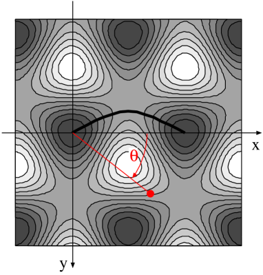
Figure 5.7: Mapping function $m(x,y)$ of the Peierls potential. Dark domains correspond to potential minima and bright domains to potential maxima.

The procedure for constructing the Peierls potential is not unique, and the outlined approach is one possible way. We start by considering first that: (i) the loading is applied as a pure shear acting in the $(\bar{1}01)$ slip plane parallel to the $[111]$ direction, and (ii) the glide commences when this stress reaches the Peierls stress. A consequence of this loading is that the Peierls stress is determined directly by the Schmid law. This provides a good starting point for the construction of the potential that will eventually be modified to take the non-Schmid effects into account. In this first approximation, the Peierls potential is simply

$$V(x,y)=\Delta{V}\,m(x,y)\ ,$$ (5.43)

where $\Delta{V}$ is an unknown height of the potential and $m(x,y)$ is the mapping function (5.42). Considering the case that $\chi=\psi=0$, i.e. loading by pure shear parallel to the $[111]$ direction in the $(\bar{1}01)$ plane, the Peierls stress in Eq. 5.41 is directly equal to the CRSS for $\chi=0$ obtained from atomistic simulations in Chapter 3. Hence, Eq. 5.41 represents a condition that allows one to determine the height of the Peierls potential, $\Delta V$, as follows. For a trial value of $\Delta{V}$, use the NEB method described in Section 5.3 to calculate the MEP between two adjacent potential minima on the $(\bar{1}01)$ plane. Sufficient accuracy has been obtained using a total of fifteen images, where thirteen of them formed the elastic band and the last two were fixed at the beginning and end of the transition path. Since the elastic band determines the contour $\xi$ of the transition path, it is easy to obtain the Peierls barrier, $V(\xi)$, by interpolating the potential values corresponding to the images along the elastic band. One can then differentiate the Peierls barrier and find the maximum. Finally, we evaluate the difference between the left and right side of Eq. 5.41. If the error is large, we adjust $\Delta{V}$ and repeat the whole process. Once the error falls into the specified tolerance, which in our case is $10^{-4}~{}{\rm eV}/{\rm\AA}^{2}$, we terminate the optimization process and $\Delta{V}$ is then the height of the Peierls potential. For molybdenum, this approach yields

$$\Delta{V}=0.0757~{}{\rm eV}/{\rm\AA}\ .$$ (5.44)

5.4.3 Effect of shear stress parallel to the slip direction

If the Peierls potential were stress-independent and had the form defined in the preceding section, the orientation dependence of the CRSS would follow exactly the Schmid law in that ${\rm CRSS}\propto 1/\cos\chi$. As we can see from Fig. 3.6, this is not the case in molybdenum. Provided that only the shear stress parallel to the slip direction is applied, the CRSS varies with the orientation of the MRSSP in such a way that it is higher for the antitwinning shear ($\chi>0$) and lower for the twinning shear ($\chi<0$), relative to the value for $\chi=0$ when the MRSSP coincides with the $(\bar{1}01)$ plane. This orientation dependence of the CRSS implies that the activation barrier for motion of the dislocation is higher for $\chi>0$ and lower for $\chi<0$.

In order to account for the twinning-antitwinning asymmetry, we augment the Peierls potential by an angular-dependent function $V_{\sigma}(\chi,\theta)$ that represents a distortion of the three-fold symmetric basis by a non-glide shear stress parallel to the slip direction. Here, $\theta$ is the angle between the $x$ axis and the line connecting the origin with the point $(x,y)$, as shown in Fig. 5.7. The Peierls potential then reads

$$V(x,y)=\left[\Delta{V}+V_{\sigma}(\chi,\theta)\right]m(x,y)\ .$$ (5.45)

We assume that $V_{\sigma}$ is proportional to the shear stress parallel to the slip direction resolved in the plane defined by the angle $\theta$, i.e. $V_{\sigma}\propto\sigma\cos(\chi-\theta)$. In the case of molybdenum, loading by pure shear parallel to the slip direction always leads to slip on the $(\bar{1}01)$ plane. Hence, the points along the MEP are represented by small angles $\theta$, and this implies that $\cos(\chi-\theta)\propto\cos\theta$. The dependence of $V_{\sigma}$ on the angle $\chi$ will be determined by a dimensionless function $K_{\sigma}(\chi)$. One of the simplest forms of $V_{\sigma}$ is then

$$V_{\sigma}(\chi,\theta)=K_{\sigma}(\chi)\sigma b^{2}\cos\theta\ ,$$ (5.46)

where the factor $b^{2}$ is included to arrive at correct dimension of $V_{\sigma}$. Since $\Delta{V}$ in Eq. 5.45 is already known, we can proceed to determine the $K_{\sigma}(\chi)$ that will recover the twinning-antitwinning asymmetry. For any orientation of the MRSSP, the dislocation subjected to pure shear parallel to the slip direction glides on the $(\bar{1}01)$ plane and thus $\psi=0$. The Peierls stress in Eq. 5.41 can then be written as $\sigma_{P}={\rm CRSS}\cos\chi$, where the CRSS is obtained from the restricted form of the $\tau^{*}$ criterion (4.2) as

$${\rm CRSS}=\frac{\tau_{cr}^{*}}{\cos\chi+a_{1}\cos(\chi+\pi/3)}\ .$$ (5.47)

For each value of $\chi$ and the CRSS obtained from Eq. 5.47, the corresponding $K_{\sigma}$ can be determined as follows. Starting with an initial guess for $K_{\sigma}$ for the given $\chi$, we find the MEP for transition of the dislocation into the adjacent equivalent lattice site on the $(\bar{1}01)$ plane in the potential valley defined by Eq. 5.45. We then extract the Peierls barrier $V(\xi)$ from the set of discrete images along the elastic band, differentiate the Peierls barrier, find its maximum and evaluate the difference between the two sides of Eq. 5.41. If the error is greater than $10^{-4}~{}{\rm eV}/{\rm\AA}^{2}$, we adjust $K_{\sigma}$ and repeat the procedure above. Once the error falls into the specified tolerance, we have found one point of the dependence of $K_{\sigma}$ on $\chi$.

In Fig. 5.8, we show by symbols the data calculated for a set of orientations of the MRSSP. Apparently, $K_{\sigma}(\chi)$ can be described by the linear function

$$K_{\sigma}(\chi)=0.132\chi\ ,$$ (5.48)

in which the coefficient has been obtained by fitting the numerical data, and the angle $\chi$ is in radians. When $\chi=0$, no non-glide stresses are present and the function $K_{\sigma}$ becomes zero. In this case, the dislocation glide is governed by the Schmid law, and the Peierls potential (5.45) reduces to that given by Eq. 5.43. For positive $\chi$, i.e. shearing in the antitwinning sense, $V_{\sigma}$ is positive, and both the Peierls barrier and the Peierls stress for the $(\bar{1}01)$ slip increase relative to $\chi=0$. In contrast, for negative $\chi$, i.e. twinning shear, $V_{\sigma}$ is negative, and both the Peierls barrier and the Peierls stress decrease relative to $\chi=0$. Therefore, Eq. 5.45 represents the Peierls potential that reproduces the twinning-antitwinning asymmetry of glide for loading by the shear stress parallel to the slip direction.

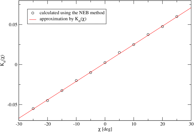
Figure 5.8: Fitting of the $K_{\sigma}(\chi)$ dependence to the values calculated for a discrete set of orientations of the MRSSP.

Upon reversing the sense of shearing, Eq. 5.46 becomes $V_{\sigma}(\chi,\theta)=K_{\sigma}(\chi)(-\sigma)b^{2}\cos\theta$. Since $K_{\sigma}(\chi)$ is odd, $-K_{\sigma}(\chi)\sigma=K_{\sigma}(-\chi)\sigma$, and this implies the well-known result that the reversal of the sense of shearing is identical to keeping the stress positive and reversing the sign of the angle $\chi$. In this case, however, the planes of the $[111]$ zone that were sheared in the twinning sense become sheared in the antitwinning sense and vice versa. Another important point to note is that $V_{\sigma}$ does not obey the translational symmetry of $m(x,y)$, and, when introduced into Eq. 5.45, it causes a breakdown of the translational symmetry of the potential. As a consequence, one has to make sure that the origin of $V(x,y)$ always coincides with the lattice site from which the dislocation moves into the adjacent lattice site. After this elementary step is completed, the origin of $V(x,y)$ must be shifted to this new position, and the search for the minimum energy path can be repeated. This loss of the translational symmetry of the potential is the price that we pay for a particularly simple form of the added term $V_{\sigma}(\chi,\theta)$.

5.4.4 Effect of shear stress perpendicular to the slip direction

To incorporate the effect of the shear stress perpendicular to the slip direction, we will complement $V(x,y)$ in Eq. 5.45 by a term $V_{\tau}(\chi,\theta)$ that represents an angular distortion of the Peierls potential by the shear stress $\tau$ perpendicular to the slip direction. The full form of the Peierls potential involving effects of both non-glide stresses, i.e. shear stress parallel to the slip direction in a plane other than the slip plane and the shear stress perpendicular to the slip direction, then reads

$$V(x,y)=\left[\Delta{V}+V_{\sigma}(\chi,\theta)+V_{\tau}(\chi,\theta)\right]m(x,y)\ .$$ (5.49)

For simplicity, we require that $V_{\tau}$ is a linear function of $\tau$. Furthermore, because the stress tensor (3.2) is invariant with respect to rotations by integral multiples of $\pi$ about the $z$ axis, and since $V_{\tau}$ is a linear function of $\tau$, it follows that $V_{\tau}$ also has to obey the same symmetry. One of the simplest ways to reproduce this symmetry is to write $V_{\tau}$ proportional to $\cos(2\theta+\theta_{0})$, where $\theta_{0}$ is a constant that has to be determined such that $V_{\tau}$ is a linear function of $\tau$. It can be shown that this is true provided $\theta_{0}=\pi/3$, and, therefore, the simplest form that satisfies the above-mentioned requirements is

$$V_{\tau}(\chi,\theta)=K_{\tau}(\chi)\tau b^{2}\cos(2\theta+\pi/3)\ ,$$ (5.50)

where $K_{\tau}(\chi)$ is yet an unknown function. If $\theta_{0}\not=\pi/3$, $K_{\tau}$ would also be an explicit function of $\tau$, and this would make $V_{\tau}$ a nonlinear function of $\tau$. Because $K_{\tau}(\chi)$ is dimensioneless, we have again included in Eq. 5.50 the factor $b^{2}$ that ensures the correct dimension of $V_{\tau}$. In order to keep the calculation of $K_{\tau}$ relatively simple, we considered only two different shear stresses perpendicular to the slip direction, namely $\tau=\pm 0.01C_{44}$. For these stresses, the dislocation glides on the $(\bar{1}01)$ plane, and thus $\psi=0$ for any orientation of the MRSSP. The Peierls stress in Eq. 5.41 can then be written as $\sigma_{P}={\rm CRSS}\cos\chi$, where the CRSS is obtained directly from the full form of the $\tau^{*}$ criterion (4.4) as

$${\rm CRSS}=\frac{\tau_{cr}^{*}-\tau[a_{2}\sin 2\chi+a_{3}\cos(2\chi+\pi/6)]}{\cos\chi+a_{1}\cos(\chi+\pi/3)}\ .$$ (5.51)

The advantage of this approach is that we do not assume a priori that the dislocation can cross-slip into different $\{110\}$ planes as a result of the transformation of its core induced by $\tau$. If the Peierls potential is constructed correctly, this feature would be predicted automatically, which is an important test of the predictive power of the potential.

To determine $K_{\tau}$ corresponding to a given $\chi$, we first fix both $\Delta V$ and $K_{\sigma}$ to the values determined earlier. For a trial value of $K_{\tau}$, we then find the MEP for an elementary $(\bar{1}01)$ jump of the dislocation in the potential valley given by Eq. 5.49. As before, we extract the Peierls barrier $V(\xi)$ along the MEP by interpolating the values calculated from the set of discrete points along the elastic band, differentiate $V(\xi)$, find its maximum slope, and calculate the difference between the two sides of Eq. 5.41 for the CRSS from Eq. 5.51. If the error is large, we adjust $K_{\tau}$ and repeat the process until Eq. 5.41 becomes valid within the desired accuracy.

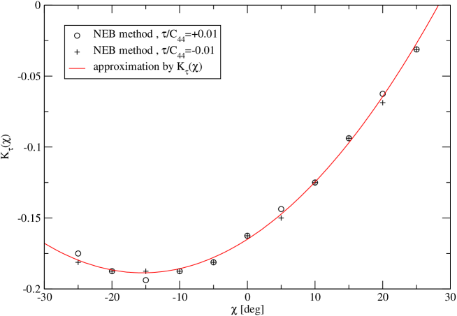
Figure 5.9: Fitting of the $K_{\tau}(\chi)$ dependence from values calculated for a discrete set of orientations of the MRSSPs and two values of $\tau$.

Note, that only two optimization calculations have been performed for each $\chi$, yielding $K_{\tau}(\chi)$ for $\tau=-0.01C_{44}$ and $\tau=+0.01C_{44}$. The variation of $K_{\tau}$ with $\chi$ for these two values of $\tau$ is shown by symbols in Fig. 5.9 and proves that $K_{\tau}$ is independent of $\tau$. As required, $V_{\tau}$ is then a linear function of $\tau$. The curve plotted in this figure represents an approximation of the discrete data and takes on a particularly convenient polynomial form

$$K_{\tau}(\chi)=-0.165+0.173\chi+0.316\chi^{2}\ ,$$ (5.52)

where the angle $\chi$ is in radians. If the angle $\chi$ of the MRSSP is close to $+30^{\circ}$, Fig. 5.9 shows that $K_{\tau}$ virtually vanishes and thus, for this $\chi$, $V(x,y)$ is not distorted by the shear stress perpendicular to the slip direction. Provided that $V(x,y)$ is independent of $\tau$, Eq. 5.41 dictates that the Peierls stress also cannot be a function of $\tau$. This conclusion is consistent with the atomistic data for $\chi=+26^{\circ}$ plotted in Fig. 3.9d showing that the CRSS is almost independent of $\tau$.

Eq. 5.49 represents the final form of the Peierls potential that was constructed to reproduce the 0 K atomistic results from Chapter 3 with the help of the functional form of the effective yield criterion (4.3). In order to keep the fitting procedure reasonably transparent, we considered only two points in each ${\rm CRSS}-\tau$ plot, namely those corresponding to $\tau=\pm 0.01C_{44}$. No fitting has been done for the large $\tau$ regime and, therefore, we do not include a priori any information about the slip of the dislocation on planes other than the $(\bar{1}01)$ plane. Because the ${\rm CRSS}-\tau$ atomistic data vary almost linearly at small $\tau$, the dependence of the Peierls potential on the shear stress perpendicular to the slip direction has also been chosen to be linear. Thus the Peierls potential is likely to reproduce poorly the large $\tau$ regime in which the CRSS values are predicted by linear extrapolation from the regime of small $\tau$. However, as we have shown in Fig. 4.4, this region is virtually inaccessible in real single crystals where another $\{110\}\langle{111}\rangle$ system becomes dominant.

a) $\tau/C_{44}=-0.05$                                            b) $\tau/C_{44}=+0.05$
Figure 5.10: Effect of the shear stress perpendicular to the slip direction, $\tau$, on the shape of $V_{\tau}$. The contours correspond to $V_{\tau}$ given by Eq. 5.50 for $\chi=0$ for which $K_{\tau}$ is negative. Dark regions are negative and bright regions positive values.

The effect of the shear stress perpendicular to the slip direction on the shape of the Peierls potential is shown graphically in Fig. 5.10. The two contour maps show $V_{\tau}$ for positive and negative $\tau$ of the same magnitude, respectively. The dark regions contribute a negative value to the Peierls potential and cause its flattening. On the other hand, bright regions are domains of positive values and result in increase of the height of the potential. It is evident that positive shear stress perpendicular to the slip direction causes lowering of the potential barrier for the slip on the $(\bar{1}01)$ plane and, therefore, makes the slip on this plane easier. This slip mode is suppressed at negative $\tau$, which causes a flattening of the potential along $(\bar{1}10)$ and close to the $(0\bar{1}1)$ plane, while the Peierls barrier along the $(\bar{1}01)$ plane increases. In this case, the slip is more likely to proceed on the $(0\bar{1}1)$ or $(\bar{1}10)$ plane. The slip planes at positive and negative $\tau$ inferred from Fig. 5.10 are identical to those observed in atomistic simulations (see Fig. 3.9) which proves that the predictions made directly from the Peierls potential (5.49) are consistent with the results of 0 K atomistic simulations.

5.5 Correlations of the Peierls potential with results of 0 K atomistic simulations

Because the Peierls potential (5.49) is a function of the orientation of the MRSSP (i.e. angle $\chi$) and both shear stresses parallel and perpendicular to the slip direction, it is instructive to investigate its shape under various loadings. Besides these qualitative tests, the Peierls potential can be used to predict the ${\rm CRSS}-\chi$ and ${\rm CRSS}-\tau$ dependencies that should be in agreement with those determined directly from the $\tau^{*}$ criterion and shown in Fig. 4.4.

In the first test, we will consider the loading by pure shear stress parallel to the $[111]$ direction applied in the MRSSPs determined by angles $\chi=-20^{\circ}$, $\chi=0$, and $\chi=+20^{\circ}$. For this loading, the Peierls potential is given by Eq. 5.45 and the Peierls stress in Eq. 5.41 reads $\sigma_{P}={\rm CRSS}\cos\chi$. Note, that $V(x,y)$ depends explicitly on the actual magnitude of the shear stress parallel to the slip direction, and the shape of the Peierls potential thus evolves with the applied loading.

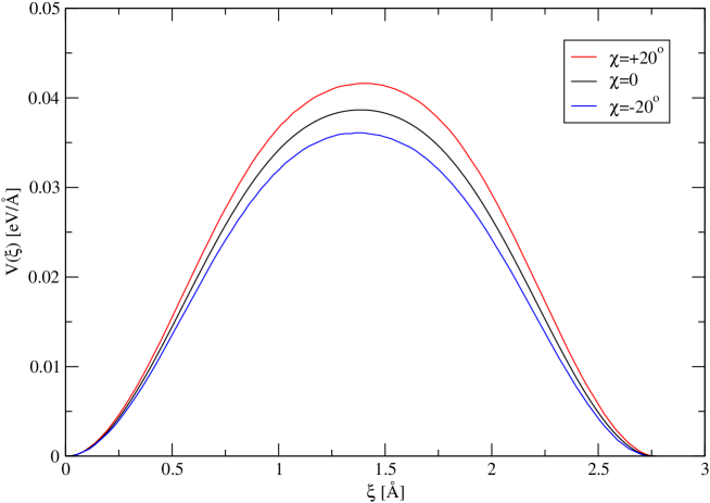
Figure 5.11: The Peierls barrier $V(\xi)$ along the MEP for different angles $\chi$ of the MRSSP of the applied shear stress. The Peierls stress is proportional to the maximum slope of $V(\xi)$.

The Peierls barriers for the three orientations of the MRSSP, calculated from the constructed Peierls potential using the NEB method, are plotted in Fig. 5.11. If the shear stress is applied in the antitwinning sense, i.e. $\chi>0$, the Peierls barrier increases relative to the case when $\chi=0$. The opposite is true for negative $\chi$, i.e. twinning shear, in which case the activation barrier decreases compared to that for $\chi=0$. Because the Peierls stress is proportional to the maximum slope of this barrier, which clearly increases with increasing $\chi$, the potential predicts higher Peierls stress for positive $\chi$ and lower for negative $\chi$. This qualitative trend is consistent with the atomistic simulations in which the CRSS at positive $\chi$ is always higher than that at negative $\chi$. The Peierls potential not only correctly reproduces the twinning-antitwinning asymmetry of shear stress parallel to the slip direction, but also quantitatively agrees with the ${\rm CRSS}-\chi$ dependence calculated from atomistic simulations. This agreement is shown in Fig. 5.12.

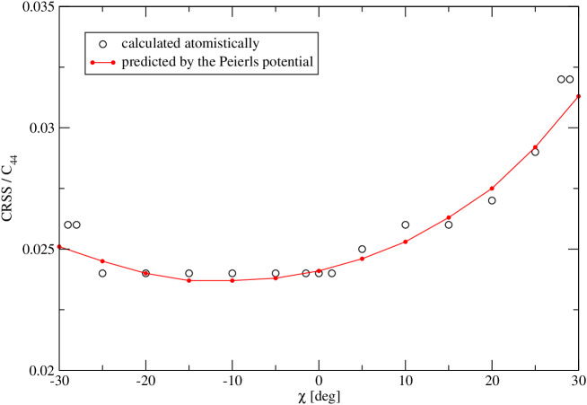
Figure 5.12: Comparison of the orientation dependence of the CRSS calculated atomistically (circles) and predicted from Eq. 5.41 with $\sigma_{P}={\rm CRSS}\cos\chi$.

The second test concerns the effect of a pure shear stress perpendicular to the slip direction on the shape of the Peierls potential and the MEP determined by the NEB method for $(\bar{1}01)$, $(0\bar{1}1)$, and $(\bar{1}10)$ slip. From Fig. 3.8, we know that the shear stress perpendicular to the slip direction changes the structure of the dislocation core such that further glide of the dislocation, induced by the shear stress parallel to the slip direction, occurs at either lower or higher stresses as compared to the case when $\tau=0$. Within the Peierls potential, the transformation of the dislocation core under stress is reproduced via its dependence on both applied shear stresses perpendicular and parallel to the slip direction.

In an unstressed case, the barriers for the motion of the dislocation on the three $\{110\}$ planes are identical, and, therefore, there is no a priori tendency towards glide on any particular plane (see the middle panel in Fig. 5.13). In contrast, positive stress $\tau=+0.05C_{44}$ deforms the Peierls potential such that it develops a low-energy path along the trace of the $(\bar{1}01)$ plane. This modification of the Peierls potential reflects the transformation of the dislocation core by positive $\tau$, which makes the dislocation more glissile in the $(\bar{1}01)$ plane. In contrast, for $\tau=-0.05C_{44}$, the Peierls potential is modified such that the lowest energy path is along the trace of the $(\bar{1}10)$ plane, while the path along the trace of the $(\bar{1}01)$ plane passes through a large Peierls barrier. This is again consistent with the atomistic results, which show that the slip plane for this magnitude of the shear stress perpendicular to the slip direction is the $(\bar{1}10)$ plane. This result is remarkable, since the Peierls potential was constructed by fitting the ${\rm CRSS}-\tau$ data only for $\tau=\pm 0.01C_{44}$, and, therefore, the possibility of glide of the dislocation on any other plane but $(\bar{1}01)$ was not assumed. Hence, the change of the slip plane at negative $\tau$ can be understood as a natural consequence of the asymmetry of the Peierls potential induced by the shear stress perpendicular to the slip direction.

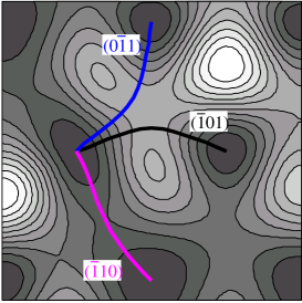
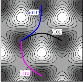
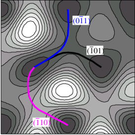
a) $\tau/C_{44}=-0.05$                    b) $\tau/C_{44}=0$                    c) $\tau/C_{44}=+0.05$

Figure 5.13: Shape of the Peierls potential under applied shear stress perpendicular to the slip direction.

Finally, we use the Peierls potential (5.49) to: (i) identify the most operative slip systems in real single crystals of bcc molybdenum in which 12 independent slip systems are present, and (ii) find the critical loadings that mark the onset of slip on each individual system. As in Fig. 4.2, we will consider a set of uniaxial loadings that can be represented in the ${\rm CRSS}-\tau$ plot for MRSSP $(\bar{1}01)$ as a set of straight lines emanating from the origin, with slopes $\eta=\tau/\sigma$. Small values of $\eta$ correspond to uniaxial loadings in the stereographic triangle of the $(\bar{1}01)[111]$ system for which the MRSSP is $(\bar{1}01)$. For larger $|\eta|$, the loading axis rotates into the stereographic triangle of another $\{110\}\langle{111}\rangle$ system, and, therefore, a system other than $(\bar{1}01)[111]$ becomes dominant. For a fixed slope $\eta$ of the loading path in the MRSSP of the $(\bar{1}01)[111]$ system, we can always find the orientations of the MRSSPs corresponding to other $\langle{111}\rangle$ slip directions. As was discussed in Section 4.3, only four such MRSSPs need to be considered in which the resolved shear stress parallel to the slip direction is positive and $-30^{\circ}<\chi<+30^{\circ}$. Since all reference systems are equivalent, the Peierls potential (5.49) applies to any of them. At zero applied stress, the Peierls potential is the same for all four systems, as dictated by symmetry. However, it differs from system to system when the crystal is loaded, since each system is stressed differently. The Peierls potential in each system $\alpha$ is determined by the orientation of the MRSSP, $\chi_{\alpha}$, and the resolved shear stresses perpendicular and parallel to the slip direction, $\tau_{\alpha}$ and $\sigma_{\alpha}$. The ${\rm CRSS}_{\alpha}$ at which a particular $1/2\langle{111}\rangle$ dislocation moves can be predicted from the corresponding Peierls potential by seeking the solution of

$${\rm CRSS}_{\alpha}\,b\cos(\chi_{\alpha}-\psi_{\alpha})=\max\left(\frac{{\rm d}V(\xi)}{{\rm d}\xi}\right)_{\alpha}\ ,$$ (5.53)

where $\psi_{\alpha}$ is the orientation of the slip plane for system $\alpha$. For example, if $(\bar{1}01)[111]$ is the reference system with the highest Schmid stress, $\psi_{\alpha}=0$ for $(\bar{1}01)$, $\psi_{\alpha}=-60^{\circ}$ for $(0\bar{1}1)$, and $\psi_{\alpha}=+60^{\circ}$ for $(\bar{1}10)$ plane. For other reference systems, the orientations of the three possible $\{110\}$ slip planes can be easily deduced from Fig. 4.1.

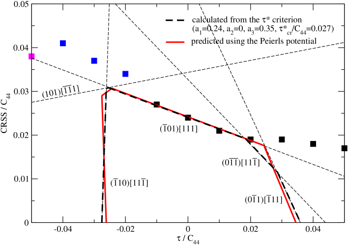
Figure 5.14: Projection of the yield surface calculated from the $\tau^{*}$ criterion (dashed lines) and predicted using the Peierls potential (solid lines) for MRSSP $(\bar{1}01)$.

The four stresses ${\rm CRSS}_{\alpha}$ calculated from Eq. 5.53 and the corresponding shear stresses perpendicular to the slip direction $\tau_{\alpha}=\eta_{\alpha}{\rm CRSS}_{\alpha}$, in the MRSSP given by the angle $\chi_{\alpha}$, can now be mapped back onto the loading path in the MRSSP of the $(\bar{1}01)[111]$ system. This gives four critical points that mark the onset of slip on the four slip systems $\alpha$. If the same calculation is performed for all possible orientations of the loading path, i.e. for $-\infty<\eta<\infty$, the points corresponding to activation of individual slip systems trace the critical lines for these systems. The inner envelope of these lines represents a projection of the yield surface that is plotted in Fig. 5.14 as the solid polygon. Superimposed in Fig. 5.14 are also the critical lines calculated earlier from the $\tau^{*}$ criterion (4.6) and their inner envelope, plotted as the dashed polygon. One can see that the yield surface obtained from the Peierls potential by means of Eq. 5.53 is in full agreement with that calculated from the $\tau^{*}$ criterion. This proves that the predictions made on the basis of the constructed Peierls potential (5.49) are fully consistent with the $\tau^{*}$ criterion, which is itself a close approximation of the results of 0 K atomistic simulations.

5.6 Macroscopic yield behavior predicted by the constructed Peierls potential

The Peierls potential (5.49) will now be used in conjunction with the Dorn-Rajnak expression for the activation enthalpy (5.20), or the model of elastic interaction of kinks (5.23), to predict for single crystals of molybdenum the dependence of the activation enthalpy and the activation volume on the applied stress, and the temperature and strain rate dependence of the yield stress. These calculated dependencies can be readily compared with experimental measurements.

The following calculations will be made for tensile loading along the $[\bar{1}49]$ axis that allows subsequent comparison with tensile experiments by Hollang et al., (1997). For this loading axis, the MRSSP is $(\bar{1}01)$ and $\chi=0$, and the ratio of the two resolved shear stresses is $\eta=\tau/\sigma=0.51$. In the calculation, the loading is expressed as a combination of the shear stresses parallel and perpendicular to the slip direction, where the ratio $\eta$ determines the orientation of the loading path plotted in Fig. 5.15. It is important to emphasize that the loading path first reaches the critical line for the $(\bar{1}01)[111]$ system, which thus becomes the most prominent, and the dislocations will proceed by normal slip on the $(\bar{1}01)$ plane. Moreover, since no other system is activated for slip at the comparatively low CRSS, the macroscopic plastic deformation will correspond to single slip on the $(\bar{1}01)[111]$ system. In other words, the activation enthalpy for the $(\bar{1}01)[111]$ system is markedly lower than those for other slip systems, which will greatly simplify the calculation of the temperature dependence of the yield stress.

For each stress state along the loading path, we can determine the orientation of the MRSSP in the zone of every $\langle{111}\rangle$ direction and thus identify the four $\{110\}\langle{111}\rangle$ reference systems for which the MRSSP lies within the angular region $\chi=\pm 30^{\circ}$ and the shear stress parallel to the slip direction acting in this MRSSP is positive. For each of these systems, the shear stresses perpendicular and parallel to the slip direction are substituted in Eq. 5.49 to determine the Peierls potential in the $\{111\}$ plane of this system. In each case, we find the MEP that connects the original Peierls valley with that of the neighboring minimum energy lattice site and calculate the profile along this MEP, $V(\xi)$. Note, that the dislocation can move into three adjacent lattice sites on planes at $\psi=0$, $\psi=-60^{\circ}$, and $\psi=+60^{\circ}$, marked in Fig. 5.13. For each such contour, one can obtain the activation enthalpy either from the model of the dislocation bow-out (5.20) or from the model of elastic interaction of fully developed kinks (5.23).

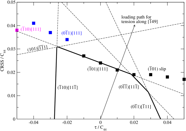
Figure 5.15: Orientation of the loading path corresponding to the tensile loading along $[\bar{1}49]$ used in the experiments of Hollang et al., (1997). The ${\rm CRSS}-\tau$ atomistic data (symbols) and the lines calculated from the $\tau^{*}$ criterion correspond to the MRSSP $(\bar{1}01)$.

At this point, it is important to emphasize that the yield stresses predicted by the model are uniformly about a factor of 3 higher than experiments. This is a well-known discrepancy that appears in all 0 K atomistic simulations of an isolated screw dislocation and that is routinely removed by scaling the theoretical data to reproduce the experimental yield stress extrapolated to 0 K. The physical origin of this discrepancy is explained in detail in Appendix A. This scaling can be easily accomplished by renormalizing the shear stresses in Eqs. 5.20, 5.23, and 5.49, as $\tau=m\tilde{\tau}$ and $\sigma=m\tilde{\sigma}$, where $\tilde{\tau}$ and $\tilde{\sigma}$ are the renormalized shear stresses perpendicular and parallel to the slip direction, respectively. The constant $m=2.9$ was determined by requiring that the yield stress corresponding to zero activation enthalpy (and thus also zero temperature) equals to the experimental yield stress extrapolated to 0 K, i.e. $870\ {\rm MPa}$. For comparisons with experiments given in the following text, we will always use the renormalized stress $\tilde{\sigma}$ given in ${\rm MPa}$ and drop the tilde for brevity.

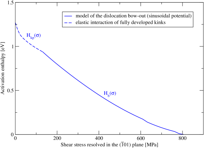
Figure 5.16: Stress dependence of the activation enthalpy for the $(\bar{1}01)[111]$ primary slip system under loading in tension along $[\bar{1}49]$.

The stress dependence of the activation enthalpy for the most prominent slip system, $(\bar{1}01)[111]$, is shown in Fig. 5.16, where the horizontal axis represents the renormalized shear stress $\tilde{\sigma}$ parallel to the $[111]$ slip direction resolved in the $(\bar{1}01)$ plane. At low stresses, the dislocation moves by nucleating a pair of interacting kinks, and the activation enthalpy is given by $H_{kp}$ obtained from Eq. 5.23. In the high-stress regime, the dislocation moves by bowing-out in the direction of the applied stress, and the activation enthalpy, $H_{b}$, is given by Eq. 5.20. In the limit of zero stress, the activation enthalpy approaches the energy of two isolated kinks, $2H_{k}=1.27\ {\rm eV}$.

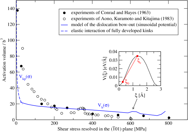
Figure 5.17: Stress dependence of the activation volume for loading in tension along $[\bar{1}49]$. Two different sources of experimental data are plotted for comparison.

The stress dependence of the activation volume calculated by differentiating Eq. 5.20 (high stresses) with respect to the thermal component of the yield stress, $\sigma$, and from Eq. 5.24 (low stresses), is shown in Fig. 5.17, where the symbols correspond to the values measured by Conrad and Hayes, (1963). At intermediate stresses, the calculated activation volume agrees reasonably well with the experiment. The origin of the local maximum close to $600\ {\rm MPa}$, corresponding to a change in the slope of the activation enthalpy at this stress, can be traced back to the shape of the activation barrier. From Fig. 5.4, we can see that the activation enthalpy is proportional to the area bounded between the Peierls barrier and the line with slope $\sigma b$ that is a tangent of the Peierls barrier at $\xi_{0}$. At large stresses, i.e. when $\xi_{0}$ is close to $\xi_{c}$, this area, and thus also the activation enthalpy, increases proportionally to the decrease of the applied stress. At lower stresses, when the position of the critical point $\xi_{c}$ reaches the top of the Peierls barrier (see the inset of Fig. 5.17), the bounded area increases temporarily more rapidly with the decrease of the stress, which gives rise to a change of slope of the activation enthalpy at this stress. Hence, this sudden increase is revealed in the stress dependence of the activation volume as an intermediate maximum, shown in Fig. 5.17 at about $600~{}{\rm MPa}$.

Finally, the temperature dependence of the yield stress can be calculated from the stress dependence of the activation enthalpy plotted in Fig. 5.16. Following Section 5.1, the total plastic strain rate is determined from the Arrhenius law

$$\dot{\gamma}=\dot{\gamma}_{0}\sum_{\alpha}\sum_{\psi}\exp\left(-\frac{H_{b}^{(\alpha,\psi)}(\sigma)}{kT}\right)\ ,$$ (5.54)

where $\dot{\gamma}$ is the total plastic strain rate and $k$ the Boltzmann constant. In general, the summation is carried out over all possible slip planes $\psi=\{0,\pm 60^{\circ}\}$ of those $\{110\}\langle{111}\rangle$ slip systems $\alpha$ that can become activated for slip at the given loading. However, in many cases, one slip system has a markedly smaller activation enthalpy than the others, and, since its activation enthalpy appears in the exponential of (5.54), the contribution of all other slip systems can be neglected. Hence, one arrives at a simple expression of the total plastic strain rate dominated by the most prominent slip system,

$$\dot{\gamma}=\dot{\gamma}_{0}\exp\left(-\frac{H_{b}(\sigma)}{kT}\right)\ ,$$ (5.55)

which gives the activation enthalpy as a function of temperature and plastic strain rate:

$$H_{b}(\sigma)=kT\ln\left(\frac{\dot{\gamma}_{0}}{\dot{\gamma}}\right)\ .$$ (5.56)

It is worthwhile noting that the simple expression (5.56) can be used even when two slip systems have almost equal prominence, i.e. two slip systems have equally small activation enthalpy $H_{b}^{(\alpha,\psi)}(\sigma)$. In this case, the double sum in Eq. 5.54 reduces effectively to a factor of 2, and the activation enthalpy then becomes $H_{b}(\sigma)=kT\ln(2\dot{\gamma}_{0}/\dot{\gamma})=kT\ln 2+kT\ln(\dot{\gamma}_{0}/\dot{\gamma})$. Since $\ln(\dot{\gamma}_{0}/\dot{\gamma})$ is typically 20–40, which is much larger than $\ln 2\ (\approx 0.7)$, the activation enthalpy is still closely approximated by the relation (5.56).

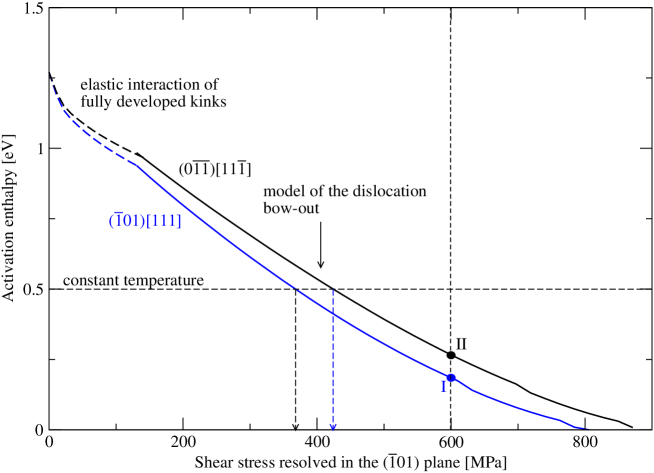
Figure 5.18: Stress dependence of the activation enthalpy for the two most operative slip systems under loading in tension along $[\bar{1}49]$. The labels I and II mark the activation enthalpies calculated for the two systems at $600~{}{\rm MPa}$.

For loading in tension along $[\bar{1}49]$, Fig. 5.18 shows that the calculated activation enthalpy for the $(\bar{1}01)[111]$ system is at any stress $\sigma$ significantly lower than that for the next most operative system, $(0\bar{1}\bar{1})[11\bar{1}]$. This means that, at constant temperature $T$, the $(\bar{1}01)[111]$ system will be activated for slip at a lower applied stress than that needed for operation of the secondary system, $(0\bar{1}\bar{1})[11\bar{1}]$. The order of activation of these two systems is clearly consistent with the $\tau^{*}$ criterion, particularly with Fig. 5.15, where the loading path first reaches the critical line for the $(\bar{1}01)[111]$ primary system, then that for the $(0\bar{1}\bar{1})[11\bar{1}]$ secondary system, etc. Hence, the rate equation (5.54) is clearly dominated by the term involving the activation enthalpy for the $(\bar{1}01)[111]$ system and thus effectively reduces to the single slip rate equation (5.55), where $H_{b}(\sigma)$ is the stress dependence of the activation enthalpy for the $(\bar{1}01)[111]$ primary system.

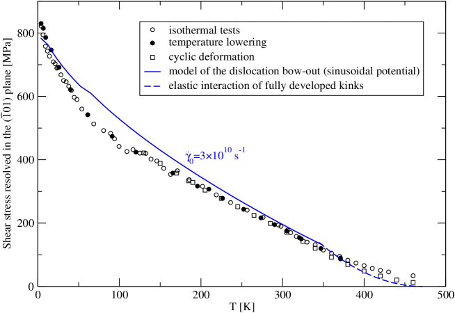
Figure 5.19: Temperature dependence of the yield stress for the $(\bar{1}01)[111]$ system under loading in tension along $[\bar{1}49]$. The solid curve is calculated from the model of the dislocation bow-out using the constructed Peierls potential. The experimental data are from Hollang et al., (2001).

The temperature dependence of the yield stress can now be calculated directly from Eq. 5.56. We will consider the same plastic strain rate as in the experiments of Hollang et al., (1997), $\dot{\gamma}=8.6\times 10^{-4}\ {\rm s}^{-1}$ and, following the estimates in Section 5.2.4, we set $\dot{\gamma}_{0}=3\times 10^{10}~{}{\rm s}^{-1}$. The activation enthalpy can then be written as $H_{b}(\sigma)=qkT$, where $q=\ln(\dot{\gamma}_{0}/\dot{\gamma})=31.2$. For a given temperature $T$, this equation gives $H_{b}(\sigma)$ for which one can find the corresponding yield stress, $\sigma$, from Fig. 5.16. By repeating this calculation for various temperatures, one obtains the temperature dependence of the yield stress that is plotted in Fig. 5.19, where the data measured by Hollang et al., (1997) using three different methods are shown by symbols. The overall trend of $\sigma(T)$ follows the trend of the experimental data. At high temperatures, the predicted yield stress agrees well with the experiment, but, at low temperatures, the theoretical calculations overestimate the experiment. The cause of this deviation can be traced back to the formulation of the mapping function of the Peierls potential, $m(x,y)$, given by Eq. 5.42. While this function has the correct periodicity, its sinusoidal form imposes a specific shape of the Peierls barrier with a sharp maximum (see Fig. 5.11). The effect of the shape of the Peierls barrier on the temperature dependence of the yield stress was studied before by Suzuki et al., (1995), who found that the temperature dependence of the yield stress agrees with experiments if the Peierls potential exhibits a flat maximum.

5.7 Adjustment of the shape of the symmetry-mapping function

When constructing the Peierls potential, we have assumed that the mapping term $m(x,y)$ can be written as a product of three sinusoidal functions. This naturally leads to the Peierls barrier with sharp maximum. In order to arrive at different shapes of the Peierls barriers, consider multiplication of $m$ in Eq. 5.42 by a function $f$ that affects only the immediate neighborhood of each saddle-point of $m$. The final form of the adjusted mapping function will be written as $\hat{f}m$, where we use an operator $\hat{f}$ to emphasize that the function $f$ is applied to every saddle-point of $m$. Since the MEP passes in the neighborhood of a saddle-point of $m$, this operation merely adjusts the maximum of the Peierls barrier. The important feature of this method is that the positions and heights of minima and maxima of $m$ remain unaffected. A simple way to accomplish this perturbation is to define $f$ in terms of the Fermi-Dirac function, as

$$f(r)=1-\frac{\beta}{1+\exp(\frac{r-r_{0}}{\alpha})}\ ,$$ (5.57)

which ranges between $1-\beta/[1+\exp(-r_{0}/\alpha)]$ (for $r=0$) and $1$ (for $r\rightarrow\infty$), and the three adjustable parameters are $\alpha\geq 0$, $\beta\geq 0$ and $r_{0}\in\langle 0,r_{0}^{max}\rangle$, where $r_{0}^{max}$ denotes the maximum acceptable radius for which the adjacent potential extrema are unaffected by $f$. The magnitude of $\beta$ determines the height of $f$; the mapping function is unaffected if $\beta=0$. The parameter $\alpha$ determines the shape of $f$ in that it becomes a sharper function as $\alpha$ gets smaller. Finally, the radius $r_{0}$ defines the position of the inflection point of $f$.

As we mentioned before, $f$ has to be applied at each saddle-point of the mapping function, $m$. These saddle-points are arranged in a triangular lattice with primitive translation vectors $\boldsymbol{t}_{1}=(1,0)a_{0}$ and $\boldsymbol{t}_{2}=(1/2,\sqrt{3}/2)a_{0}$, whose origin is identified with any saddle-point, e.g. $\boldsymbol{t}_{0}=(1/2,-\sqrt{3}/6)a_{0}$. The positions of the saddle-points are then defined by a set of crystallographic vectors $\boldsymbol{t}=\boldsymbol{t}_{0}+k\boldsymbol{t}_{1}+l\boldsymbol{t}_{2}$, where $k,l$ are integers. For the saddle-points located at $\boldsymbol{t}$, the perturbation is a set of radially-symmetric functions $f(|\boldsymbol{r}-\boldsymbol{t}|)$, where the argument simply means the distance from a particular saddle-point determined by integers $k,l$.

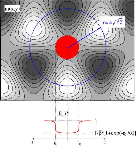
Figure 5.20: Region in which the adjustment of $m$ (contour plot) by the function $f(r)$ takes place. Virtually no change of $m$ takes place beyond $r_{0}$ measured from the saddle-point. The inset below shows the shape of the perturbing function $f(r)$.

In the following, we consider that the parameter $r_{0}$, which controls the radial extent of the saddle-point perturbation, is $r_{0}=a_{0}/(3\sqrt{3})$, which is one-third of the distance from a saddle-point to the nearest maximum/minimum of $m$. This ensures that the perturbation is applied only locally to the given saddle-point and does not affect the adjacent extrema of the potential. The choice of the parameters $\alpha$ and $\beta$ is not unique, but the rule of thumb for their selection is that the mapping function should not lead to sudden potential drops (if $\alpha$ is too small) or intermediate local minima (if $\beta$ is too large). The reasonable values of $\alpha$ are between 0.05 and 0.2, and $\beta$ should be between 0.1 and 0.4. For comparison, Fig. 5.21 shows the contour plots of the product $\hat{f}m$ calculated for: a) $\beta=0$, i.e. without the saddle-point perturbation, and b) $\alpha=0.05$, $\beta=0.2$. The most important feature to notice is that the modified mapping function $\hat{f}m$ (Fig. 5.21b) still possesses the three-fold rotational and the long-range translational symmetry, as required. The proposed perturbation flattens all saddle-points which implies that the activation barrier calculated along the MEP that always passes in the neighborhood of a saddle-point will also exhibit a flat maximum.

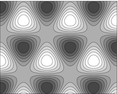
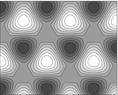
a) $\beta=0$ (no perturbation)                                    b) $\alpha=0.05,\beta=0.2$

Figure 5.21: Contour plots for: (a) unperturbed mapping function $m(x,y)$, and (b) modified mapping function obtained after the perturbation. Different shades in these plots mean different heights of the potential; white regions are potential maxima and black domains potential minima. The values of $\alpha$ and $\beta$ in (b) are chosen such that the change of the mapping function is visible.

5.8 Modified Peierls potential

We stated above that the saddle-point adjustment by the function $f$, Eq. 5.57, modifies only the mapping function $m(x,y)$. The functional forms of all the other terms enclosed in the square bracket of Eq. 5.49, representing the effects of the shear stresses parallel and perpendicular to the slip direction, remain unaffected. In analogy with Eq. 5.49, the modified Peierls potential with adjusted saddle-points of $m$ can now be written as

$$V(x,y)=\left[\Delta{V}+V_{\sigma}(\chi,\theta)+V_{\tau}(\chi,\theta)\right]\hat{f}m(x,y)\ ,$$ (5.58)

where the operator $\hat{f}$ acts on every saddle-point of $m$. It is important to realize that even though the saddle-point perturbation acts only on $m$, the potential height $\Delta V$ and the two adjustable functions $K_{\sigma}(\chi)$ and $K_{\tau}(\chi)$ in Eqs. 5.46 and 5.50 have to be re-fitted.

As already mentioned above, the parameters $\alpha$, $\beta$, $r_{0}$ of the function $f$ (5.57) determine the shape and the extent of the perturbation and must be chosen such that the neighboring potential extrema remain unaffected. In the following, we use $\alpha=0.12$, $\beta=0.2$, $r_{0}=a_{0}/3\sqrt{3}$ for which the saddle-point perturbation leads to the Peierls barrier with a flat maximum. Considering $\chi=0$ and $\tau=0$, and fitting the potential height such that the dislocation moves at the Peierls stress $\sigma_{P}={\rm CRSS}(\chi=0)=0.024C_{44}$, calculated by 0 K atomistic simulations, one arrives at

$$\Delta{V}=0.0787~{}{\rm eV}/{\rm\AA}\ .$$ (5.59)

Similarly, $K_{\sigma}(\chi)$ can be fitted by requiring that the orientation dependence of the shear stress parallel to the slip direction, calculated from Eq. 5.41, reproduces the ${\rm CRSS}-\chi$ dependence in Fig. 3.6. As previously, one again arrives at a linear dependence of $K_{\sigma}$ on $\chi$,

$$K_{\sigma}(\chi)=0.139\chi\ .$$ (5.60)

Finally, the last adjustable function, $K_{\tau}(\chi)$, is determined such that the dependence of the CRSS on the shear stress perpendicular to the slip direction, $\tau$, predicted by Eq. 5.41, reproduces the ${\rm CRSS}-\tau$ data for $\tau=\pm 0.01C_{44}$ and a number of orientations of the MRSSP. As before, $K_{\tau}(\chi)$ can be expressed as a polynomial which now has the form

$$K_{\tau}(\chi)=-0.171+0.182\chi+0.319\chi^{2}\ .$$ (5.61)

We can now perform the same tests for the Peierls potential with flat saddle-points as we have done for the sinusoidal potential earlier in Section 5.5. The Peierls barriers for loading by pure shear parallel to the slip direction acting in three different MRSSPs are shown in Fig. 5.22. In contrast to Fig. 5.11, the maxima of the barriers are now flattened, which results from flat saddle-points of the modified mapping function, $\hat{f}m$. Since the stress to move the dislocation over the barrier is proportional to $\max({\rm d}V/{\rm d}\xi)$, Fig. 5.22 again implies that the CRSS for shearing in the antitwinning sense ($\chi>0$) is higher than the CRSS for shearing in the twinning sense ($\chi<0$), which is consistent with the results of our 0 K atomistic simulations, particularly with Fig. 3.6.

Figure 5.22: The Peierls barrier $V(\xi)$ for slip along the minimum energy path under loading by pure shear stress parallel to the slip direction. The curves are calculated from Eq. 5.41 for the Peierls potential with the saddle-point perturbation, Eq. 5.58.

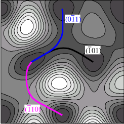
a) $\tau/C_{44}=-0.05$                    b) $\tau/C_{44}=0$                    c) $\tau/C_{44}=+0.05$

Figure 5.23: Shape of the Peierls potential (5.58) with adjusted saddle-points under applied shear stress perpendicular to the slip direction.

The effect of the shear stress perpendicular to the slip direction on the shape of the activation barrier for the motion of the dislocation along the $\{110\}$ planes is qualitatively similar to that discussed for the sinusoidal Peierls potential. For comparison, we show the three minimum energy paths calculated for the Peierls potential (5.58) in Fig. 5.23. The shape of the potential unaffected by $\tau$, shown in Fig. 5.23b, reveals the flattened saddle-points controlled by the parameters $\alpha$, $\beta$, and $r_{0}$. Negative $\tau$ causes the Peierls barrier to flatten along $(\bar{1}10)$ and close to the $(0\bar{1}1)$ plane, see Fig. 5.23a, which lowers the activation barrier for slip on these planes. On the other hand, positive $\tau$ causes flattening of the Peierls barrier along the $(\bar{1}01)$ plane, see Fig. 5.23c, which thus promotes the slip on this plane. These conclusions are again consistent with the results of our 0 K atomistic studies that show a change of the slip plane to $(0\bar{1}1)$ or $(\bar{1}10)$ at negative applied shear stress perpendicular to the slip direction.

5.9 Macroscopic yield behavior predicted by the modified Peierls potential

The macroscopic predictions shown earlier for the sinusoidal potential will now be recalculated using the modified Peierls potential (5.58) with adjusted saddle-points. Since the details of these calculations have been presented already in Section 5.6, we concentrate only on the differences in the results obtained using the two Peierls potentials.

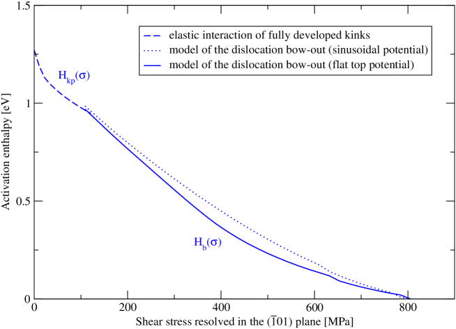
Figure 5.24: Stress dependence of the activation enthalpy for the $(\bar{1}01)[111]$ system under loading in tension along $[\bar{1}49]$.

The stress dependence of the activation enthalpy for tensile loading along $[\bar{1}49]$ is shown in Fig. 5.24, where the solid curve corresponds to the modified Peierls potential and the dotted curve is the dependence obtained previously (Fig. 5.16) for the sinusoidal potential. The curves plotted in this figure again correspond to the primary slip system $(\bar{1}01)[111]$. All other systems have markedly larger activation enthalpies, and their operation can thus be neglected in the following treatment. One can clearly see that the adjustment of the saddle-points affects the gradient of this dependence mainly at intermediate and high stresses. This implies that the temperature dependence of the yield stress will also change significantly which will be apparent mainly at low and intermediate temperatures.

The stress dependence of the activation volume derived from Fig. 5.24 is plotted in Fig. 5.25 by a solid line. This new dependence exhibits a broad plateau close to $300\ {\rm MPa}$ whose origin can be understood with reference to the shape of the activation barrier. As explained earlier, if the position of the activated segment, $\xi_{c}$, at a given stress $\sigma$ meets a point on the activation barrier where its curvature changes rapidly, the activation enthalpy $H_{b}(\sigma)$ suddenly increases with decreasing the applied stress. In our case, the activation barrier has a flat top and so two such points exist, both corresponding to the positions $\xi$ at which $V(\xi)$ drops from its maximum (see the insets of Fig. 5.25). By calculating the position $\xi_{c}$ of the activated segment of the dislocation as a function of $\sigma$, one can see that the plateau and the local maximum in Fig. 5.25 correspond exactly to the two cases where $\xi_{c}$ approaches or leaves the flat top of $V(\xi)$.

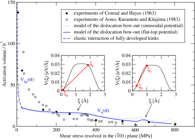
Figure 5.25: Stress dependence of the activation volume for loading in tension along $[\bar{1}49]$. Two different sources of experimental data are plotted for comparison.

Finally, the temperature dependence of the yield stress can be calculated similarly as for the sinusoidal Peierls potential. We have shown earlier that the value of $\dot{\gamma}_{0}$ entering the rate equation (5.56) cannot be calculated by extrapolation from experimental data. Instead, an effective value of this parameter can be conveniently determined by requiring that the temperature dependence of the yield stress, calculated from Eq. 5.41, approaches the experimental data at high temperatures, which gave us $\dot{\gamma}_{0}=3\times 10^{10}~{}{\rm s}^{-1}$. The temperature dependence of the yield stress obtained using the modified Peierls potential (5.58), as well as the previously calculated curve for the sinusoidal potential, are plotted in Fig. 5.26. One can clearly see that the saddle-point perturbation significantly improves the agreement with experiment at low and intermediate temperatures, where the sinusoidal potential led to a substantial disagreement. In other words, if the Peierls potential exhibits flat saddle-points, the top of the activation barrier also flattens, and this then gives rise to a strongly nonlinear temperature dependence of the yield stress that is in good agreement with experiments.

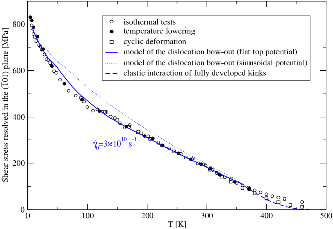
Figure 5.26: Temperature dependence of the yield stress for the $(\bar{1}01)[111]$ system under loading in tension along $[\bar{1}49]$. The experimental data are from Hollang et al., (2001).

5.10 Dislocation glide on higher-index planes

An isolated screw dislocation at 0 K moves by elementary steps on one of the three $\{110\}$ planes in the zone of the $\langle{111}\rangle$ slip direction. This motion is now widely accepted as the mechanism of slip at low temperatures. Nevertheless, it is often argued that the observation of the $\{110\}$ slip in 0 K atomistic simulations does not automatically guarantee that this mechanism of slip holds also at higher temperatures. For example, Seeger and Hollang, (2000) assert that the dislocation core capable of gliding on $\{110\}$ planes at low temperatures undergoes, at approximately 100 K, a transformation to another configuration that can move by elementary steps directly on $\{112\}$ planes. However, this core transformation, as well as the hypothetical elementary steps of the dislocation on $\{112\}$ planes, have never been observed in atomistic simulations, and, therefore, the plane of elementary steps of the dislocation at temperatures above 100 K (for molybdenum) still remains a matter of debate.

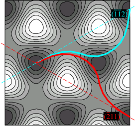
a) minimum energy paths for the two $\{112\}$ jumps

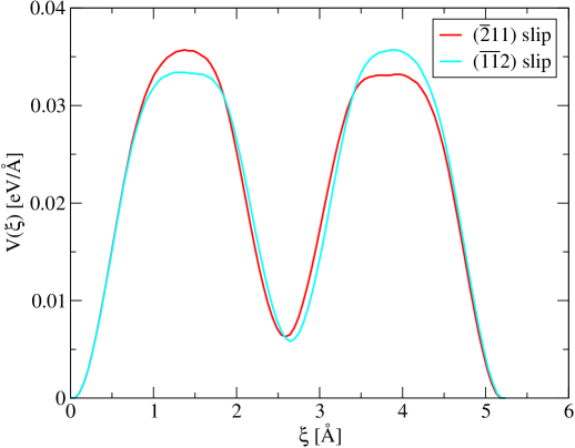
b) Peierls barriers along the MEPs shown in a)

Figure 5.27: Minimum energy paths calculated for two $\{112\}$ jumps using the NEB method (a) and the corresponding Peierls barriers measured along these paths (b).

In order to investigate the glide of the dislocation on $\{112\}$ planes, we calculated the MEPs for slip on the two $\{112\}$ planes in the zone of the $[111]$ slip direction by following the approach introduced earlier for the $\{110\}$ slip. For simplicity, we will discuss here only the case when the MRSSP coincides with the $(\bar{1}01)$ plane and the shear stress perpendicular to the slip direction is zero. Within the NEB method, the minimum energy path for an elementary step of the dislocation on a $\{112\}$ plane can be obtained by providing the original and the target position of the dislocation. In our case, these positions coincide with two adjacent low-energy lattice sites on: (i) the $(\bar{2}11)$ plane at $\psi=+30^{\circ}$, and (ii) the $(\bar{1}\bar{1}2)$ plane at $\psi=-30^{\circ}$. The calculated MEPs for these two transitions are plotted in Fig. 5.27a. Due to the high potential hill on the $(\bar{1}01)$ plane, both MEPs are initially identical and pass around the potential maximum on the $(\bar{1}01)$ plane. After leaving the first (common) saddle-point, the two paths divert and continue to the second saddle-point on the corresponding $\{112\}$ plane, close to the target lattice site.

It is important to realize that the two MEPs are effectively composed of two steps, the first on the $(\bar{1}01)$ plane and the second either on $(0\bar{1}1)$, if the target lattice site lies on the $(\bar{1}\bar{1}2)$ plane, or on $(\bar{1}10)$ if it lies on the $(\bar{2}11)$ plane. Because the Peierls potential is not a function of temperature, one may conclude that the glide of the dislocation proceeds by elementary steps on the two $\{110\}$ planes at any temperature where the plastic flow is induced by thermally activated motion of screw dislocations.

Chapter 6 Temperature and strain rate dependent yield criterion for molybdenum

Problems worthy of attack prove their worth by fighting back.

Paul Erdös

In the previous chapter, we have shown that the Peierls potential developed on the basis of the 0 K effective yield criterion reproduces quite well the experimental measurements of the temperature dependence of the yield stress. For a given orientation of the loading axis, the calculation of the stress dependence of the activation enthalpy requires the following steps: (i) identification of potentially operative slip systems, (ii) calculation of shear stresses parallel and perpendicular to the slip direction for each potentially operative system, (iii) searching the MEP for slip on the three $\{110\}$ planes of each system, and (iv) numerical integration of the activation barriers along these MEPs. For practical calculations of macroscopic flow characteristics, it is highly desirable to carry out these numerical calculations only once and approximate the obtained dependencies using sufficiently accurate analytical relations. This idea is not new and was originally used for formulations of the phenomenological laws of plastic deformation (Kocks et al.,, 1975). Using the approximate expression for the activation enthalpy, one can obtain the temperature dependence of the yield stress by virtue of the formula $H(\sigma)=qkT$, where $q=\ln(\dot{\gamma}_{0}/\dot{\gamma})$ is a constant and $H(\sigma)$ is the obtained analytical expression for the stress dependence of the activation enthalpy. If we now write the yield stress $\sigma$ as a function of $\tau^{*}_{cr}$ and substitute this into the relation $H(\sigma)=qkT$, we arrive at the temperature and strain rate dependent effective yield stress, $\tau^{*}_{cr}(T,\dot{\gamma})$.

6.1 Restricted model for slip at low temperatures

The key step that will allow us later to obtain the closed-form expression for the temperature and strain rate dependence of the yield stress is to approximate the stress dependence of the activation enthalpy using a simple analytical formula. An important requirement imposed on this equation is its invertibility, i.e. the possibility to express the yield stress $\sigma$ as an explicit analytical function of other parameters. For the sake of simplicity, we will initially consider loading by pure shear stress parallel to the $[111]$ slip direction acting in the MRSSP whose orientation is given by the angle $\chi$. We will consider a minimal set of three discrete angles $\chi$, namely $\chi=0$ and $\chi=\pm 20^{\circ}$, that essentially cover the region of orientations $-30^{\circ}<\chi<+30^{\circ}$. Recall, that for any orientation of the applied shear stress, the dislocation always moves on the $(\bar{1}01)$ plane. For a given angle $\chi$, we calculate the stress dependence of the Dorn-Rajnak activation enthalpy, $H_{b}(\sigma)$, for an elementary jump of the dislocation on the $(\bar{1}01)$ plane according to Eq. 5.20. This yields three sets of data points corresponding to $\chi=\{-20^{\circ},0^{\circ},+20^{\circ}\}$ that are plotted in Fig. 6.1 in non-dimensional logarithmic representation. Here, $2H_{k}=1.27~{}{\rm eV}$ is the energy of two isolated kinks. As the applied stress $\sigma$ approaches zero, i.e. $\ln(\sigma/C_{44})\rightarrow-\infty$, $H_{b}(\sigma)\rightarrow 2H_{k}$ and $\ln[1-H_{b}(\sigma)/2H_{k}]\rightarrow-\infty$. At high stresses, as $\sigma$ approaches its maximum, $H_{b}(\sigma)\rightarrow 0$ and $\ln[1-H_{b}(\sigma)/2H_{k}]\rightarrow 0$. The fact that $\ln[1-H_{b}(\sigma)/2H_{k}]$ increases monotonically with $\ln(\sigma/C_{44})$ suggests that a simple analytical expression for the stress dependence of the activation enthalpy can be constructed.

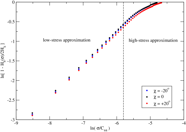
Figure 6.1: Stress dependence of the activation enthalpy calculated from the model of the dislocation bow-out, developed in Section 5.2.2. The yield stress, $\sigma$, is expressed as the CRSS applied in the MRSSP determined by the angle $\chi$.

The goal is now to approximate the dependencies shown in Fig. 6.1 using primitive functions that can be inverted to obtain a simple expression for the yield stress $\sigma$. Due to the change in the slope of the curve, it is necessary to consider two functional forms. At low stresses, the dependence is almost linear which allows us to write

$$\ln\left[1-\frac{H_{b}(\sigma)}{2H_{k}}\right]=\ln{a}+b\ln\left(\frac{\sigma}{C_{44}}\right)\ ,$$ (6.1)

where $a$ and $b$ are two adjustable parameteres. At high stresses, one could in principle use the same functional form with different parameters $a$ and $b$. However, this regime is more closely approximated by an exponential

$$\ln\left[1-\frac{H_{b}(\sigma)}{2H_{k}}\right]=\ln{a^{\prime}}-b^{\prime}{\rm e}^{-\sigma/C_{44}}\ ,$$ (6.2)

where we explicitly use the minus sign in front of the second term in the right-hand side to emphasize the concave character of the function. For each of the three angles $\chi$, the coefficients $a,b$ are determined by fitting the low-stress data plotted in Fig. 6.1. Similarly, the other two coefficients, $a^{\prime}$ and $b^{\prime}$, are determined by fitting the high-stress data. The cross-over between the low and the high stress regime is approximately at $\ln(\sigma/C_{44})\approx-5.8$ which corresponds to $\sigma/C_{44}\approx 0.003$. The coefficients $a,b,a^{\prime},b^{\prime}$ for the two approximations are given numerically in Appendix D.

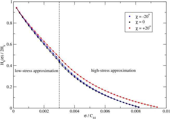
Figure 6.2: Stress dependence of the activation enthalpy calculated from the model of the dislocation bow-out (dots). The curves are calculated from Eq. 6.3.

The difference in the data for the three angles $\chi$, plotted in Fig. 6.1, implies that the stress dependence of the activation enthalpy depends on the orientation of the MRSSP and, therefore, the four coefficients $a,b,a^{\prime},b^{\prime}$, obtained by fitting, are clearly functions of the angle $\chi$. Since we now have for each coefficient three values, corresponding to the three angles $\chi=\{-20^{\circ},0,+20^{\circ}\}$, we can approximate the dependence of each coefficient on $\chi$ by a cubic polynomial. For example, $a(\chi)=a_{0}+a_{1}\chi+a_{2}\chi^{2}$, where the constants $a_{0},a_{1},a_{2}$ are determined by fitting. Finally, the approximate expression for the stress dependence of the activation enthalpy can be obtained from Eqs. 6.1 and 6.2, and reads

$$\frac{H_{b}(\sigma)}{2H_{k}}=\left\{\begin{array}[]{ll}1-a(\chi)\left(\sigma/C_{44}\right)^{b(\chi)}&,\quad{\rm for}\ \sigma/C_{44}\leq 0.003\\ 1-a^{\prime}(\chi)\exp\left[-b^{\prime}(\chi)(\sigma/C_{44})^{-1}\right]&,\quad{\rm for}\ \sigma/C_{44}\geq 0.003\ .\end{array}\right.$$ (6.3)

The stress dependencies of the activation enthalpy, $H_{b}(\sigma)/2H_{k}$, predicted from Eq. 6.3, are shown in Fig. 6.2 as solid lines; the dots correspond to the data plotted in Fig. 6.1. The excellent agreement with the data calculated directly from the model of the dislocation bow-out (Section 5.2.2) proves that Eq. 6.3 is indeed a good approximation of the stress dependence of the activation enthalpy for a wide range of orientations of the MRSSP. As the applied stress approaches zero, the activation enthalpy becomes equal to the energy of two isolated kinks, $2H_{k}$. At large stresses approaching the Peierls stress, the activation enthalpy vanishes and the dislocation is moved purely mechanically by the action of the applied stress.

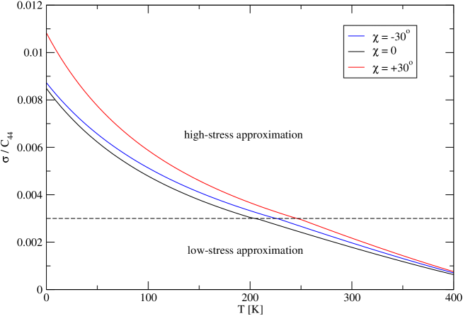
Figure 6.3: Temperature dependence of the shear stress $\sigma$ parallel to the slip direction and acting in the MRSSP, as predicted from Eq. 6.4.

The temperature dependence of the yield stress $\sigma$ can now be obtained by recalling the Arrhenius law for the total plastic strain rate, Eq. 5.5. For a given temperature $T$, the activation enthalpy can be written as $H_{b}(\sigma)=qkT$. Substituting $H_{b}(\sigma)$ from Eq. 6.3 and recovering $\sigma$ then provides the temperature and strain rate dependence of the yield stress:

$$\sigma/C_{44}=\left\{\begin{array}[]{ll}\left[\frac{1-qkT/2H_{k}}{a(\chi)}\right]^{1/b(\chi)}&,\quad{\rm for}\ \sigma/C_{44}\leq 0.003\\ -b^{\prime}(\chi)\left/\ln\left[\frac{1-qkT/2H_{k}}{a^{\prime}(\chi)}\right]\right.&,\quad{\rm for}\ \sigma/C_{44}\geq 0.003\ .\end{array}\right.$$ (6.4)

This dependence is shown graphically in Fig. 6.3 for $\chi=0$ and $\chi=\pm 30^{\circ}$ that represent the boundaries of the angular region of all independent orientations of the MRSSP. The most important feature to note is that non-glide stresses, although so far only those parallel to the slip direction, play an important role at low temperatures and gradually weaken as the temperature is raised. This can be clearly seen on the magnitudes of $\sigma$ for the three MRSSPs which are very different at low temperatures but virtually identical as $T\rightarrow 400~{}{\rm K}$. At $T=0~{}{\rm K}$, larger shear stress is needed to move the dislocation on the $(\bar{1}01)$ plane if the crystal is sheared in the antitwinning sense ($\chi>0$) than if the shear is applied in the twinning sense ($\chi<0$). This observation is fully consistent with the results of our 0 K atomistic simulations, particularly with Fig. 3.6.

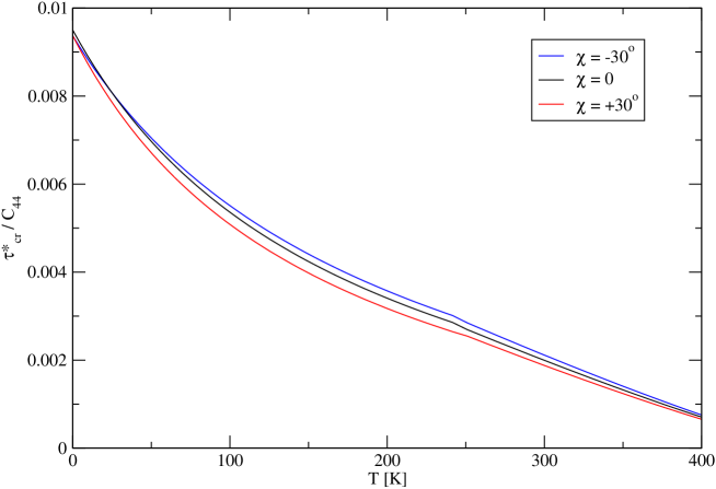
Figure 6.4: Temperature dependence of $\tau^{*}_{cr}$ predicted from Eq. 6.5.

The expression for the temperature and strain rate dependence of the effective yield stress, $\tau^{*}_{cr}(T,\dot{\gamma})$ can now be obtained by noting that, within the restricted model, $\tau^{*}_{cr}$ can be written as a product $\tau^{*}_{cr}=\sigma\,t(\chi)$, where $t(\chi)=\cos\chi+a_{1}\cos(\chi+\pi/3)$ and $\sigma$ is the yield stress. Substituting $\sigma$ from Eq. 6.4 yields

$$\tau^{*}_{cr}/C_{44}=\left\{\begin{array}[]{ll}t(\chi)\left[\frac{1-qkT/2H_{k}}{a(\chi)}\right]^{1/b(\chi)}&,\quad{\rm for}\ \sigma/C_{44}\leq 0.003\\ -b^{\prime}(\chi)t(\chi)\left/\ln\left[\frac{1-qkT/2H_{k}}{a^{\prime}(\chi)}\right]\right.&,\quad{\rm for}\ \sigma/C_{44}\geq 0.003\ .\end{array}\right.$$ (6.5)

The temperature dependence of $\tau^{*}_{cr}$ for the three angles $\chi$ is shown in Fig. 6.4. In contrast to $\sigma(T)$, plotted in Fig. 6.3, $\tau^{*}_{cr}$ is almost independent of the orientation of the MRSSP, and, therefore, Eq. 6.5 can be closely approximated as a function of temperature and strain rate only, without any dependence on $\chi$.

6.2 Full model for slip at low temperatures

The extension of the restricted model presented in the last section to account for the effect of the shear stress perpendicular to the slip direction can now be developed in a straightforward manner. For the sake of simplicity, we will consider three different combinations of the shear stresses perpendicular and parallel to the slip direction applied in the three MRSSPs at $\chi=\{-20^{\circ},0,+20^{\circ}\}$, namely $\eta=\{-0.5,0,+0.5\}$, where $\eta=\tau/\sigma$ and $\tau$ is the shear stress perpendicular to the slip direction. It is important to realize that for any combination of $\chi$ and $\eta$ from these sets, the dislocation always moves on the $(\bar{1}01)$ plane, and, therefore, one does not have to consider the possibility of the glide of the dislocation on the other two $\{110\}$ planes of the $[111]$ zone. The activation enthalpy for an elementary step of the dislocation on the $(\bar{1}01)$ plane can be calculated directly from Eq. 5.20, the only difference from the loading by pure shear parallel to the slip direction being that now the Peierls potential changes shape due to both shear stresses perpendicular and parallel to the slip direction.

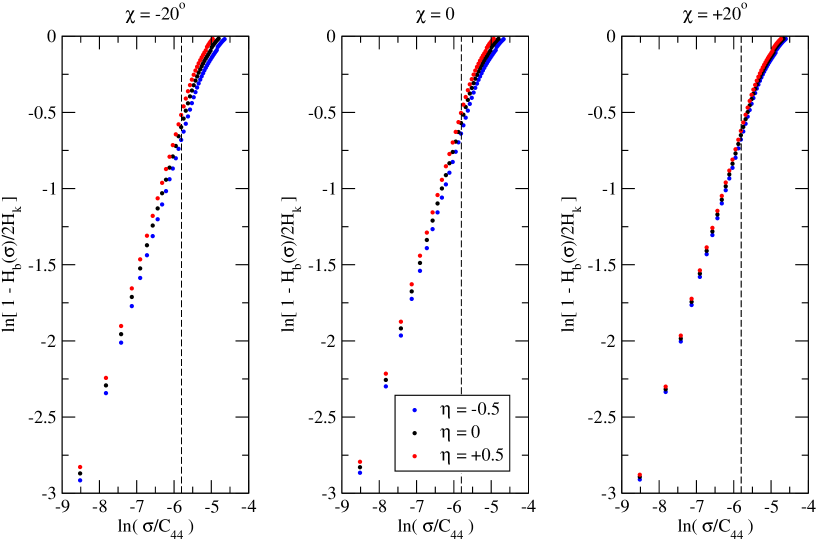
Figure 6.5: Stress dependence of the activation enthalpy calculated using the model of the dislocation bow-out for $\chi=\{-20^{\circ},0,+20^{\circ}\}$ and $\eta=\{-0.5,0,0.5\}$.

The stress dependence of the activation enthalpy calculated from the model of the dislocation bow-out (Section 5.2.2) for all nine combinations of $\chi$ and $\eta$ from the sets above is shown in Fig. 6.5. One can again see that, if the dependence is plotted in logarithmic representation, the low stress behavior can be accurately approximated by a straight line, whereas the high-stress regime has to be described using an inverse exponential. Moreover, the effect of the shear stress perpendicular to the slip direction is significant for $\chi=-20^{\circ}$ but almost vanishes for $\chi=+20^{\circ}$. This observation is consistent with the results of 0 K atomistic simulations plotted in Fig. 3.9a-d, where the slope $|\partial{{\rm CRSS}}/\partial{\tau}|_{\tau=0}$ is largest for negative $\chi$ and almost vanishes at positive $\chi$. Furthermore, the fact that the shear stress perpendicular to the slip direction, i.e. nonzero value of $\eta$, does not lead to the change of the shape of the dependence in Fig. 6.5 implies the same approximate forms for the activation enthalpy as used in the restricted model in Section 6.1. The only additional complication in this case is that the coefficients $a,b$ in the low-stress approximation, and $a^{\prime},b^{\prime}$ in the high-stress approximation, are generally functions of both $\chi$ and $\eta$, i.e.

$$\frac{H_{b}(\sigma)}{2H_{k}}=\left\{\begin{array}[]{ll}1-a(\chi,\eta)\left(\sigma/C_{44}\right)^{b(\chi,\eta)}&,\quad{\rm for}\ \sigma/C_{44}\leq 0.003\\ 1-a^{\prime}(\chi,\eta)\exp\left[-b^{\prime}(\chi,\eta)(\sigma/C_{44})^{-1}\right]&,\quad{\rm for}\ \sigma/C_{44}\geq 0.003\ .\end{array}\right.$$ (6.6)

Each of the four functions $a,b,a^{\prime},b^{\prime}$ can again be expressed as a second-order polynomial in $\chi$ with coefficients defined by another second-order polynomial in $\eta$. For example,

$$a(\chi,\eta)=a_{0}(\eta)+a_{1}(\eta)\chi+a_{2}(\eta)\chi^{2}\ ,$$ (6.7)

where the coefficient functions $a_{0}(\eta)$, $a_{1}(\eta)$ and $a_{2}(\eta)$ can be written as

$$\left[\begin{array}[]{c}a_{0}\\ a_{1}\\ a_{2}\end{array}\right]=\left[\begin{array}[]{ccc}a_{00}&a_{01}&a_{02}\\ a_{10}&a_{11}&a_{12}\\ a_{20}&a_{21}&a_{22}\end{array}\right]\left[\begin{array}[]{c}1\\ \eta\\ \eta^{2}\end{array}\right]\ .$$ (6.8)

The remaining three functions $b,a^{\prime},b^{\prime}$ can be expressed in a similar fashion. Note, that $a_{ij}$ in Eq. 6.8 are independent adjustable constants that have to be determined by fitting the stress dependence of the activation enthalpy shown in Fig. 6.5. Since we have calculated $H_{b}(\sigma)$ for three different angles $\chi$ and three ratios $\eta$, we have exactly nine conditions required for each low and high stress approximation that are needed to determine the constants $a_{ij}$, $b_{ij}$, $a^{\prime}_{ij}$, $b^{\prime}_{ij}$ unambiguously. For convenience, we list the numerical values of these coefficients in Appendix D.

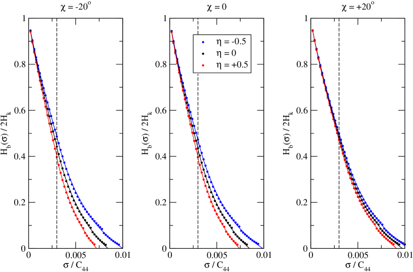
Figure 6.6: Stress dependence of the activation enthalpy calculated using the model of the dislocation bow-out (dots) and from the approximation (6.6) (curves).

The accuracy of fitting the stress dependence of the activation enthalpy by Eq. 6.6 can be easily checked by calculating the dependence $H_{b}(\sigma)$ directly from this equation and comparing it with the data shown in Fig. 6.5. This comparison is presented in Fig. 6.6, where the dots represent the original data calculated from the model of the dislocation bow-out (Section 5.2.2) and the lines are the approximations calculated from Eq. 6.6. The magnitudes of the yield stress $\sigma$, corresponding to zero activation enthalpy, agree well with the values of the CRSS obtained from atomistic studies on a single isolated screw dislocation at 0 K. For example, if the MRSSP lies at $\chi=0$ and $H_{b}(\sigma)=0$, one can clearly see that $\sigma(\eta=-0.5)>\sigma(\eta=0)>\sigma(\eta=+0.5)$, and the yield stress at negative $\tau$ is thus larger than that at positive $\tau$. This conclusion is consistent with the ${\rm CRSS}-\tau$ data plotted in Fig. 3.9a. The same is true for the remaining two angles $\chi$.

The temperature dependence of the yield stress, $\sigma$, can be obtained similarly as in the restricted model presented in the previous section. Substitution of $H_{b}(\sigma)$ from Eq. 6.6 into the relation $H_{b}(\sigma)=qkT$ yields

$$\sigma/C_{44}=\left\{\begin{array}[]{ll}\left[\frac{1-qkT/2H_{k}}{a(\chi,\eta)}\right]^{1/b(\chi,\eta)}&,\quad{\rm for}\ \sigma/C_{44}\leq 0.003\\ -b^{\prime}(\chi,\eta)\left/\ln\left[\frac{1-qkT/2H_{k}}{a^{\prime}(\chi,\eta)}\right]\right.&,\quad{\rm for}\ \sigma/C_{44}\geq 0.003\ .\end{array}\right.$$ (6.9)

For convenience, we plot in Fig. 6.7 the temperature dependence of $\sigma$ calculated for nine different combinations of $\chi$ and $\eta$ from the sets $\chi={-30^{\circ},0,+30^{\circ}}$ and $\eta={-1,0,1}$. At low temperatures, the non-glide stresses play dominant role in that the magnitude of $\sigma$ strongly depends on both $\chi$ and $\eta$. The range of stresses at 0 K is now much wider than that calculated from the restricted model and plotted in Fig. 6.3, which is due to nonzero shear stress perpendicular to the slip direction. As the temperature increases, all stresses gradually decay and thus the importance of the non-glide stresses diminishes.

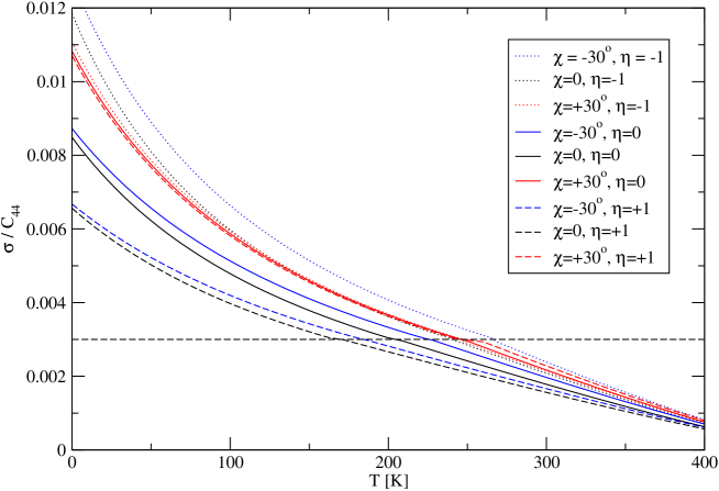
Figure 6.7: Temperature dependence of the yield stress $\sigma$, acting in the MRSSP, as calculated from Eq. 6.9 for three different angles $\chi$ and three ratios $\eta$.

At this point, it is important to emphasize that Fig. 6.7 shows the temperature dependence of the yield stress, $\sigma$, corresponding to a set of limiting combinations of $\chi$ and $\eta$. Due to the crystal symmetry, it is sufficient to consider the MRSSPs in the angular region $-30^{\circ}\leq\chi\leq+30^{\circ}$. Similarly, $-1\leq\eta\leq 1$ defines the bounds of the loading paths plotted in the ${\rm CRSS}-\tau$ projection for which $(\bar{1}01)[111]$ is the most operative $\{110\}\langle{111}\rangle$ system. If $|\eta|>1$, which means that the magnitude of shear stress perpendicular to the slip direction is larger than the corresponding shear stress parallel to the slip direction, Fig. 4.4a-c imply that another $\{110\}\langle{111}\rangle$ system becomes most operative. Importantly, the ratio $\eta$ calculated for the MRSSP of this latter system always falls into the bounds $\langle-1;1\rangle$ unless the loading axis is very close to the $[\bar{1}11]$ corner of the stereographic triangle (see Fig. 4.11). Since all $\{110\}\langle{111}\rangle$ systems are mutually equivalent and provided that we know both the angle $\chi$ and the corresponding ratio $\eta$ for each of these systems, Fig. 6.7 can be used to find the magnitude of the shear stress parallel to the slip direction for which each individual $\{110\}\langle{111}\rangle$ system becomes operative at temperature $T$ and strain rate $\dot{\gamma}$.

Finally, Eq. 6.9 can be used to derive the temperature and strain rate dependent effective yield stress, $\tau^{*}_{cr}(T,\dot{\gamma})$. In this case, $\tau^{*}_{cr}=\sigma t(\chi,\eta)$, where $t(\chi,\eta)=\cos\chi+a_{1}\cos(\chi+\pi/3)+\eta[a_{2}\sin 2\chi+a_{3}\cos(2\chi+\pi/6)]$ is now a function of both the angle of the MRSSP, $\chi$, and the ratio $\eta=\tau/\sigma$. Substituting in this equation the shear stress $\sigma$ from Eq. 6.9 yields

$$\tau^{*}_{cr}/C_{44}=\left\{\begin{array}[]{ll}t(\chi,\eta)\left[\frac{1-qkT/2H_{k}}{a(\chi,\eta)}\right]^{1/b(\chi,\eta)}&,\quad{\rm for}\ \sigma/C_{44}\leq 0.003\\ -b^{\prime}(\chi,\eta)t(\chi,\eta)\left/\ln\left[\frac{1-qkT/2H_{k}}{a^{\prime}(\chi,\eta)}\right]\right.&,\quad{\rm for}\ \sigma/C_{44}\geq 0.003\ .\end{array}\right.$$ (6.10)

This is the sought expression for the effective yield stress $\tau^{*}_{cr}(T,\dot{\gamma})$ that is plotted for $q=31.2$ in Fig. 6.8. In contrast to $\sigma-T$, shown in Fig. 6.7, that was strongly dependent on non-glide stresses within a broad range of temperatures, $\tau^{*}_{cr}$ depends on both $\chi$ and $\eta$ at intermediate temperatures but this dependence almost vanishes close to 0 K and 400 K.

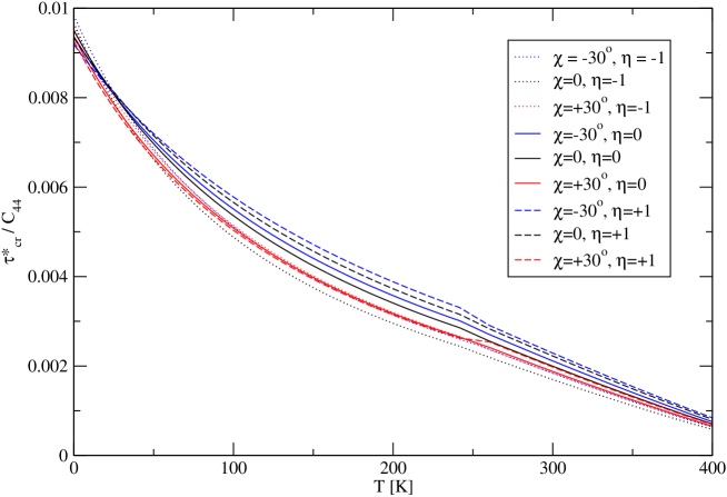
Figure 6.8: Temperature dependence of the effective yield stress, $\tau^{*}_{cr}$, calculated for a fixed strain rate (corresponding to $q=31.2$) and various combinations of $\chi$ and $\eta$.

If the shear stress perpendicular to the slip direction is very different from zero, $\tau^{*}_{cr}$ is not only a function of temperature and strain rate but, at intermediate temperatures, also quite strong function of both $\chi$ and $\eta$. This is best illustrated by realizing that the range of values of $\tau^{*}_{cr}$ close to 200 K is $\Delta\tau^{*}_{cr}=0.001C_{44}$ which, for molybdenum, is approximately 100 MPa. This value represents the maximum error that may occur if one neglects the dependence of $\tau^{*}_{cr}$ on $\eta$.

6.3 High temperature, low stress regime

At high temperatures, the configuration corresponding to the saddle-point energy consists of a pair of fully developed interacting kinks at a finite distance $\Delta{z}$, whose attraction is opposed by the applied Schmid stress. The activation enthalpy to nucleate this critical configuration is given by Eq. 5.23, and, when substituted into $H_{kp}(\sigma)=qkT$, provides the temperature and strain rate dependence of the yield stress $\sigma$, i.e. the shear stress parallel to the slip direction applied in the MRSSP with angle $\chi$:

$$\sigma=\frac{2\pi}{a_{0}^{3}\cos(\chi-\psi)}\frac{(2H_{k})^{2}}{\mu b^{3}}\left(1-\frac{qkT}{2H_{k}}\right)^{2}\ .$$ (6.11)

Here, $\psi$ is the angle of the slip plane, and $a_{0}$ the distance between two adjacent sites in the slip plane. For example, if we consider that the dislocation at elevated temperatures moves by elementary jumps on the $\{110\}$ plane, similarly as at low temperatures, $a_{0}=a\sqrt{2/3}$, where $a$ is the $\langle{100}\rangle$ lattice parameter. The temperature and strain rate dependence of the effective yield stress, $\tau^{*}_{cr}(T,\dot{\gamma})$, can then be obtained the same way as in the low-temperature approximations presented in Sections 6.1 and 6.2. Noting that $\tau^{*}_{cr}=\sigma\,t(\chi,\eta)$, where $t(\chi,\eta)$ has been given in the last section, and substituting $\sigma$ from Eq. 6.11, yields

$$\tau^{*}_{cr}=\frac{2\pi t(\chi,\eta)}{a_{0}^{3}\cos(\chi-\psi)}\frac{(2H_{k})^{2}}{\mu b^{3}}\left(1-\frac{qkT}{2H_{k}}\right)^{2}\ .$$ (6.12)

The thermal component of the yield stress, $\sigma$, as well as $\tau^{*}_{cr}$, vanish at the temperature $T_{k}=2H_{k}/qk$. Because Eq. 6.12 is applicable only at high temperatures where non-glide stresses play only negligible role and thus the ratio $t(\chi,\eta)/\cos(\chi-\psi)$ is of the order of one, the last equation reduces to

$$\tau^{*}_{cr}\approx\frac{2\pi}{a_{0}^{3}}\frac{(2H_{k})^{2}}{\mu b^{3}}\left(1-\frac{qkT}{2H_{k}}\right)^{2}\ ,$$ (6.13)

which is only a function of temperature and strain rate but not of the orientation of the MRSSP or of the magnitude of the shear stress perpendicular to the slip direction.

Theoretically, the high-temperature approximation (6.13) should be used in molybdenum only at temperatures $T\approx\langle 360;460\rangle~{}{\rm K}$. However, at these temperatures, Eq. 6.13 gives values of $\tau^{*}_{cr}$ that are only within $5~{}{\rm MPa}$ from those predicted by Eq. 6.10. For practical purposes, one may, therefore, safely use the approximations of the data obtained from the model of the dislocation bow-out that were derived in Section 6.2.

6.4 Activity of individual slip systems derived from the $\tau^{*}$ criterion

The temperature and strain rate dependent effective yield criterion in which $\tau^{*}_{cr}$ is given by Eq. 6.10 can now be used to predict the activity of individual slip systems. For a given orientation and character of applied loading, this can be achieved by calculating the positions of the critical lines in the ${\rm CRSS}-\tau$ projection that determine the onset of slip on each individual slip system. For a given orientation of the MRSSP, we will consider a number of straight loading paths in the ${\rm CRSS}-\tau$ plot that correspond to a set of uniaxial loadings. For each loading path, we will find the orientation of the MRSSP in the zone of each $\langle{111}\rangle$ slip direction and eliminate those with $|\chi|>30^{\circ}$ or negative resolved shear stress parallel to the slip direction. For finite values of $\eta$, i.e. if the shear stress parallel to the slip direction applied in the MRSSP of the $(\bar{1}01)[111]$ system is not zero, this process yields four potentially operative systems $\alpha$. For each system $\alpha$, one can easily calculate how large the CRSS in the MRSSP of this system has to be in order to activate the slip on this system at temperature $T$ and plastic strain rate $\dot{\gamma}$, i.e. to satisfy $\tau^{*}=\tau^{*}_{cr}(T,\dot{\gamma})$. By repeating this process for all straight loading paths in the chosen MRSSP, one obtains a set of points defining the critical lines for activation of individual slip systems. Recall that the inner envelope of these lines coincides with the yield surface.

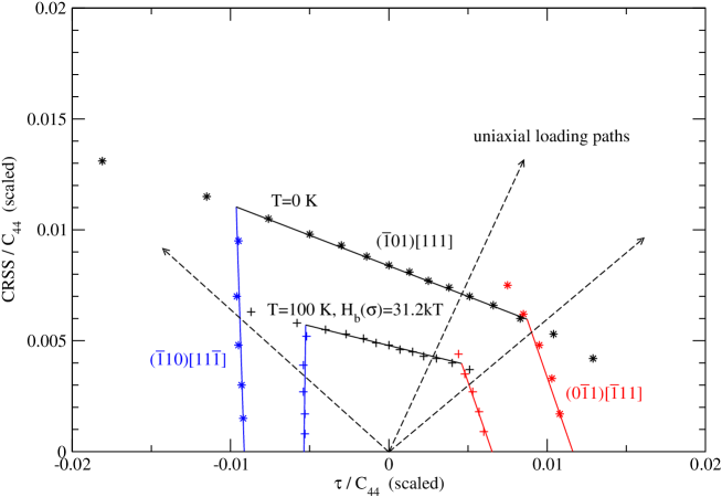
Figure 6.9: Combinations of shear stresses perpendicular and parallel to the slip direction that induce yielding of real single crystals of bcc molybdenum. The calculation is done solely using the temperature and strain rate dependent effective yield criterion in which $\tau^{*}_{cr}(T,\dot{\gamma})$ is obtained from Eq. 6.10.

The critical lines calculated using the above-mentioned procedure for $\chi=0$ are shown in Fig. 6.9 for $T=0~{}{\rm K}$ and $T=100~{}{\rm K}$; in the latter case, the activation enthalpy is chosen as $H_{b}(\sigma)=31.2kT$ which corresponds to the strain rate $\dot{\gamma}=8.6\times 10^{-4}~{}{\rm s}^{-1}$ used in the experiments of Hollang et al., (1997). In the limit of zero temperature, the critical lines correspond to those obtained earlier and plotted in Fig. 5.14. Due to the scaling of stresses that we introduced earlier in the calculation of the activation enthalpy, the stresses $\tau$ and $\sigma$ are now smaller than those in Fig. 5.14 and correspond to the magnitudes of stresses encountered in experiments. As one expects, at higher temperatures and/or lower strain rates $\dot{\gamma}$ (i.e. larger $q$), the stress to move the dislocation decreases and, therefore, the yield surface shrinks. This can be seen clearly in Fig. 6.9, where we plot the critical lines for the primary slip systems only.

It is important to note that more than two slip systems can be activated if the loading path intersects the yield polygon in Fig. 6.9 at one of its corners. This can be seen also in the $\pi$-plane projection of the yield surface in Fig. 4.6.

6.5 Comparisons with experiments

We have shown in Section 5.9 that the temperature dependence of the yield stress can be obtained theoretically by first calculating numerically the stress dependence of the activation enthalpy and then inverting it to recover the yield stress. This tedious process can now be replaced by using the derived formulas for $\sigma(T,\dot{\gamma})$ or $\tau^{*}_{cr}(T,\dot{\gamma})$ which, for uniaxial loading, only require a substitution of temperature, strain rate, angle $\chi$ of the MRSSP, and ratio $\eta=\tau/\sigma$.

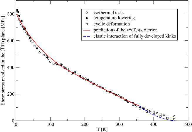
Figure 6.10: Temperature dependence of the yield stress, resolved as shear stress parallel to the $[111]$ slip direction and acting in the $(\bar{1}01)$ plane, for uniaxial tension along $[\bar{1}49]$ (curves). The symbols represent the experimental data of Hollang et al., (2001) obtained using three different techniques.

The tensile loading along the $[\bar{1}49]$ axis, used in the experiments of Hollang et al., (1997), corresponds to $\chi=0$, and the ratio of the two shear stresses to $\eta=0.51$. We use the experimental strain rate $\dot{\gamma}=8.6\times 10^{-4}~{}{\rm s}^{-1}$ (Hollang et al.,, 1997) and the previously estimated value $\dot{\gamma}_{0}=3\times 10^{10}~{}{\rm s}^{-1}$ to arrive at $q=\ln(\dot{\gamma}_{0}/\dot{\gamma})=31.2$. Substituting these parameters in Eq. 6.9 yields directly the temperature dependence of the yield stress $\sigma$ acting in the $(\bar{1}01)$ plane that is plotted in Fig. 6.10. One can observe a close agreement with experiment within a wide range of temperatures. At low temperatures, the theoretical prediction slightly departs from the experiment with the maximum deviation less than $20\ {\rm MPa}$. The same conclusion was reached previously by comparing the $\sigma-T$ dependence calculated numerically from the model of the dislocation bow-out (Section 5.2.2) and from the experiment, see Fig. 5.26.

Figure 6.11: Temperature dependence of the yield stress for two different strain rates $\dot{\gamma}$. The curves are calculated from Eq. 6.9 for low temperatures and from Eq. 6.11 for high temperatures. The symbols are the experimental data for two different strain rates from Hollang et al., (1997) and Hollang, (2001).

An important feature of $\tau^{*}_{cr}(T,\dot{\gamma})$, given by Eq. 6.10, and also the temperature dependence of the yield stress in Eq. 6.9 is their validity at different strain rates $\dot{\gamma}$. Since the parameter $q$ in the rate equation is inversely proportional to the plastic strain rate $\dot{\gamma}$, the temperature dependence of the yield stress decays to zero the more quickly the lower the value of $\dot{\gamma}$. In Fig. 6.11, we show the temperature dependence of the yield stress calculated for two different plastic strain rates, and their comparison with experimental data. At high temperatures, the yield stress is calculated from the approximation of the data obtained from the model of elastic interaction of fully developed kinks (6.11), whereas the low and intermediate temperatures are treated using Eq. 6.9. For any strain rate, the cross-over between the low-temperature and high-temperature approximation occurs at the yield stress equal to $115~{}{\rm MPa}$. This value is in good agreement with the experimental data plotted in Fig. 11 of Hollang et al., (1997), obtained for a wide range of plastic strain rates $\dot{\gamma}$, while the kink-pair formation theory presented thereafter predicts that this cross-over occurs at 180 MPa.

At high strain rates, both the theory and the experiments exhibit a marked change of slope at $\sigma=115~{}{\rm MPa}$ that can be attributed to the change of the shape of the dislocation in the activated state, particularly to the nucleation of two interacting kinks at high temperatures and to a continuous bow-out at low temperatures. In experiments, this change of slope completely vanishes at low strain rates and the linear regime at intermediate temperatures extends almost to the temperature at which the thermal component of the yield stress vanishes. The slight deviation of the theoretical calculations from experiments close to $115~{}{\rm MPa}$ does not constitute any major problem because the maximum error in $\sigma$ is only about $20~{}{\rm MPa}$.

6.6 Simplified “engineering” expressions for plastic flow

For practical calculations, it is always convenient to write the plastic strain rate $\dot{\gamma}$ as a simple function of temperature, stress, and other parameters. Due to the lack of detailed understanding of the microscopic nature of plastic deformation, these expressions were originally constructed purely phenomenologically and adjusted such that they correspond to experimental measurements. This approach has been adopted already by Kocks et al., (1975) who showed that the plastic strain rate can be approximated by the power law expression in which the Schmid stress is raised to a constant power that is obtained by fitting the experiment. Since none of these approximations involve the effect of non-glide stresses, which have been shown in preceding chapters to play an important role in bcc molybdenum, they are not applicable at low temperatures and high applied stresses.

Following our derivation of the temperature and strain rate dependent effective yield criterion, we can now derive the rate equation which will explicitly contain the effect of non-glide stresses. In principle, this can be done by considering the Arrhenius law $\dot{\gamma}=\dot{\gamma}_{0}\exp(-H_{b}(\sigma)/kT)$ in which the activation enthalpy, $H_{b}(\sigma)$, takes the form given by Eq. 6.6. For simplicity, consider a particular slip system $\alpha$ whose MRSSP is determined by the angle $\chi$, and $\eta$ is the ratio of the shear stress perpendicular to the shear stress parallel to the slip direction resolved in this MRSSP. Hence, the plastic strain rate in this system can be written as

$$\dot{\gamma}^{\alpha}=\dot{\gamma}_{0}\exp\left\{-\frac{2H_{k}}{kT}\left[1-a(\chi,\eta)\left(\frac{\sigma^{\alpha}}{C_{44}}\right)^{b(\chi,\eta)}\right]\right\}$$ (6.14)

if $\sigma^{\alpha}/C_{44}\leq 0.003$ and as

$$\dot{\gamma}^{\alpha}=\dot{\gamma}_{0}\exp\left\{-\frac{2H_{k}}{kT}\left[1-a^{\prime}(\chi,\eta)\exp\left(-\frac{b^{\prime}(\chi,\eta)}{\sigma^{\alpha}/C_{44}}\right)\right]\right\}$$ (6.15)

if $\sigma^{\alpha}/C_{44}\geq 0.003$. In these equations, $a,b,a^{\prime},b^{\prime}$ are quadratic functions of $\chi$ and $\eta$, and their coefficients obtained by fitting are summarized in Appendix D. The plastic strain rates have been calculated for nine characteristic combinations of $\chi$ and $\eta$ according to Eq. 6.14 and 6.15 and are plotted as symbols in Fig. 6.12. The slip system $\alpha$ considered for the calculations corresponds to $(\bar{1}01)[111]$ that is the dominant system for all chosen combination of $\chi$ and $\eta$. For convenience, we plot $\ln(\dot{\gamma}^{\alpha}/\dot{\gamma}_{0})$ as a function of $\ln(\tau^{*\alpha}/\tau^{*}_{cr})$, where the latter can be easily evaluated by noting that $\tau^{*\alpha}=\sigma^{\alpha}t(\chi,\eta)$; $t(\chi,\eta)$ was given earlier. Each cell in Fig. 6.12 corresponds to a fixed straight loading path, whose angle is determined by the stress ratio $\eta$ in the MRSSP characterized by the angle $\chi$, and contains three sets of data, for temperatures $T=10,50,450~{}{\rm K}$.

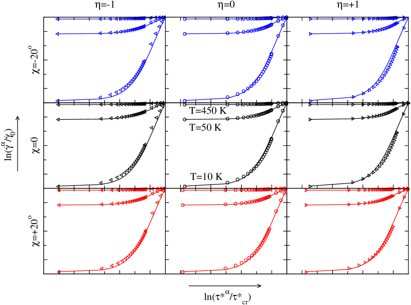
Figure 6.12: Stress dependence of the plastic strain rate obtained from the simplified formula (6.16) (curves) and its comparison with the data calculated from the original expressions (6.14) and (6.15) (symbols). Here, $\alpha$ corresponds to the most operative $(\bar{1}01)[111]$ system. Nine characteristic combinations of $\chi$ and $\eta$ are shown here; the ranges of values along the two axes are $\ln(\tau^{*\alpha}/\tau^{*}_{cr})\in\langle-8,0\rangle$, $\ln(\dot{\gamma}^{\alpha}/\dot{\gamma}_{0})\in\langle-1500,0\rangle$.

For engineering calculations, it is necessary to replace Eqs. 6.14 and 6.15 by one simple expression of $\dot{\gamma}^{\alpha}$ that could be written using primitive functions and still correctly accounts for the effect of non-glide stresses. In order to find this functional form, it is first helpful to look at the shape of the dependencies plotted in Fig. 6.12. It is clear that the approximate form of $\ln(\dot{\gamma}^{\alpha}/\dot{\gamma}_{0})$ for a given temperature $T$ must approach a constant at large negative $\ln(\tau^{*\alpha}/\tau^{*}_{cr})$ and vanish as $\ln(\tau^{\alpha*}/\tau^{*}_{cr})$ vanishes. The asymptotic character of $\ln(\dot{\gamma}^{\alpha}/\dot{\gamma}_{0})$ at negative $\ln(\tau^{*\alpha}/\tau^{*}_{cr})$ eliminates most of the primitive functions down to either $\tanh$ or $\arctan$ (Jeffrey,, 2000). Note, that both functions can approximate the data in Fig. 6.12 equally well and, therefore, there is no advantage of using one functional form over the other. In the following, we will utilize $\tanh$ only because it can be evaluated easily using exponentials. Hence, the data plotted in Fig. 6.12 can be closely approximated using the following functional form:

$$\dot{\gamma}^{\alpha}=\dot{\gamma}_{0}\exp\left\{-\frac{A}{kT}\left[B-\tanh\left(C\left(\ln\frac{\tau^{*\alpha}}{\tau^{*}_{cr}}+D\right)\right)\right]\right\}\ ,$$ (6.16)

where $k$ is the Boltzmann constant, $\dot{\gamma}_{0}=3\times 10^{10}~{}{\rm s}^{-1}$ is the pre-exponential term of the Arrhenius law in which the mobile dislocation density is a constant, and $A,B,C,D$ parameters that have to be adjusted such that the dependencies $\ln(\dot{\gamma}^{\alpha}/\dot{\gamma}_{0})-\ln(\tau^{*\alpha}/\tau^{*}_{cr})$, calculated from Eq. 6.16, match the data obtained from the two unsimplified expressions and plotted in Fig. 6.12 by symbols. At zero stress, as $\tau^{*\alpha}\rightarrow 0$, the product of $\tanh$ in Eq. 6.16 becomes -1 and the rate equation reduces to $\dot{\gamma}^{\alpha}=\dot{\gamma}_{0}\exp(-2H_{k}/kT)$, where $2H_{k}=A(B+1)$ is the energy of two isolated kinks. At large stresses, as $\tau^{*\alpha}\rightarrow\tau^{*}_{cr}$, the activation enthalpy vanishes and the rate equation has to read $\dot{\gamma}^{\alpha}=\dot{\gamma}_{0}$, which implies that the argument of the exponential of Eq. 6.16 is $A[B-\tanh(CD)]=0$. The four unknown parameters $A,B,C,D$ can now be determined by specifying $A$ and $C$ that control the height and slope of the $\tanh$ function in Eq. 6.16, after which $B$ and $D$ can be calculated from the two conditions above. For molybdenum, $\tau^{*}_{cr}=1014~{}{\rm MPa}$ and the best agreement with the data obtained from Eq. 6.14 and 6.15 is for the parameters listed in Tab. 6.1.

Table 6.1: Parameters $A,B,C,D$ for molybdenum used in Eqs. 6.16, 6.18 and 6.19.

$A$	$B$	$C$	$D$
0.90	0.41	0.60	0.73

.

The dependencies calculated from Eq. 6.16 with $A,B,C,D$ from the table above are plotted in Fig. 6.12 by solid curves. The total plastic strain rate can now be easily calculated by summing over the strain rates generated by each slip system $\alpha$, i.e.

$$\dot{\gamma}=\sum_{\alpha}\dot{\gamma}^{\alpha}\ .$$ (6.17)

Note, that the sum includes only the slip systems that contribute to the plastic flow, i.e. those for which $\tau^{*\alpha}>0$.

Eq. 6.16 also provides an elegant formula for the temperature and strain rate dependence of the yield stress that can be used instead of the original approximations (6.9) in which one would have to determine first the values of $a,b,a^{\prime},b^{\prime}$. Writing $\tau^{*\alpha}=\sigma^{\alpha}t(\chi,\eta)$, where $t(\chi,\eta)$ is the angular factor given earlier in Section 6.2, one obtains an expression for the yield stress, i.e. the shear stress $\sigma^{\alpha}$ parallel to the slip direction and applied in the MRSSP of the system $\alpha$:

$$\sigma^{\alpha}=\frac{\tau^{*}_{cr}}{t(\chi,\eta)}\exp\left\{-D+\frac{1}{C}\tanh^{-1}\left[B+\frac{kT}{A}\ln\frac{\dot{\gamma}^{\alpha}}{\dot{\gamma}_{0}}\right]\right\}\ ,$$ (6.18)

where the parameters $A,B,C,D$ are listed in Tab. 6.1. Since Eq. 6.18 is a simplified “engineering” expression of the temperature dependence of the yield stress, one should not expect that this formula will be capable of reproducing the experimental data as closely as its unsimplified version (6.9). To demonstrate this, we plot in Fig. 6.13 the temperature dependence of the yield stress calculated from Eq. 6.18 for loading in tension along the $[\bar{1}49]$ axis and its comparison with experimental data. This graph should be compared with Fig. 6.11 that shows the same dependence but calculated from the unsimplified Eq. 6.9 at low temperatures (high stresses) and from Eq. 6.11 at high temperatures (low stresses).

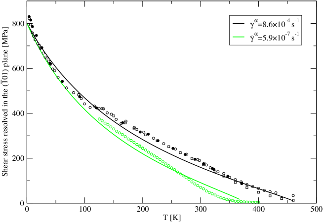
Figure 6.13: Temperature dependence of the yield stress calculated from the simplified expression (6.18) for loading in tension along $[\bar{1}49]$. Here, $\alpha$ is the most highly stressed $(\bar{1}01)[111]$ system. The symbols are the experimental data for two different strain rates from Hollang et al., (1997) and Hollang, (2001).

As expected, Eq. 6.18 correctly reproduces the overall trend of the experimental data but cannot resolve their details. This is the price that we pay for the demand to simplify the expressions for the plastic strain rate (6.14) and (6.15), and describe them by one analytical formula that is valid at all temperatures in which the plastic flow is controlled by thermally activated motion of screw dislocations. Nevertheless, the maximum deviation of the dependence predicted by Eq. 6.18 from the experiment is less than $30~{}{\rm MPa}$ and, therefore, Eqs. 6.16 and 6.18 represent reasonably accurate macroscopic representations of the plastic flow of single crystals of molybdenum. It is important to note that these expressions explicitly involve the effect of non-glide stresses that are included through $\tau^{*}$. Hence, a question arises naturally as to how different would the predictions of Eqs. 6.16 and 6.18 be if one considered the Schmid law instead of the full $\tau^{*}$ criterion. For a given $\chi$ and stress ratio $\eta$, this can be easily checked by setting $\tau^{*}$ equal to the Schmid stress, $\sigma\cos\chi$.

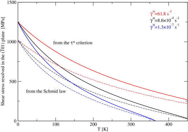
a) $\chi=0$, $\eta=\tau/\sigma=-1$

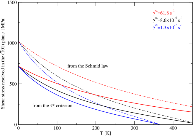
b) $\chi=0$, $\eta=\tau/\sigma=+1$

Figure 6.14: Temperature dependence of the yield stress calculated for three different strain rates $\dot{\gamma}^{\alpha}$ from Eq. 6.18. The solid lines are obtained by considering the $\tau^{*}$ criterion and the dashed lines are calculated from the Schmid law.

For illustration, we will consider two loading paths, specified by $\chi=0$ and $\eta=\{-1,+1\}$, and three different strain rates given by $q=\ln(\dot{\gamma}_{0}/\dot{\gamma}^{\alpha})=\{20,31.2,40\}$, where the middle value corresponds to the plastic strain rate $\dot{\gamma}=8.6\times 10^{-4}~{}{\rm s}^{-1}$ of the tensile experiments of Hollang et al., (1997). For this loading, we have already shown in Fig. 5.18 that the plastic flow is dominated by operation of the $(\bar{1}01)[111]$ system that we will denote as $\alpha$. The comparison of the dependencies calculated using the Schmid law, $\tau^{*\alpha}=\sigma^{\alpha}\cos\chi$, with those obtained from the full effective yield criterion, $\tau^{*\alpha}=\sigma^{\alpha}t(\chi,\eta)$, that involves all non-glide stresses is shown in Fig. 6.14 by the dashed and the solid curves, respectively. Obviously, the predictions of the Schmid law are independent of $\eta$ (and also of $\tau$), while the curves calculated from the $\tau^{*}$ criterion correctly reproduce the yield stress asymmetry for positive and negative shear stress perpendicular to the slip direction (see also Fig. 3.9a). At low temperatures and any plastic strain rate, the predictions made from the Schmid law deviate significantly from those calculated from the $\tau^{*}$ criterion, which is a clear manifestation of importance of non-glide stresses at low temperatures. This deviation gradually vanishes as the temperature is raised, which implies that the importance of non-glide stresses also diminishes with increasing temperature.

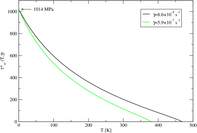
Figure 6.15: Variation of the effective yield stress with temperature, calculated from the simplified formula (6.19).

Eq. 6.18 also implies a convenient form of the temperature and strain rate dependent effective yield stress that is a simplified version of Eq. 6.10. At yield, $\tau_{cr}^{*}=\sigma^{\alpha}t(\chi,\eta)$, and, upon substituting $\sigma^{\alpha}$ from Eq. 6.18, this leads to

$$\tau^{*}_{cr}(T,\dot{\gamma})=\tau^{*}_{cr}(0)\exp\left\{-D+\frac{1}{C}\tanh^{-1}\left[B+\frac{kT}{A}\ln\frac{\dot{\gamma}}{\dot{\gamma}_{0}}\right]\right\}\ ,$$ (6.19)

where $\tau^{*}_{cr}(0)=1014~{}{\rm MPa}$ is the magnitude of the effective yield stress at zero temperature. The variation of $\tau^{*}_{cr}$ with temperature is shown in Fig. 6.15 for the two strain rates considered earlier. At a given temperature and strain rate, $\tau^{*}_{cr}(T,\dot{\gamma})$ represents the critical value of $\tau^{*\alpha}$ at which the slip system $\alpha$ becomes activated.

Finally, it is instructive to check the order of activity of individual slip systems at larger applied shear stress perpendicular to the slip direction. Without the loss of generality, we will consider loading by shear stress perpendicular ($\tau$) and parallel ($\sigma$) to the $[111]$ slip direction and choose the $(\bar{1}01)$ plane to be the MRSSP. We will consider two loading paths in the ${\rm CRSS}-\tau$ projection, given by the stress ratios $\eta=\pm 1.5$. For each of these loadings, we will identify the four slip systems $\alpha$ that can become operative, calculate the orientations of the MRSSPs, $\chi^{\alpha}$, in the zones of their slip directions, and determine the stress ratios $\eta^{\alpha}$ from the two shear stresses resolved in these MRSSPs. Eq. 6.18 then provides a critical shear stress $\sigma^{\alpha}$ that induces slip on each of the four slip systems $\alpha$. By resolving this stress back into the MRSSP of the $(\bar{1}01)[111]$ system, one arrives at the dependencies plotted in Fig. 6.16, where the loading paths are shown in the insets. At negative $\tau$, the plastic flow occurs by virtually simultaneous operation of the primary $(\bar{1}10)[11\bar{1}]$ and the secondary $(110)[\bar{1}11]$ system. These systems are identical to those predicted for $\eta=-1.5$ directly from the temperature and strain rate dependent effective yield criterion; the critical line for the former system is also shown in Fig. 6.9. At positive $\tau$, three slip systems are almost equally operative and the plastic flow occurs by simultaneous operation of $(0\bar{1}1)[\bar{1}11]$, $(\bar{1}01)[111]$ and $(0\bar{1}\bar{1})[11\bar{1}]$ systems. The operation of the two former systems is directly predicted for $\eta=+1.5$ from Fig. 6.9; the third system is not plotted in this figure because its critical line passes beyond the corner of the yield polygon.

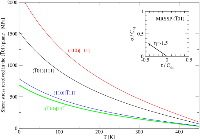
a) $\chi=0$, $\eta=\tau/\sigma=-1.5$ in the reference system $(\bar{1}01)[111]$

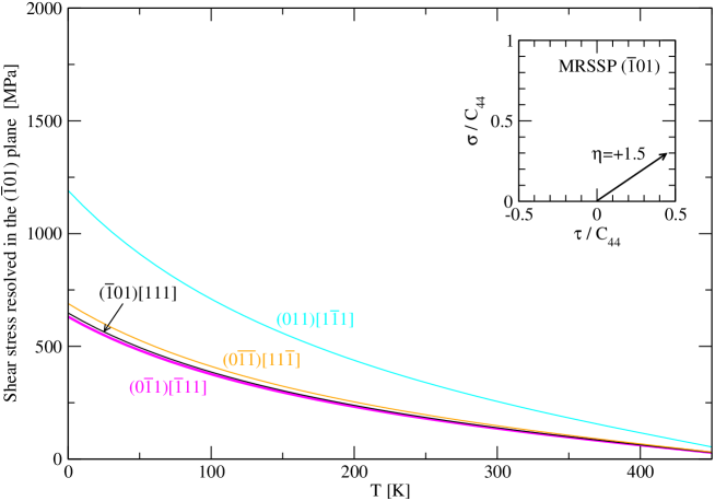
b) $\chi=0$, $\eta=\tau/\sigma=+1.5$ in the reference system $(\bar{1}01)[111]$

Figure 6.16: Temperature dependence of the yield stress for a fixed strain rate ($q=30$) and two loading paths for which the shear stress perpendicular to the slip direction is negative (a) and positive (b). The lowest curve corresponds to the primary slip system.

Based on the observed agreement between the theoretical prediction of the temperature dependence of the yield stress and experimental measurements, one may conclude that the “engineering” expressions (6.16), (6.18) and (6.19) correctly capture: (i) the effect of non-glide stresses, particularly twinning-antitwinning asymmetry and the effect of the shear stress perpendicular to the slip direction, (ii) decreasing role of non-glide stresses with increasing temperature, and (iii) the order of activation of individual slip systems. The approximate relations given in this section thus represent physically-based rules for plastic flow of single crystals of molybdenum in which the microscopic details of the motion of dislocations in each slip system $\alpha$ are condensed into the form of the effective stress $\tau^{*\alpha}$. Due to its relative simplicity, Eq. 6.16 provides for the first time a rate equation which explicitly accounts for the effect of non-glide stresses through physically based understanding of their effect on dislocation glide, and can thus be used in continuum finite-element calculations.

Chapter 7 Plastic flow of bcc tungsten

The significant problems we face cannot be solved at

the same level of thinking we were at when we created them.

Albert Einstein

In previous chapters we have shown in detail how the results of atomistic simulations of an isolated screw dislocation can be used to construct the effective yield criterion for molybdenum that correctly reproduces the effects of non-glide stresses in this material. Subsequently, this yield criterion was used to construct the Peierls potential and to calculate the stress dependence of the activation enthalpy, activation volume, and the temperature dependence of the yield stress. These dependencies were finally used to determine the temperature and strain rate dependent effective yield criterion that was shown to correctly reproduce the experimentally observed asymmetries of the yield stress.

In order to demonstrate that this approach can be used also for other bcc metals, we will now repeat the whole process and construct the plastic flow rules for tungsten. Because the details of this development have been explained thoroughly for molybdenum, we will focus only on the features that distinguish these two metals. The atomistic simulations presented in this chapter were performed using the screened BOP constructed specifically for tungsten (Mrovec et al.,, 2007). This potential correctly reproduces the elastic moduli, lattice parameter and the cohesive energy.

The crystallographic data and the elastic moduli for tungsten used in the forthcoming calculations are summarized below.

$\langle{100}\rangle$ lattice parameter	$a$	3.165
Shortest periodicity in $\{110\}\langle{112}\rangle$	$a_{0}$	2.584
Magnitude of the Burgers vector	$b$	2.741

Dimensions: [Å]

	$C_{11}$	5.224
Elastic moduli	$C_{12}$	2.044
	$C_{44}$	1.606
$\langle{111}\rangle$ shear modulus	$\mu$	1.595
Anisotropy factor		1.01

Dimensions: $C_{ij},\mu~{}[10^{5}~{}{\rm MPa}]$

7.1 $\gamma$-surface and the structure of the dislocation core

In Fig. 7.1, we show the unrelaxed and relaxed $\gamma$-surface calculated for bcc tungsten using the screened BOP. One can clearly see that there are no intermediate minima, and, therefore, no metastable stacking faults exist in tungsten. The unrelaxed $\gamma$-surface is in good agreement with the data obtained from full electron DFT simulations of Frederiksen and Jacobsen, (2003), which demonstrates the accuracy of the constructed potential.

Comparison of the fault energies corresponding to the displacements $b/3$ and $b/6$ (see Fig. 7.1) implies that $3\gamma(b/3)>6\gamma(b/6)$. Therefore, according to the criterion discussed in Section 3.1 screw dislocations in tungsten favor non-degenerate cores. Because the same type of dislocation core has been found in Section 3.1 for molybdenum, one may expect that the behavior of these two metals under stress will display common characteristics.

In subsequent 0 K atomistic studies of the effect of the applied stress on the screw dislocation, we adopted the same geometry of the simulation cell as used previously for molybdenum. The block was oriented such that the $z$-axis coincided with the dislocation line and thus the slip direction (i.e. the Burgers vector of the dislocation), $x$ axis coincided with the $[\bar{1}2\bar{1}]$ direction that is a trace of the $(\bar{1}01)$ plane on the $(111)$ plane, and $y$ was perpendicular to the $(\bar{1}01)$ plane. The block was effectively infinite along the dislocation line, which was achieved using periodic boundary conditions. In the $xy$ plane, perpendicular to the dislocation line, the block consisted of (see Fig. 3.3): (i) active region with atoms that move during the relaxation, and (ii) inert region that represents an infinitely large block in which the active region is embedded.

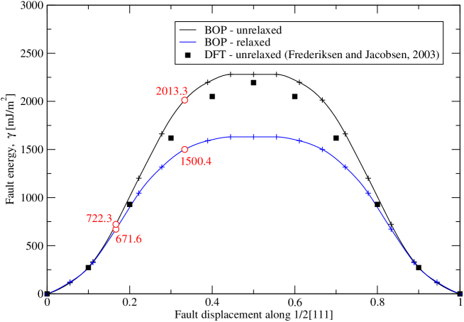
Figure 7.1: $\langle{111}\rangle$ cross-section of the $\{110\}$ $\gamma$-surface in tungsten calculated using the screened BOP and DFT.

Starting with a perfect single crystal, we inserted a $1/2[111]$ screw dislocation by displacing all atoms in the block according to the long-range strain field of the dislocation (Hirth and Lothe,, 1982). This configuration was subsequently relaxed using the BOP for tungsten. The differential displacement map showing the relaxed dislocation core is plotted in Fig. 7.2. In this projection, the circles again depict atoms in three successive $(111)$ layers separated by the distance $a/2\sqrt{3}$, where $a$ is the $\langle{100}\rangle$ lattice parameter. Each arrow corresponds to the mutual displacement of two atoms in the direction of the Burgers vector (i.e. perpendicular to the plane of the figure) and calculated relative to their distance in the perfect lattice.

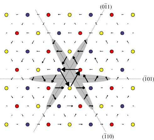
Figure 7.2: Structure of the $1/2[111]$ screw dislocation core calculated using the BOP for tungsten.

7.2 Behavior of dislocations under stress

In order to investigate the behavior of an isolated screw dislocation in tungsten under stress, we carried out a series of atomistic simulations at $0~{}{\rm K}$ using the BOP. From the original work of Ito and Vitek, (2001) and the Chapter 3 of this Thesis, we know that the motion of screw dislocations in molybdenum is affected only by shear stresses parallel and perpendicular to the slip direction. The latter exerts zero Peach-Koehler force on the dislocation and affects its motion only indirectly via modification of the structure of the dislocation core. On the other hand, the former stress exerts a nonzero Peach-Koehler force on the dislocation and can thus directly move it through the crystal when the applied stress reaches the Peierls stress. Owing to the fact that the dislocation core in tungsten is of the same type as that of molybdenum, one may assume that the plastic flow of tungsten is also affected only by the shear stresses parallel and perpendicular to the slip direction.

7.2.1 Loading by shear stress parallel to the slip direction

In this calculation we started with a completely relaxed block with a $1/2[111]$ screw dislocation in the middle, as shown in Fig. 7.2. The shear stress parallel to the slip direction, $\sigma$, was imposed on the block by applying to all atoms the anisotropic displacements corresponding to the stress tensor (3.1). To ensure a smooth convergence, the shear stress $\sigma$ was built up incrementally in steps of $0.001C_{44}$, where $C_{44}$ is the elastic modulus. In each loading step, the simulated block was fully relaxed before increasing $\sigma$. At stresses lower than the CRSS, the dislocation core transforms from its initially three-fold symmetric non-degenerate structure, to a less symmetric form. This transformation is purely elastic in that the block returns back into its original configuration when the stress is removed. Once the applied shear, $\sigma$, attains its critical value, the critical resolved shear stress (CRSS), the transformation is complete and the dislocation moves through the crystal.

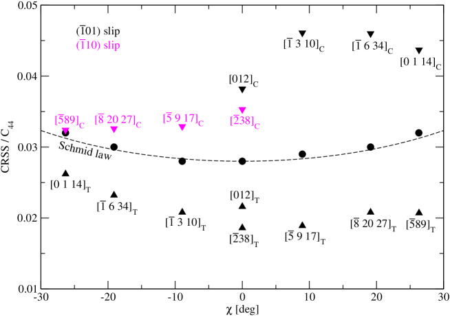
Figure 7.3: Orientation dependence of the CRSS for loading by pure shear stress parallel to the slip direction (circles) and for uniaxial loading (triangles). The subscripts _T and _C correspond to the loading in tension and compression, respectively.

In order to obtain the dependence of the CRSS on the orientation of the MRSSP, i.e. the angle $\chi$, we considered seven different angles $\chi$ spanning effectively the entire angular region $-30^{\circ}<\chi<+30^{\circ}$. The ${\rm CRSS}-\chi$ dependence obtained for loading by shear stress parallel to the slip direction is plotted in Fig. 7.3 with circles. For all orientations of the MRSSP, the dislocation moved by single slip on the $(\bar{1}01)$ plane. Importantly, the ${\rm CRSS}-\chi$ data follow the Schmid law, which means that no twinning-antitwinning asymmetry exists in tungsten. This is in contrast to molybdenum for which Fig. 3.6 reveals a strong orientation dependence of the CRSS for loading by pure shear stress parallel to the slip direction.

7.2.2 Loading in tension and compression

Superimposed in Fig. 7.3 are also the values of the CRSS calculated for loading in tension and compression (triangles). The loading axes were distributed uniformly throughout the entire interior of the stereographic triangle (Fig. 3.7) to cover a broad variety of possible orientations. For any loading axis, one can always find the orientation of the MRSSP in the zone of the $[111]$ slip direction that lies within $\pm 30^{\circ}$ from the $(\bar{1}01)$ plane. The shear stress parallel to the slip direction resolved in the MRSSP, characterized by the angle $\chi$, that moves the dislocation in tension/compression, is the CRSS that can be directly compared with the value calculated for the same angle $\chi$ when applying the pure shear stress parallel to the slip direction.

If, for a given $\chi$, the CRSS for tension/compression (triangles) were identical to those obtained for pure shear stress parallel to the slip direction (circles), we would conclude that only the shear stress parallel to the slip direction controls the plastic flow of tungsten. However, Fig. 7.3 clearly shows that this is not the case, and, therefore, the CRSS for slip must depend also on another stress component that is identified as the shear stress perpendicular to the slip direction.

7.2.3 Loading by shear stress perpendicular to the slip direction

Because the shear stress perpendicular to the slip direction cannot move the dislocation, the deformation induced by this stress in the crystal is purely elastic. This loading is applied by imposing the stress tensor (3.2) in steps of $0.005C_{44}$, as explained in Section 3.5.

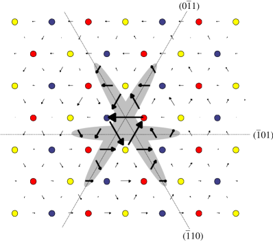
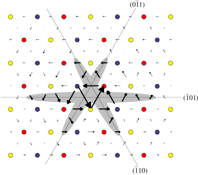
a) $\tau/C_{44}=-0.05$                                            b) $\tau/C_{44}=+0.05$

Figure 7.4: Structure of the relaxed dislocation core upon applying: (a) negative, and (b) positive shear stress perpendicular to the slip direction. The stress tensor (3.2) is applied in the coordinate system where the $y$-axis coincides with the normal of the $(\bar{1}01)$ plane.

For simplicity, we will discuss here only the case when the stress tensor is applied in the orientation for which the $y$-axis coincides with the normal of the $(\bar{1}01)$ plane, and the $z$-axis is parallel to the $[111]$ slip direction. The final structures of the dislocation core obtained by relaxing the simulated block at $\tau=\pm 0.05C_{44}$ are shown in Fig. 7.4. At negative $\tau$, the dislocation core constricts on the $(\bar{1}01)$ plane and extends on both $(0\bar{1}1)$ and $(\bar{1}10)$ planes. Due to the larger spreading of the core on the two low-stressed $\{110\}$ planes, the dislocation can move more easily in $(0\bar{1}1)$ and $(\bar{1}10)$ planes than in the most-highly stressed $(\bar{1}01)$ plane. On the other hand, at positive $\tau$, the dislocation core extends on the $(\bar{1}01)$ plane and constricts significantly on both $(0\bar{1}1)$ and $(\bar{1}10)$ planes. Since the core is now extended in the $(\bar{1}01)$ plane, one may expect that the subsequent loading by the shear stress parallel to the slip direction will move the dislocation in this plane.

In order to quantify the effect of the shear stress perpendicular to the slip direction on the magnitude of the CRSS for slip, we simulated a combined loading by these two stresses. The MRSSPs of applied loading considered in these simulations were identical to those involved in the studies of molybdenum, i.e. $(\bar{1}01)$ at $\chi=0$, $(\bar{6}15)$ and $(\bar{5}\bar{1}6)$ at $\chi=\pm 9^{\circ}$, $(\bar{3}12)$ and $(\bar{2}\bar{1}3)$ at $\chi=\pm 19^{\circ}$, and $(\bar{9}45)$ and $(\bar{5}\bar{4}9)$ at $\chi=\pm 26^{\circ}$. In each simulation, we first applied the shear stress perpendicular to the slip direction, $\tau$, according to the stress tensor (3.2). For a completely relaxed block at a given $\tau$, we superimposed the shear stress parallel to the slip direction, $\sigma$, by incrementally building up the stress tensor (3.1). When $\sigma$ reaches its critical value, identified as the CRSS for slip, the total applied stress tensor is given by Eq. 3.3 and the dislocation moves through the crystal. These simulations were carried out for several discrete values of $\tau$ that cover the usual magnitudes of stresses accessible in tension/compression tests. The dependence of the CRSS on $\tau$ for the above-mentioned orientations of the MRSSP is shown in Fig. 7.5. Recall that, if the Schmid law were valid in tungsten, the CRSS would be independent of $\tau$, and its magnitude would be equal to the Schmid stress, i.e. ${\rm CRSS}(\chi=0)=0.028C_{44}$. However, the obtained data clearly prove that the shear stress perpendicular to the slip direction strongly affects the magnitude of the CRSS for slip of screw dislocations in tungsten.

a) MRSSP $(\bar{1}01)$, $\chi=0$

b) MRSSP $(\bar{6}15)$, $\chi=+9^{\circ}$ and $(\bar{5}\bar{1}6)$, $\chi=-9^{\circ}$

c) MRSSP $(\bar{3}12)$, $\chi=+19^{\circ}$ and $(\bar{2}\bar{1}3)$, $\chi=-19^{\circ}$

d) MRSSP $(\bar{9}45)$, $\chi=+26^{\circ}$ and $(\bar{5}\bar{4}9)$, $\chi=-26^{\circ}$
Figure 7.5: Dependence of the CRSS on the shear stress perpendicular to the slip direction, $\tau$, for various orientations of the MRSSP.

At positive $\tau$, the CRSS decreases relative to $\tau=0$ and the slip always occurs on the most highly stressed $(\bar{1}01)$ plane. At small negative values of $\tau$, the dislocation glides on the most highly stressed $(\bar{1}01)$ plane. However, larger negative values of $\tau$ induce a significant core distortion, and the slip then occurs preferentially on either the $(0\bar{1}1)$ or the $(\bar{1}10)$ plane. The zig-zag slip on $\{112\}$ planes for $\chi=\pm 26^{\circ}$ and negative $\tau$ is caused by virtually equal shearing of the two adjacent $\{110\}$ planes. If we consider all possible slip systems, the Schmid factors corresponding to the $(0\bar{1}1)[111]$ and the $(\bar{1}10)[111]$ systems are typically only the fourth or the fifth highest among available slip systems, much lower than the most highly stressed $(\bar{1}01)[111]$ system. Similarly as in molybdenum, this gives rise to the anomalous slip which occurs as a consequence of the effect of the shear stress perpendicular to the slip direction.

It should be noted that, for positive $\tau$, the CRSS for antitwinning shear ($\chi>0$) is lower than the corresponding CRSS for the twinning shear ($\chi<0$). This is completely opposite to what we observed for molybdenum in Fig. 3.9a-d where, for positive $\tau$, the CRSS for antitwinning shear is always higher than that for the twinning shear.

Superimposed in Fig. 7.5a-d are also the results for several different orientations of uniaxial loadings. It is important to recognize that for such loadings the resolved $\tau$ is always positive for tension and negative for compression. One can observe a close agreement of the ${\rm CRSS}-\tau$ data calculated for tension/compression with the data for loading by a combination of the shear stresses perpendicular and parallel to the slip direction. This suggests that we have identified unambiguously all stress components that affect the plastic flow of single crystals of bcc tungsten. These stresses are: (i) shear stress perpendicular to the slip direction that merely changes the structure of the dislocation core, and (ii) shear stress parallel to the slip direction whose critical value (CRSS) determines the onset of the dislocation glide. The concomitant effect of these stress components on the onset of glide of an isolated $1/2[111]$ screw dislocation in tungsten is then given by the calculated ${\rm CRSS}-\tau$ dependencies. Unlike in molybdenum, however, in tungsten the CRSS for loading by pure shear stress parallel to the slip direction follows the Schmid law. Since there is no twinning-antitwinning asymmetry in tungsten, the only non-glide stress is the shear stress perpendicular to the slip direction.

7.3 Construction of the 0 K effective yield criterion

7.3.1 Fitting the atomistic results

The results of the atomistic studies, presented in the last section, can now be used to construct the effective yield criterion for tungsten. Similarly as in Section 4.2 for molybdenum, we will first determine the parameters $a_{1}$ and $\tau^{*}_{cr}$ in the restricted form of the $\tau^{*}$ criterion by fitting the ${\rm CRSS}-\chi$ dependence for loading by pure shear stress parallel to the slip direction, see Fig. 7.3. Keeping $a_{1}$ and $\tau^{*}_{cr}$ fixed, we subsequently obtain the coefficients $a_{2}$ and $a_{3}$ by fitting the ${\rm CRSS}-\tau$ dependencies for $\tau/C_{44}=\pm 0.01$. Again, we consider a priori only those atomistic data for which the slip occurs on the most highly stressed $(\bar{1}01)$ plane. If the criterion is constructed correctly, the change of the slip plane at larger negative $\tau$, shown in Fig. 7.5a-d, will be reproduced automatically.

Table 7.1: Coefficients of the effective yield criterion for tungsten determined by fitting the 0 K atomistic data.

$a_{1}$	$a_{2}$	$a_{3}$	$\tau^{*}_{cr}/C_{44}$
0	0.56	0.75	0.028

The coefficients of the $\tau^{*}$ criterion for tungsten, determined by fitting the atomistic results, are given in Tab. 7.1. Because the ${\rm CRSS}-\chi$ dependence obtained from loading by pure shear stress parallel to the slip direction follows the Schmid law, the parameter $a_{1}$ is obviously zero. This means that there is no twinning-antitwinning asymmetry in tungsten, which is corroborated already in Fig. 7.3. Both parameters $a_{2}$ and $a_{3}$ are now large, and this implies a strong dependence of $\tau^{*}$ on the shear stress perpendicular to the slip direction. The full form of the $\tau^{*}$ criterion is given by Eq. 4.3 and, in the case of tungsten, involves only three terms:

$$\tau^{*}=\sigma^{(\bar{1}01)}+a_{2}\tau^{(\bar{1}01)}+a_{3}\tau^{(0\bar{1}1)}\leq\tau_{cr}^{*}\ .$$ (7.1)

a) MRSSP $(\bar{1}01)$ at $\chi=0$

b) MRSSP $(\bar{2}\bar{1}3)$ at $\chi=-19^{\circ}$

c) MRSSP $(\bar{3}12)$ at $\chi=+19^{\circ}$
Figure 7.6: Critical lines from the $\tau^{*}$ criterion for tungsten calculated for three characteristic orientations of the MRSSP. Compare with Fig. 4.4 for molybdenum.

Similarly as in molybdenum, the $\tau^{*}$ criterion (7.1) with the coefficients from Tab. 7.1 can now be used to generalize the ${\rm CRSS}-\tau$ dependencies in Fig. 7.5 to real single crystals in which any $\{110\}\langle{111}\rangle$ system from Tab. 4.2 can be activated for slip by the applied loading. The details of these calculations are given in Section 4.3 and will not be repeated here. The results of these calculations are shown in Fig. 7.6, where the critical lines represent the loci of the loading states that cause the activation of individual slip systems. The inner envelope of these critical lines represents the projection of the yield surface.

For any loading, one can easily resolve the loading path in the ${\rm CRSS}-\tau$ plots in Fig. 7.6 corresponding to the actual MRSSP. If this path reaches the yield polygon at its edge, the plastic flow occurs by single slip on the system labeled in the figure. On the other hand, if it meets the yield polygon at its corner, two or more slip systems are activated for slip at once, and the plastic flow is then generated by simultaneous operation of these systems. These conclusions are very general and hold for any orientation of the MRSSP, as has been shown already in the case of molybdenum.

7.3.2 The 0 K yield surface

For simplicity, we will again discuss the $\pi$-plane projection of the yield surface that represents its cut by a plane whose normal is defined in the principal space as $\sigma_{1}=\sigma_{2}=\sigma_{3}$. If the plastic flow of tungsten were governed by the Schmid law, the $\pi$-plane projection of the yield surface would coincide with the Tresca’s regular hexagon. The actual shape of the yield surface is plotted in Fig. 7.7 and compared to the prediction of the Schmid law. Each edge of the polygon corresponds to operation of a particular slip system, while the corners mark a simultaneous slip on more than one system.

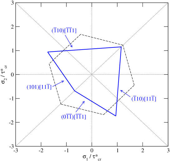
Figure 7.7: $\pi$-plane projection of the yield surface for tungsten calculated from the $\tau^{*}$ criterion (solid lines). The dashed Tresca hexagon corresponds to the purely Schmid behavior for which $a_{1}=a_{2}=a_{3}=0$.

Recall that, in the case of molybdenum, the $\pi$-plane projection of the yield surface was represented by an irregular hexagon, see Fig. 4.5. In the case of tungsten, the edges of the yield polygon in Fig. 7.7, corresponding to the $(\bar{1}10)[\bar{1}\bar{1}1]$ and the $(\bar{1}10)[11\bar{1}]$ systems, make an obtuse angle and this causes that the edges of the yield polygon in Fig. 4.5, corresponding to slip systems $(110)[1\bar{1}\bar{1}]$ and $(\bar{1}\bar{1}0)[1\bar{1}1]$, degenerate into a corner. Consequently, the $\pi$-plane projection of the yield surface in tungsten is represented by an irregular tetragon shown in Fig. 7.7.

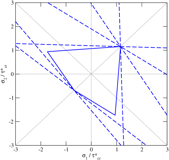
Figure 7.8: Yield polygon marking the onset of primary slip (solid line), and the critical lines corresponding to operation of non-primary slip systems (dashed lines).

Similarly as in molybdenum, multislip occurs when the loading path reaches one of the corners of the yield polygon. This is demonstrated in Fig. 7.8, where the dashed lines represent the loci of the loading states for which a given non-primary system becomes activated for slip. Clearly, only the loading directions for which $\sigma_{1}=\sigma_{2}$ lead to the onset of multislip on more than two systems. This means that, as the loading path reaches the yield surface close to any of these two corners, many slip systems will act simultaneously and significant strain bursts should be detectable in experiments.

7.3.3 The most operative slip systems in uniaxial loading

In Section 4.6, we used the 0 K effective yield criterion for molybdenum to predict the most operative slip systems under loading in tension and compression. We have shown in Fig. 4.7 that tensile loading along any direction always leads to the primary slip on the most-highly stressed $(\bar{1}01)[111]$ system, while for compression the nature of slip depends on the orientation of applied loading.

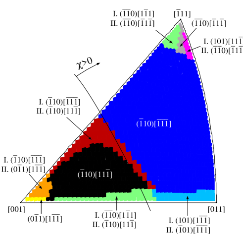
Figure 7.9: Primary slip systems for loading in compression determined from the $0~{}{\rm K}$ effective yield criterion for tungsten. Two slip systems operate simultaneously if the uniaxial yield stress of the secondary system (II.) is within 2% of that of the primary slip system (I.)

In tungsten, loading in tension along any axis in the stereographic triangle causes single slip on the most highly stressed $(\bar{1}01)[111]$ system, similarly as in molybdenum. In compression, the situation is much more complex and the choice of the primary system depends on the orientation of applied loading (see Fig. 7.9). For a large number of loading axes with MRSSPs corresponding to $\chi>0$, the most operative system with positive Schmid stress is $(\bar{1}10)[\bar{1}\bar{1}\bar{1}]$. On the other hand, for loading axes corresponding to the MRSSPs at $\chi<0$, the most operative system changes to $(\bar{1}10)[11\bar{1}]$. As the loading axis deviates toward one of the corners of the triangle, several slip systems become equally prominent, and the plastic flow proceeds by multislip on the corresponding systems. Interestingly, the $(\bar{1}01)[\bar{1}\bar{1}\bar{1}]$ system, which was most prominent in molybdenum, is now deferred to a tiny elongated region of multislip close to the $[011]$ corner of the triangle.

In Fig. 7.9, the Miller indices of the slip systems are written in such a way that the Schmid stress resolved in each system is always positive. This means that for loading in tension in the stereographic triangle $[001]-[011]-[\bar{1}11]$ (not shown in Fig. 7.9), only the slip systems 1 to 12 in Tab. 4.2 can become operative. Under loading in compression, the systems 1 to 12 are sheared in the opposite sense, the Schmid stress becomes negative, and, therefore, these systems cannot be activated for slip. Instead, one has to consider the conjugate systems 13 to 24 with opposite slip directions, which leads us to write $(\bar{1}01)[\bar{1}\bar{1}\bar{1}]$ and not $(\bar{1}01)[111]$.

7.3.4 Tension-compression yield stress asymmetry

The asymmetry between the yield stress in tension and compression will be again determined by the stress differential $\Delta\sigma_{t,c}$ that is defined by Eq. 4.8. For any loading axis, the uniaxial yield stress in tension and compression can be calculated directly from the constructed effective yield criterion. The distribution of $\Delta\sigma_{t,c}$ for tungsten is plotted in Fig. 7.10, where the symbols correspond to the same loading axes as in Fig. 7.3.

Figure 7.10: Variation of the stress differential (4.8) in tungsten with the orientation of the MRSSP for the loading axes from Fig. 7.3.

For any loading axis, we can determine the angle of the MRSSP, $\chi$, and resolve the shear stresses perpendicular and parallel to the slip direction. If only the shear stress parallel to the slip direction affected the plastic flow, $\Delta\sigma_{t,c}$ would be antisymmetric with respect to $\chi$. Since there is no twinning-antitwinning asymmetry in tungsten, this implies that there would be no asymmetry between the yield stresses in tension and compression, and $\Delta\sigma_{t,c}$ would be zero for any orientation of the loading axis. This is clearly not the case, as can be seen in Fig. 7.10, and $\Delta\sigma_{t,c}$ is thus nonzero due to the effect of the shear stress perpendicular to the slip direction. The effect of these non-glide stresses is so pronounced in tungsten that the region of positive $\Delta\sigma_{t,c}$, that emerged in molybdenum for orientations close to the $[011]$ corner (see Fig. 4.12a), is completely eliminated. Unfortunately, unlike for molybdenum, no comparison with experiments is currently possible for tungsten due to the lack of measurements performed on a given orientation in both tension and compression.

7.4 Construction of the Peierls potential

The Peierls potential for tungsten can be constructed by following the same procedure that was introduced in Section 5.4. Firstly, the mapping function $m(x,y)$ is written such that it reproduces the three-fold symmetry of the $[111]$ axis. Here, we will only consider the Peierls potential with flat saddle-points that was previously shown to reproduce correctly the experimentally measured temperature dependence of the yield stress for molybdenum. The modified mapping function that produces the Peierls barrier with flat maximum is obtained by perturbing all saddle-points of $m(x,y)$ by Eq. 5.57. In this function, we use the same parameters as for molybdenum, i.e. $\alpha=0.2$, $\beta=0.12$, and $r_{0}=a_{0}/3\sqrt{3}$, where $a_{0}$ is the periodicity of the lattice in the $\langle{112}\rangle$ direction in the $\{110\}$ plane. This function is applied to every saddle point of $m(x,y)$, which is emphasized by using the operator notation $\hat{f}m(x,y)$.

In order to evaluate the height of the Peierls potential, $\Delta V$, we consider loading by pure shear stress parallel to the slip direction in the $(\bar{1}01)$ plane. The actual MEP for an elementary jump of the dislocation between two adjacent minima on this plane is calculated using the NEB method and provides the Peierls barrier $V(\xi)$, where $\xi$ is the curved transition coordinate. The height of the Peierls potential, $\Delta V$, is obtained from the condition (5.41) in which the Peierls stress is now $\sigma_{P}=0.028C_{44}$. This condition is satisfied for

$$\Delta V=0.1369~{}{\rm eV}/{\rm\AA}\ .$$ (7.2)

The next step in the construction of the Peierls potential concerns the fitting of the function $K_{\sigma}(\chi)$ in Eq. 5.46, where $V_{\sigma}(\chi,\theta)$ represents the distortion of the three-fold symmetric basis of the potential by non-glide shear stresses parallel to the slip direction. Because the Schmid law now applies for loading by pure shear stress parallel to the slip direction, $K_{\sigma}(\chi)=0$, and, therefore, $V_{\sigma}(\chi,\theta)$ does not enter the formula (5.49) for the Peierls potential. Consequently, the Peierls potential for tungsten is not a function of the shear stress parallel to the slip direction.

Hence, we only need to consider the distortion of the Peierls potential by the shear stress perpendicular to the slip direction that is represented by the function $V_{\tau}(\chi,\theta)$, given by Eq. 5.50. To determine the parameters of the function $K_{\tau}(\chi)$, we again consider loading by $\tau=\pm 0.01C_{44}$ for which the dislocation moves on the $(\bar{1}01)$ plane, and, therefore, the Peierls stress in Eq. 5.41 is simply $\sigma_{P}={\rm CRSS}\cos\chi$. In this equation, the CRSS is determined from the $\tau^{*}$ criterion for tungsten, i.e. by means of Eq. 5.51 for parameters $a_{1}$, $a_{2}$, $a_{3}$ and $\tau^{*}_{cr}$ from Tab. 7.1. For a given angle $\chi$, the corresponding value of $K_{\tau}$ is obtained such that Eq. 5.41 is satisfied. This requirement yields

$$K_{\tau}(\chi)=-0.413-0.216\chi+0.782\chi^{2}\ .$$ (7.3)

In the case of tungsten, the Peierls potential (5.49) then reduces to

$$V(x,y)=[\Delta V+V_{\tau}(\chi,\theta)]\,\hat{f}m(x,y)\ ,$$ (7.4)

where $\Delta V$ is given by Eq. 7.2, and the functional form of $V_{\tau}(\chi,\theta)$ by Eq. 5.50 with $K_{\tau}(\chi)$ from Eq. 7.3.

For positive shear stress perpendicular to the slip direction, $\tau$, the potential develops a low-energy path along the $(\bar{1}01)$ plane and the dislocation thus preferentially moves on this plane. At negative $\tau$, this transition is suppressed by a large Peierls barrier and the dislocation moves instead by elementary steps on the $(0\bar{1}1)$ or the $(\bar{1}10)$ planes for which the Peierls barrier is lower.

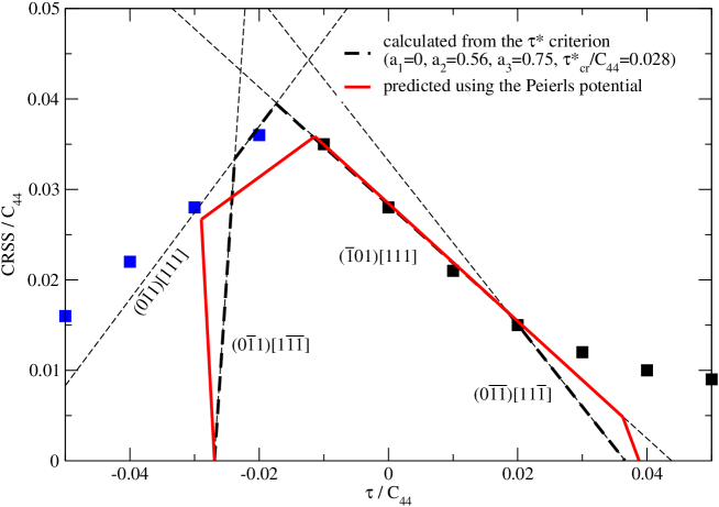
Figure 7.11: Critical lines calculated from the $\tau^{*}$ criterion and their comparison with the prediction of the constructed Peierls potential.

Similarly as in molybdenum, we can now employ the constructed Peierls potential and predict the dependence of the CRSS on $\tau$ directly from Eq. 5.41. As explained in detail in Section 5.5, this is achieved by considering a set of uniaxial loadings that correspond in the ${\rm CRSS}-\tau$ projection to straight loading paths emanating from the origin, with slopes $\eta=\tau/\sigma$. For a given loading, one can use the $\tau^{*}$ criterion to identify the four slip systems whose MRSSPs fall in $-30^{\circ}<\chi<+30^{\circ}$, and the Schmid stress is positive. For each of these systems, the CRSS is then calculated numerically from Eq. 5.41. This yields a set of four critical points along the given straight loading path in the ${\rm CRSS}-\tau$ projection that correspond to the onset of slip on these four systems. Repeating this calculation for a number of loading paths with different slopes $\eta$, and connecting the critical points for individual systems, generates the critical lines plotted as solid lines in Fig. 7.11. These lines correspond to the loci of the stress states that activate individual slip systems. Obviously, the critical line corresponding to the $(\bar{1}01)[111]$ system is in good agreement with the prediction of the $\tau^{*}$ criterion, because the data for the $(\bar{1}01)$ slip were used to fit the parameters in the function $K_{\tau}(\chi)$. However, the possibility of slip on other systems was not a priori considered, and, therefore, the agreement with the trend dictated for these systems by the $\tau^{*}$ criterion is a natural consequence of the constructed Peierls potential.

7.5 Thermally activated plastic flow of tungsten

7.5.1 Parameters entering the activation enthalpy

In order to incorporate the temperature and strain rate dependence of the yield stress, we will again first calculate the stress dependence of the activation enthalpy (for details, see Section 5.9). At low temperatures, this is given by the model of the dislocation bow-out (Section 5.2.2), while the high-temperature regime is treated by the model of elastic interaction of fully developed kinks (Section 5.2.3). Similarly as in molybdenum, we have to determine first the line tension of a straight screw dislocation such that the energy of two isolated kinks, $2H_{k}$, equals the experimentally deduced value. For tungsten, the measurements of Brunner and Glebovsky, (2000) imply $2H_{k}=2.06~{}{\rm eV}$, which is identical to the value obtained from the approximate formula, $2H_{k}\approx 0.1\mu b^{3}$, proposed by Conrad and Hayes, (1963). If Eq. 5.13 is to give the kink energy, the line tension of a straight screw dislocation has to be $V_{0}=p\mu b^{2}$ where $p=0.287$. With the $V_{0}$ fixed, the stress dependence of the activation enthalpy can be readily calculated from Eqs. 5.20 and 5.23.

The temperature and strain rate dependence of the yield stress can be included by means of the Arrhenius law $\dot{\gamma}=\dot{\gamma}_{0}\exp[-H(\sigma)/kT]$, where $H(\sigma)$ is the stress-dependent activation enthalpy calculated for a given orientation of applied loading. A straightforward way of determining $\dot{\gamma}_{0}$ is from experiments, by considering the temperature $T_{k}$ at which the thermal component of the yield stress vanishes. The activation enthalpy then reaches its maximum, $2H_{k}$, and the Arrhenius law gives $q\equiv\ln(\dot{\gamma}_{0}/\dot{\gamma})=2H_{k}/kT_{k}$, where $k$ is the Boltzmann constant. From the strain rate sensitivity experiments of Brunner and Glebovsky, (2000), performed at the nominal plastic strain rate $\dot{\gamma}=8.5\times 10^{-4}~{}{\rm s}^{-1}$, the temperature at which the thermal component of the yield stress vanishes is $T_{k}=760~{}{\rm K}$. Substituting these values into the equation above yields $\dot{\gamma}_{0}=3.7\times 10^{10}~{}{\rm s}^{-1}$ and $q=31.4$. Although this value is in good agreement with that obtained by fitting the experimental data of Brunner and Glebovsky, (2000) at temperatures close to $T_{k}$, their measurements also exhibit an abrupt change of $q$ at 600 K, from the value 31.4 (at $T>600~{}{\rm K}$) to 23.6 (at $T<600~{}{\rm K}$). If we recall that $q=\ln(\rho_{m}bv_{m}/\dot{\gamma})$ and assume that the velocity of mobile dislocations, $v_{m}$, is constant, this discontinuity implies a sudden change of $\rho_{m}$, the density of mobile dislocations, by three orders of magnitude. The temperature dependence of mobile dislocation density in tungsten is likely to exhibit a transient regime similar to that shown for intermetallic compounds Ni₃(Al,Hf) by Matterstock et al., (1999). In these materials, however, the increase of $\rho_{m}$ at the transient temperature is only by a factor of five. At present, the origin of the above-mentioned abrupt change of $\dot{\gamma}_{0}$ and $q$ in tungsten thus remains unresolved, and, therefore, one should consider the estimated $\dot{\gamma}_{0}$ only as an effective value.

7.5.2 Stress dependence of the activation enthalpy and volume

To allow further correlations with the experiments of Brunner and Glebovsky, (2000), performed under tension for an orientation close to the center of the stereographic triangle, we will consider tensile loading along the $[\bar{1}49]$ axis. The MRSSP of the most highly stressed $(\bar{1}01)[111]$ system is directly the $(\bar{1}01)$ plane ($\chi=0$), and the ratio of the shear stress perpendicular to the shear stress parallel to the slip direction, resolved in this plane, is $\eta=\tau/\sigma=0.51$. This is a key information that determines how the shape of the Peierls potential evolves during loading.

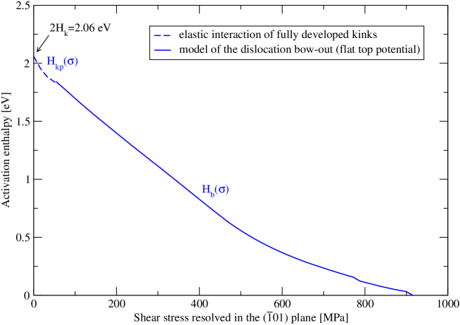
Figure 7.12: Stress dependence of the activation enthalpy for loading in tension along $[\bar{1}49]$. Here, $2H_{k}=2.06~{}{\rm eV}$ is the energy of two isolated kinks.

The activation enthalpy at high and low applied stresses can be obtained from the model of the dislocation bow-out (Section 5.2.2) and from the model of elastic interaction of fully developed kinks (Section 5.2.3), respectively. This calculation is the same as that performed in Section 5.6 for molybdenum. To ensure agreement between the theoretically calculated Peierls stress and the yield stress extrapolated from experimental data to 0 K, we have to scale all stresses by a factor of 3.7. This scaling accounts for interactions between dislocations that are not included in the atomistic simulations and may be also justified by the model presented in Appendix A. The obtained stress dependence of the activation enthalpy is shown in Fig. 7.12.

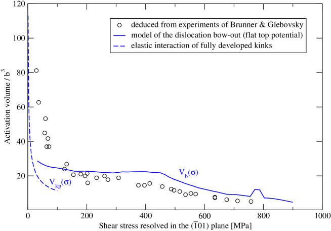
Figure 7.13: Stress dependence of the activation volume for loading in tension along $[\bar{1}49]$. The experimental data are deduced from Fig. 7 of Brunner and Glebovsky, (2000).

In Fig. 7.13, we plot the stress dependence of the activation volume that was deduced from the experimentally measured temperature dependence of the activation volume (Brunner and Glebovsky,, 2000) with help of the temperature dependence of the yield stress for tungsten by Hollang et al., (2001). The calculated activation volume, obtained as a negative derivative of the activation enthalpy with respect to stress, is plotted for the two models as full and dashed curves. The plateau at 400 K and the local maximum close to 800 K are both reminiscent of the same features shown for molybdenum in Fig. 5.25 and are manifestations of the flat maximum of the Peierls barrier.

7.5.3 Temperature dependence of the yield stress

The calculation of the temperature dependence of the yield stress was made for the experimental plastic strain rate $\dot{\gamma}=8.5\times 10^{-4}~{}{\rm s}^{-1}$. The low-temperature region of this dependence was calculated using the model of the dislocation bow-out, while high temperatures were treated within the model of elastic interaction of fully developed kinks. At all temperatures considered, the $(\bar{1}01)[111]$ system has the lowest activation enthalpy and thus the plastic deformation occurs by single slip on this system.

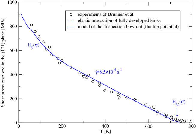
Figure 7.14: Calculated temperature dependence of the yield stress (strain rate $\dot{\gamma}=8.5\times 10^{-4}~{}{\rm s}^{-1}$) compared with experiments of Brunner and Glebovsky, (2000).

The theoretically calculated temperature dependence of the yield stress, obtained for the primary $(\bar{1}01)[111]$ slip system, corresponds to the curve in Fig. 7.14. It is important to emphasize, that this dependence has been calculated by considering that the dislocation moves at all temperatures by elementary jumps on the $(\bar{1}01)$ plane. The very good agreement of the theoretical predictions with experiments suggests that dislocations may indeed move by discrete $\{110\}$ jumps at all temperatures. Within this model, the change of slope of the dependence in Fig. 7.14 at 200 K is not caused by any transformation of the dislocation core, which has been raised as a possible explanation (Seeger,, 2004), but it is a manifestation of the flat maximum of the constructed Peierls barrier.

7.6 Temperature and strain rate dependent effective yield criterion

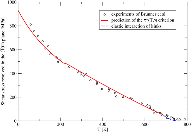
Figure 7.15: Temperature dependence of the yield stress calculated from the approximate expression (6.9) for loading in tension along $[\bar{1}49]$. The experimental data are from Brunner and Glebovsky, (2000).

For practical calculations, it is convenient to approximate the stress dependence of the activation enthalpy by a closed-form expression that replaces the tedious numerical calculations. This approximation has been thoroughly explained in Chapter 6. Firstly, we considered the loading by pure shear parallel to the slip direction that provided the restricted version of this approximation; see Section 6.1. Subsequently, the full form has been obtained by adding the effect of the shear stress perpendicular to the slip direction; see Section 6.2. The same approach can now be used for tungsten, which reduces merely to fitting the coefficients of the adjustable functions $a,b,a^{\prime},b^{\prime}$ to the data calculated for different $\chi$ and $\eta$ from the model of the dislocation bow-out. The functional forms of $H_{b}(\sigma)$, $\sigma(T,\dot{\gamma})$ and $\tau^{*}_{cr}(T,\dot{\gamma})$ all remain the same as those given by Eqs. 6.6, 6.9 and 6.10, respectively. For future reference, we list the coefficients entering the polynomials $a,b,a^{\prime},b^{\prime}$ for tungsten in Appendix D.

In order to verify that the constructed approximation reproduces correctly the experimental measurements, consider the loading in tension along $[\bar{1}49]$. The temperature dependence of the yield stress can then be obtained directly from Eq. 6.9, where the polynomials $a,b,a^{\prime},b^{\prime}$ are determined for $\chi=0$ and $\eta=0.51$. The obtained approximation of $\sigma(T)$ is plotted in Fig. 7.15 as the full curve. At high temperatures, the yield stress is determined by the elastic interaction of fully developed kinks (6.11) that corresponds in Fig. 7.15 to the dashed curve. One can see that the low-temperature approximation is in good agreement with the experiment at all temperatures for which the dislocation motion is thermally activated. Hence, for practical purposes, the model of elastic interaction of fully developed kinks is not needed, and one may safely use Eq. 6.9 at all temperatures up to $T_{k}=760~{}{\rm MPa}$.

7.7 Simplified “engineering” plastic flow rules

The simplified plastic flow rules that explicitly involve the effect of non-glide stresses can now be obtained in the same way as shown in Section 6.6 for molybdenum. We seek a reasonably accurate formula that replaces both the low and the high stress approximation of the plastic strain rate given by Eqs. 6.14 and 6.15. The functional form of this simplified expression is given by the same Eq. 6.16 that we have constructed originally for molybdenum. In this expression, the adjustable parameters for tungsten, determined by fitting, are given in Tab. 7.2, the critical yield stress $\tau^{*}_{cr}=1215~{}{\rm MPa}$ and the pre-exponential factor in the Arrhenius law $\dot{\gamma}_{0}=3.7\times 10^{10}~{}{\rm s}^{-1}$.

Table 7.2: Parameters $A,B,C,D$ for tungsten used in Eqs. 6.16, 6.18 and 6.19.

$A$	$B$	$C$	$D$
1.40	0.47	0.70	0.73

.

The Arrhenius law (6.16) with the parameters $A,B,C,D$ listed in Tab. 7.2 correctly reproduces the effect of non-glide stresses that enter $\dot{\gamma}$ via the magnitude of $\tau^{*}$. This can be demonstrated by calculating the temperature dependence of the yield stress from Eq. 6.18 that is shown for loading in tension along $[\bar{1}49]$ in Fig. 7.16. The overall agreement with the experimental data of Brunner and Glebovsky, (2000) is very satisfactory and proves that the simplified expressions given by Eqs. 6.16, 6.18 and 6.19 can indeed be used to describe the plastic flow of single crystals of tungsten at the temperatures for which the plastic flow is governed by the thermally activated motion of screw dislocations.

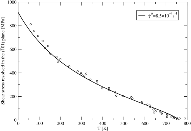
Figure 7.16: Temperature dependence of the yield stress for center-triangle orientation calculated from the engineering formula (6.18) and the parameters for tungsten listed in this section. The experimental data (circles) are due to Brunner and Glebovsky, (2000) and taken from Fig. 11.18 of Hollang et al., (2001).

Chapter 8 Conclusions

Perfection is achieved, not when there is nothing more to add,

but when there is nothing left to take away.

Antoine de Saint-Exupéry

Body-centered cubic refractory metals are crystallographically one of the simplest materials, and yet their plastic deformation exhibits a wealth of features that are not common in close-packed metals. The observed plastic deformation is always a result of many moving dislocations continuously produced by dislocation sources and a complex interplay of many dislocation processes. In contrast, atomic-level theoretical studies focus closely on the behavior of individual dislocations without invoking the complexity of the system, because it is generally recognized that $1/2\langle{111}\rangle$ screw dislocations govern the plastic deformation of bcc metals. This approach can provide essential information about the fundamental processes governing the plastic flow of bcc metals that can be later incorporated into mesoscopic and continuum models. Experimental observations have provided firm evidence that the plastic flow of bcc metals at low temperatures occurs by thermally activated motion of screw dislocations overcoming large lattice friction. However, no general framework has been introduced so far that would unify the microscopic behavior of isolated screw dislocations under stress with the macroscopic response determined by operation of many slip systems under a general loading.

The principal aim of this work has been to develop physically-based rules governing the plastic flow during macroscopic deformation of bcc transition metals that would explicitly involve the effects of temperature, strain rate, and the applied stress. This development is based on a multiscale model in which the fundamental microscopic information about the behavior of individual screw dislocations under stress is obtained from $0~{}{\rm K}$ atomistic studies. These simulations show that only the deviatoric component of the stress tensor plays a role in the dislocation glide, but, in contrast to the common wisdom, they reveal that both the shear stresses parallel and perpendicular to the slip direction affect the plastic flow in bcc metals. Although the latter stresses cannot directly move the dislocation, because they do not exert any Peach-Koehler force, they affect the structure of the dislocation core such that the glide of the dislocation occurs at lower or higher shear stress parallel to the slip direction, depending on the accompanying shear stress perpendicular to the slip direction. The atomic-level studies supply the dependence of the critical resolved shear stress (CRSS) at which the dislocation moves, i.e. the Peierls stress, on: (i) the orientation of the maximum resolved shear stress plane (MRSSP), and (ii) the shear stress perpendicular to the slip direction. These dependencies can be condensed into a $0~{}{\rm K}$ effective yield criterion that explicitly involves the effect of non-glide stresses, which are shear stresses parallel to the slip direction in a plane other than the slip plane and shear stresses perpendicular to the slip direction. For a given character of applied loading, this criterion can be used not only to determine the magnitude of the yield stress, but it also determines the order in which individual $\{110\}\langle{111}\rangle$ slip systems become activated for slip.

As the next step, the effective yield criterion, formulated on the basis of atomistic studies, was utilized to construct the Peierls potential that reflects the variation of the energy of a screw dislocation moving through the lattice. The Peierls potential is constructed as a two-dimensional function of the position of the intersection of the screw dislocation with the $\{111\}$ plane perpendicular to the dislocation line. It is based on a three-fold symmetric mapping function that reproduces the crystal symmetry. The transition path of the dislocation between two potential minima was determined using the Nudged Elastic Band method and the shape of the potential adjusted such that it yields the Peierls stress that is in agreement with the prediction of the $0~{}{\rm K}$ effective yield criterion. The novel concept introduced in this study is that the Peierls potential is a function of applied shear stresses, both parallel and perpendicular to the slip direction, which then reflects the calculated dependence of the Peierls stress on these applied stresses. The effects of temperature and strain rate are included through the mesoscopic model of formation and propagation of pairs of kinks. The rate of this process is given by an Arrhenius law with the activation enthalpy determined either from the model of the dislocation bow-out (high stresses and low temperatures) or the model of elastic interaction of fully developed kinks (low stresses and high temperatures). Owing to the stress dependence of the Peierls potential, the activation enthalpy is also a function of non-glide stresses as well as of the shear stress driving the dislocation motion. This is again a novel approach, in contrast with previous studies in which the activation enthalpy was always only a function of the shear stress driving the glide, i.e. the Schmid stress.

To allow comparisons with experiments in which many interacting dislocations give rise to the plastic flow, we proposed a mesoscopic model based on a collective motion of interacting parallel screw and mixed dislocations emitted from a Frank-Read source. This model suggests that the yield stress becomes by a factor of 2 to 3 lower than the Peierls stress of individual screw dislocations if one considers interactions between dislocations. This provides a physical explanation for the ubiquitous discrepancy between the theoretically calculated Peierls stresses and the measured yield stresses extrapolated to 0 K. Utilizing the above scaling of the yield stress, the calculated temperature dependence of the yield stress agrees very closely with experimental measurements. The stress dependence of the activation enthalpy is further approximated by an analytical formula that can be utilized to obtain a closed-form expression for the plastic strain rate and, most importantly, to formulate the temperature and strain rate dependent effective yield criterion. This criterion is shown to reproduce correctly the effect of non-glide stresses at low temperatures and their gradual decay with increasing temperature.

The multiscale model developed in this Thesis provides a plausible explanation of many features of the low-temperature plastic deformation of bcc metals, both at the level of individual dislocations and on the continuum level of crystal plasticity. In particular, atomistic simulations revealed a strong twinning-antitwinning asymmetry of the shear stress parallel to the slip direction in bcc molybdenum, but no such asymmetry has been found in bcc tungsten. However, in both metals, there is a strong effect of the shear stresses perpendicular to the slip direction that modify the structure of the dislocation core. If the core is constricted by these stresses in the most highly stressed $\{110\}$ plane in the zone of the slip direction, the slip typically proceeds on one of the lower-stressed $\{110\}$ planes. This may explain the origin of the so-called anomalous slip, i.e. deformation involving the slip system with a relatively low Schmid factor becomes the major deformation mode, which has been observed in many high-purity refractory bcc metals at low temperatures. This observation implies that the anomalous slip is induced by non-glide stresses that extend the core into one of the planes with a low Schmid factor and compress it in the plane of a high Schmid factor. Under uniaxial loading, the anomalous slip takes place only in compression. Very importantly, the experimentally observed slip of $1/2[111]$ dislocations on the $(0\bar{1}1)$ plane in tension should not be confused with the anomalous slip, because, for loading in tension, the Schmid factor for the $(0\bar{1}1)[111]$ system is comparable with that for the most highly stressed $(\bar{1}01)[111]$ system.

The proposed yield criterion reproduces successfully the asymmetry between the yield stress in tension and compression. In the case of bcc molybdenum, the yield criterion correctly predicts the experimental observations of Seeger and Hollang, (2000) that the yield stress in tension becomes higher than the yield stress in compression for orientations close to the $[011]$ corner of the stereographic triangle. It is important to emphasize that the constructed yield criterion predicts the tension-compression asymmetry, even when the MRSSP coincides exactly with the $(\bar{1}01)$ plane. This conclusion is in full agreement with the experimental observations of Seeger and Hollang, (2000). Finally, the effective yield criterion that follows from the proposed multiscale model, based on the behavior of individual screw dislocations at $0~{}{\rm K}$, is expressed as an analytical function of both temperature and plastic strain rate. This temperature and strain rate dependent effective yield criterion is shown to reproduce correctly the experimental measurements in the regime where the plastic deformation is governed by the nucleation and glide of screw dislocations.

Chapter 9 Future research

They are ill discoverers that think there is no land,

when they can see nothing but sea.

Sir Francis Bacon

Development of BOPs and plastic flow rules for other bcc metals

The multiscale approach to the development of the temperature and strain rate dependent yield criterion formulated in this Thesis for molybdenum and its subsequent testing on tungsten implies that this approach is likely to be applicable for any bcc metal. A similar development is planned in the future for tantalum, niobium and vanadium for which the construction of the BOP is currently under way. Moreover, the BOP for ferromagnetic bcc iron employing the Stoner model of band magnetism (Stoner,, 1938, 1939) is now under development at the University of Oxford and the UKAEA Culham Research Centre in the UK (Liu et al.,, 2005). These BOPs represent accurate empirical potentials that can be used to study the microscopic details of the plastic flow of bcc metals at low temperatures and will provide the fundamental information for the development of yield criteria for these materials.

Calculation of the Peierls potential using the Nudged Elastic Band method

The Peierls potential constructed in this Thesis is based on an assumed shape of the mapping function with adjustable parameters fitted such that it yields the Peierls stress that is in agreement with the $0~{}{\rm K}$ yield criterion constructed on the basis of the results of atomistic modeling of an isolated screw dislocation. This potential could, in principle, be calculated atomistically with the help of the Nudged Elastic Band method. In these calculations, the two fixed images would correspond to atomic blocks in which the dislocation is relaxed in two adjacent lattice sites. Each image along the elastic band is represented by $3N$ coordinates of the $N$ atoms in the simulated block. The final configuration corresponds to a chain of atomic blocks involving the dislocation in metastable positions. These positions and the differences between the energies of movable and fixed images then provide an energy barrier that has the same shape as the Peierls barrier and thus helps to formulate the Peierls potential more accurately.

Temperature dependence of the density of mobile dislocations

In the formulation of the macroscopic plastic flow rules, we have adopted the usual approximation that the density of mobile dislocations in each slip system does not vary significantly during loading and can thus be considered constant. This is a reasonable approximation at low temperatures, where the density of mobile dislocation increases mainly in the microyield regime but remains virtually constant at stresses close to the yield stress. At higher temperatures, the mobile dislocation density in intermetallic compound Ni₃Al typically exhibits a transient behavior (Matterstock et al.,, 1999) during which the density of dislocations rapidly increases. In order to verify the assumptions used in this work, it is important to investigate experimentally at what temperatures this transient occurs in refractory metals. If the transient temperature falls into the low-temperature regime, the rate equation may need a correction for the temperature dependence of the pre-exponential factor, $\dot{\gamma}_{0}$, in the Arrhenius law.

Mean field model of a group of interacting dislocations

On the macroscopic level, one of the most puzzling features is the change of shape of the temperature dependence of the yield stress measured for molybdenum (Hollang et al.,, 1997; Aono et al.,, 1983). This so-called “hump” (Seeger and Hollang,, 2000) has been asserted to be due to a hypothetical change of the mechanism of slip between the nucleation of kinks on $\{110\}$ planes at low temperatures and the formation of kinks on $\{112\}$ planes at intermediate and high temperatures. At present, atomistic simulation do not support this assertion because the slip of the dislocation on a $\{112\}$ plane can always be explained as a simultaneous operation of two or more $\{110\}\langle{111}\rangle$ systems. Provided that the dislocations move in groups, the above-mentioned shape irregularity could instead occur as a result of a “phase transition” between the low-temperature coherent dynamics in which the jumps of the dislocations are correlated, to the high-temperature incoherent dynamics in which the individual jumps are mutually uncorrelated events. This possibility should be studied in the future by investigating the steady-state behavior of a mean field model representing the chain of oscillators (dislocations) with long-range coupling, subjected to periodically varying substrate potential (i.e. the Peierls potential) and applied stress.

Appendix A Interactions between dislocations

In this Appendix, we propose a mesoscopic model that provides an explanation of the discrepancy between experimentally measured yield stresses of bcc metals at low temperatures and typical Peierls stresses determined by atomistic simulations of isolated screw dislocations. The model involves a Frank-Read type source emitting dislocations that become pure screws at a certain distance from the source and, owing to their high Peierls stress, control the operation of the source. However, due to the mutual interaction between emitted dislocations the group consisting of both non-screw and screw dislocations can move at an applied stress that is about a factor of two to three lower than the stress needed for the glide of individual screw dislocations.

A.1 Discrepancy between the Peierls stress and experimentally measured yield stresses

The vast majority of atomistic studies of the core structure and glide of $1/2\langle 111\rangle$ screw dislocations in bcc metals were carried out using molecular statics techniques and thus they correspond to 0 K. A problem encountered universally in all the calculations of the critical resolved shear stress (CRSS), i.e. the Peierls stress, at which the screw dislocation starts to glide, is that it is by a factor of two to three larger than the CRSS obtained by extrapolating experimental measurements to 0 K. The following are a few examples.

Basinski et al., (1981) measured the flow stress of potassium in the temperature range 1.5 K to 30 K and extrapolated to 0 K to get 0.002 to 0.003 where $\mu=(C_{11}-C_{12}+C_{44})/3$ is the $\{110\}\langle{111}\rangle$ shear modulus and $C_{11}$, $C_{12}$, $C_{44}$ are elastic moduli. Similar values were found by Pichl and Krystian, 1997b ; Pichl and Krystian, 1997a . The values of the CRSS when the MRSSP is a $\{110\}$ plane, calculated using a pair potential derived on the basis of the theory of weak pseudopotentials (Dagens et al.,, 1975), is 0.007 to 0.009 (Basinski et al.,, 1981; Duesbery,, 1984). More recently, Woodward and Rao, (2002) calculated the CRSS in molybdenum using the many-body potentials derived from the generalized pseudopotential theory (Moriarty,, 1990) and a DFT-based method. When the MRSSP was a $\{110\}$ plane, they found the CRSS to be between 0.018 and 0.020. A similar value of the CRSS, 0.019, was found in calculations employing the tight-binding based bond-order potential for molybdenum (Mrovec et al.,, 2004; Gröger and Vitek,, 2005). Experimental measurements of Hollang et al., (2001), extrapolated to 0 K, give for the CRSS in molybdenum 0.006. A similar problem was encountered by Wen and Ngan, (2000) who used the Embedded Atom Method (EAM) potential for iron and the Nudged Elastic Band method to analyze the activation enthalpies for kink-pair nucleation on screw dislocations. The calculated yield stress at 0 K was about 0.013 while the experimental values, reported by Aono et al., (1981) are 0.005 to 0.006. This variety of studies suggests that the reason for the discrepancy between calculated and measured CRSS cannot be sought in the inadequacy of the description of atomic interactions, which has often been raised as a possible explanation. In fact the ubiquitous higher value of the calculated CRSS, found independently of the description of atomic interactions, suggests that the origin of this discrepancy cannot be sought on the atomic scale of the motion of individual dislocations but rather on mesoscopic scale where a large number of elastically interacting dislocations glide at the same time. In this context it should be noticed that the only atomic level simulation that predicts the yield stress close to that measured experimentally considered a planar dislocation network of $1/2[111]$ and $1/2[\bar{1}\bar{1}1]$ screw dislocations with $[001]$ screw junctions (Bulatov and Cai,, 2002). Such a network moved in the $(\bar{1}10)$ plane at the stress about $50\%$ lower than the Peierls stress of an isolated dislocation.

A number of in-situ TEM observations of dislocation sources in bcc transition metals showed that in thin foils straight screw dislocations formed near the source and moved very slowly as a group, presumably due to a high Peierls stress (Vesely,, 1968; Louchet and Kubin,, 1975; Matsui and Kimura,, 1976; Saka et al.,, 1976; Takeuchi and Maeda,, 1977; Louchet et al.,, 1979; Louchet and Kubin,, 1979; Garrat-Reed and Taylor,, 1979; Louchet,, 2003). Hence they fully control the rate at which the source produces dislocations. In the foils used in TEM the applied stresses are very low but, owing to the same properties of screw dislocations, a similar control of the sources by sessile screw dislocations can be expected in the bulk at stresses leading to the macroscopic yielding. However, at higher stresses, dislocations move faster and do not become pure screws immediately after leaving the source but at a distance from the source. Indeed, even in situ observations at higher stresses do not show straight screw dislocations emanating directly from the sources (Vesely,, 2006).

In the following text, we propose a mesoscopic model involving a Frank-Read type source (Hirth and Lothe,, 1982; Hull and Bacon,, 2001) emitting dislocations of generally mixed character that become pure screw dislocations at a certain distance from the source and, owing to their high Peierls stress, still control its operation. However, there are a number of non-screw dislocations between the screws and the source, which can move easily. These dislocations exert a stress on the screw dislocations and these can then move at an applied CRSS that is about a factor of two to three lower than the CRSS needed for the glide of individual screw dislocations. This explains why the CRSS, obtained from the measurements of the yield and flow stresses extrapolated to 0 K, is usually about a factor of two to three lower than the Peierls stress of isolated screw dislocations.

A.2 Model of dislocation nucleation and motion

Let us consider a Frank-Read source (Hirth and Lothe,, 1982; Hull and Bacon,, 2001) that produces dislocations in a bcc metal. It emits, as always, dislocation loops that have a mixed character and expand easily away from the source since their Peierls stress is low. However, at a certain distance from the source, a significant part of the expanding loop attains the screw orientation and becomes much more difficult to move owing to the very high Peierls stress. The rest of the loop, having a mixed character, continues to move which leads to further extension of the screw segments. As a result, the source becomes surrounded by arrays of slowly moving screw dislocations, as depicted schematically in Fig. A.1. Further operation of the source is hindered by their back stress and effectively controlled by the ability of the screw dislocations to glide.

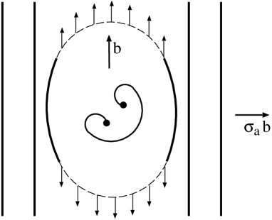
Figure A.1: Schematic operation of a dislocation source in bcc metals. When the curved non-screw segments migrate away, they leave behind a new pair of screw dislocations.

The operation of the source is driven by the applied stress, $\sigma_{a}$, which acts by the Peach-Koehler force (Hirth and Lothe,, 1982) $\sigma_{a}b$ per unit length of the dislocation that bows out. This dislocation obviously has a mixed character. Let us consider now that there are $N_{s}$ screw dislocations at distances $x_{i}$ from the source and $N_{m}$ dislocations, generally of mixed character, positioned between the source and the screw dislocations. We approximate the latter as straight lines of the same orientation as the screws, positioned at distances $y_{k}$ from the source, but with a negligible Peierls stress when compared with that of the screws. In the framework of the isotropic elastic theory of dislocations the condition for the source to operate is then

$$\sigma_{a}b\geq\frac{\tau}{R}+\frac{\mu b^{2}}{2\pi\alpha}\sum_{i=1}^{N_{s}}\frac{1}{x_{i}}+\frac{\mu b^{2}}{2\pi\beta}\sum_{k=1}^{N_{m}}\frac{1}{y_{k}}\ ,$$ (A.1)

where $\tau$ is the line tension of the emitted dislocations, $b$ their Burgers vector, $R$ the half-length of the source, $\mu$ the shear modulus and $\alpha$, $\beta$ constants of the order of unity. The first term is the force arising from the line tension that pulls the nucleating loop back and the second and third terms are forces produced by the stress fields of screw and non-screw dislocations, respectively, present ahead of and/or behind the source. In the following we neglect the interaction between dislocations ahead and behind the source as they are far apart. Moreover, the dislocation sources are frequently single-ended (Hull and Bacon,, 2001). Hence we analyze only dislocations ahead of the source, i.e. dislocations towards which the source bows out.

It should be noted here that the screw dislocations in the array ahead of the source are not pressed against any obstacle and thus they do not form a pile-up. Within the approximations defined above, the $i$th screw dislocation will move provided

$$\sigma_{a}+\frac{\mu b}{2\pi\alpha}\mathop{\sum_{j=1}^{N_{s}}}_{j\not=i}\frac{1}{x_{i}-x_{j}}+\frac{\mu b}{2\pi\beta}\sum_{k=1}^{N_{m}}\frac{1}{x_{i}-y_{k}}+\frac{\mu b}{2\pi\beta}\frac{1}{x_{i}}\geq\sigma_{P}\ ,$$ (A.2)

where $\sigma_{P}$ is the Peierls stress of screw dislocations. The second and third terms are stresses arising from screw and non-screw dislocations, respectively, which have been produced by the source, and the fourth term is the stress arising from the dislocation associated with the source that is also treated as a straight line of the same type as all the other mixed dislocations. Since the Peierls stress of non-screw dislocations is negligible, the $l$th non-screw dislocation can move provided

$$\sigma_{a}+\frac{\mu b}{2\pi\alpha}\sum_{j=1}^{N_{s}}\frac{1}{y_{l}-x_{j}}+\frac{\mu b}{2\pi\beta}\mathop{\sum_{k=1}^{N_{m}}}_{k\not=l}\frac{1}{y_{l}-y_{k}}+\frac{\mu b}{2\pi\beta}\frac{1}{y_{l}}\geq 0\ .$$ (A.3)

Now, the question asked is how large stress, $\sigma_{a}$, needs to be applied so that the screw dislocations can move so far away from the source that they either reach a surface or encounter dislocations of opposite sign from another source and annihilate. In both cases the source then keeps producing new dislocations indefinitely. In the former case these dislocations keep vanishing at the surface and the latter case leads to the propagation of slip through the sample. In order to investigate the problem formulated above we performed the following self-consistent simulations that were carried out for certain fixed values of the Peierls stress, $\sigma_{P}$, and applied stress $\sigma_{a}$. First we choose a half-length of the source, $R$, and a distance from the source, $y_{max}$, beyond which the expanding loop always attains the screw character. The first mixed dislocation, emitted by the source, becomes screw when reaching the distance $y_{max}$ from the source and then moves to a distance $x_{1}$, determined by Eq. A.2. Provided that the source can operate, i.e. the inequality (A.1) is satisfied, another dislocation is emitted from the source. The position of this dislocation is determined by Eq. A.3 if it does not reach $y_{max}$ and by Eq. A.2 if it does. Subsequently, the position of the first dislocation, $x_{1}$, is updated to satisfy Eq. A.2, which allows also the second dislocation to move. In this way a new position of the first dislocation, $x_{1}$, and the position of the second dislocation, either $y_{1}$ if smaller than $y_{max}$ or $x_{2}$ if larger than $y_{max}$, are found self-consistently. This self-consistent process is then repeated for the third, fourth, etc., dislocations until the source cannot emit a new dislocation, i.e. when the inequality (A.1) cannot be satisfied. The result of this calculation is the number of screw dislocations, $N_{s}$, and mixed dislocations, $N_{m}$, as well as their positions ahead of the source when it becomes blocked by the back-stress from all the emitted dislocations. The first screw dislocation is then at a position $x_{1}=x_{max}$ and further operation of the source can proceed only if this screw dislocation is removed. This can occur if it is either attracted to a free surface or annihilates after encountering the dislocation of opposite sign produced by another source. The source can then continue operating in a steady-state manner producing a large number of dislocations that mediate the macroscopic plastic flow.

A.3 Simulation of an array of interacting dislocations

In the following numerical simulations, the applied stress $\sigma_{a}$ was set equal to $0.3\sigma_{P}$ and $0.5\sigma_{P}$, respectively, in order to investigate whether the source can operate at stress levels corresponding to experimental yield stresses extrapolated to 0 K. Three values of the Peierls stress, $\sigma_{P}$, have been considered that fall into the range found in atomistic studies of transition metals (Woodward and Rao,, 2002; Mrovec et al.,, 2004; Gröger and Vitek,, 2005; Wen and Ngan,, 2000), namely $0.01\mu$, $0.02\mu$, and $0.03\mu$. Three different positions at which mixed dislocations transform into screw ones have been considered, namely $y_{max}/b=500,1000,$ and 2000. The dependence on the size of the source, $R$, was also investigated. However, this dependence is very weak since $R$ enters only through the line tension term in Eq. A.1 and this is always small compared to the terms arising from the back-stress of emitted dislocations. Hence, without the loss of generality, we set $R=y_{max}$. The values of parameters $\alpha$ and $\beta$, entering equations (A.1) to (A.3) have all been set to one and the usual approximation for the line tension, $\tau=\mu b^{2}/2$ (Hirth and Lothe,, 1982) was adopted.

Figure A.2: Positions of mixed (open circles) and screw (full circles) dislocations when the source is blocked are shown on the horizontal axis for the case $\sigma_{a}/\sigma_{P}=0.5$, $\sigma_{P}/\mu=0.02$, and $y_{max}/b=500$. In this case, $x_{max}/y_{max}=1.8$ (see Tab. A.1). The stress evaluated at the positions of these dislocations is shown on the vertical axis.

Results of such simulation are presented in detail for $\sigma_{a}=0.5\sigma_{P}$, $\sigma_{P}=0.02\mu$ and $y_{max}=500b$ in Fig. A.2, where positions of the dislocations ahead of the source and stresses acting on them are shown. In this case $x_{max}/y_{max}=1.8$. It should be noted that the stress exerted on the majority of screw dislocations is practically equal to the Peierls stress. The distances $x_{max}$ found for the above-mentioned two values of $\sigma_{a}/\sigma_{P}$, three values of $\sigma_{P}/\mu$ and three values of $y_{max}/b$, are summarized in Tab. A.1. These results suggest that, for a given applied stress, the ratio is almost constant, independent of $y_{max}$, and only weakly dependent on the magnitude of the Peierls stress $\sigma_{P}$. At $\sigma_{a}/\sigma_{P}=0.3$, most of the dislocations are mixed and $x_{max}/y_{max}\approx 1.3$. With increasing stress, more emitted dislocations become screw and, at $\sigma_{a}/\sigma_{P}=0.5$, $x_{max}/y_{max}\approx 2$, which implies that the numbers of mixed and screw dislocations ahead of the source are very similar. Very importantly, the stress exerted on most of the screw dislocations is practically equal to the Peierls stress..

Table A.1: The distance which the leading screw dislocation advances from the source, $x_{max}$, as a function of the distance $y_{max}$ from the source at which dislocations become screw, applied stress $\sigma_{a}/\sigma_{P}$, and the Peierls stress of the screw dislocations $\sigma_{P}/\mu$.

		$y_{max}/b$
		500	1000	2000
$\sigma_{a}/\sigma_{P}=0.3$
	$\sigma_{P}/\mu=0.01$	1.0	1.1	1.2
$x_{max}/y_{max}$	$\sigma_{P}/\mu=0.02$	1.2	1.3	1.3
	$\sigma_{P}/\mu=0.03$	1.2	1.2	1.2
$\sigma_{a}/\sigma_{P}=0.5$
	$\sigma_{P}/\mu=0.01$	1.6	1.8	2.0
$x_{max}/y_{max}$	$\sigma_{P}/\mu=0.02$	1.8	2.0	2.0
	$\sigma_{P}/\mu=0.03$	1.9	2.0	2.0

A.4 Discussion

The mesoscopic model presented in this appendix suggests that in bcc metals the dislocation generation may be sustained at an applied stress that is by a factor of two or three smaller than the Peierls stress of $1/2\langle{111}\rangle$ screw dislocations that control the plastic deformation of these metals. The distinguishing characteristic of this model is that it does not consider the glide of a single screw dislocation but movement of a large group of dislocations produced by a Frank-Read type source. In general, this source produces dislocation loops of mixed character that transform into pure screws at a distance $y_{max}$ from the source. Hence, the group of dislocations consists of screw dislocations at distances larger than $y_{max}$ and non-screw dislocations near the source. It is then the combination of the applied stress with the stress produced by the dislocations in the group that acts on the screw dislocations and is practically equal to their Peierls stress. However, once the leading screw dislocation reaches the distance $x_{max}$ from the source the operation of the source is blocked. Nonetheless, it can continue operating if a dislocation of opposite sign, originating from another source, annihilates the leading screw dislocation, as shown in Fig. A.3. This requires that the average separation of sources be about $2x_{max}$. Since the pinning points of the sources for a given slip system are produced by intersections with dislocations in other slip systems, their separation is related to the dislocation density in these systems. For example, in a deformed molybdenum crystal this density is of the order of $10^{12}\,{\rm m}^{-2}$ (Kaspar et al.,, 2000) which implies separation of dislocations between $3000b$ and $4000b$, for the lattice parameter of Mo equal to $3.15\,{\rm\AA}$. These values are in the range of $2x_{max}$ for applied stresses that are between one-third and one-half of the atomistically calculated Peierls stress for the sources of the size compatible with the above-mentioned density of dislocations.

The implication of the present study is that the values of the Peierls stress of screw dislocations in bcc metals found in atomistic studies cannot be compared directly with the critical resolved shear stresses obtained by extrapolating experimental measurements to 0 K. The experiments do not determine the stress needed for the glide of individual screw dislocations but, instead, the stress needed for the operation of sources that are hindered by the sessile screw dislocations. These sources can operate at stresses lower than the Peierls stress owing to the collective motion of screw and mixed dislocations produced by them, as described earlier.

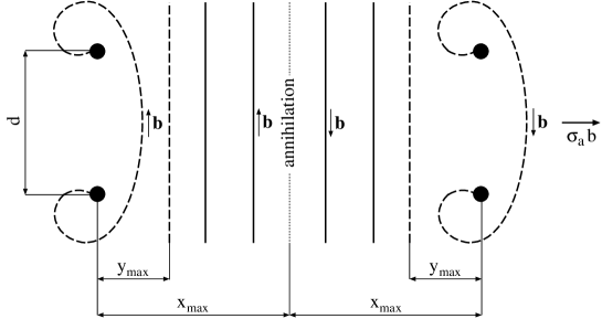
Figure A.3: Schematic illustration of the operation of two dislocation sources. Dislocations of opposite Burgers vectors mutually annihilate when reaching the distance $x_{max}$ from the source. The circles are pinning points of the source, dashed and solid lines are mixed and screw dislocations, respectively. The pinning points are commonly forest dislocations intersecting the slip plane and their density is approximately $\rho=4/2dx_{max}$, where $d$ is the size of the source.

The model presented here in no way implies a need for some more sophisticated and less comprehensive simulation schemes. On the contrary, single dislocation studies provide a great insight and understanding of the onset of plastic deformation in these materials. For the comparison with experiments, the theoretically calculated Peierls stresses may be scaled down by a factor of two or three to meet the experimental data. However, in the framework of the proposed model, this scaling should always be understood as a posteriori accounting for interactions between dislocations that are not included in the atomistic model.

Appendix B Euler angles and transformations between slip systems

Consider two Cartesian coordinate systems $\alpha_{1}$ and $\alpha_{2}$. The transformation from the former to the latter system generally requires knowledge of the full ($3\times 3$) transformation matrix. However, according to the Euler’s rotation theorem, the same transformation can be conveniently described using only three angles that define rotations about the three coordinate axes. The choice of the Euler angles is not unique; the so-called $x$-convention, or the $zxz$ rotation, is one of the most common schemes. In this convention, the rotation from system $\alpha_{1}$ to $\alpha_{2}$ is given by Euler angles ($\phi$,$\theta$,$\psi$), where the first rotation is by an angle $\phi$ about the $z$-axis, the second by an angle $\theta$ about the $x$-axis, and the third by an angle $\psi$ again about the $z$-axis. The transformation matrix reads

$$\boldsymbol{A}=\left[\begin{array}[]{ccc}a_{11}&a_{12}&a_{13}\\ a_{21}&a_{22}&a_{23}\\ a_{31}&a_{32}&a_{33}\end{array}\right]\ ,$$ (B.1)

where the components $a_{ij}$ are defined in terms of the given Euler angles $\phi$, $\theta$ and $\psi$ as follows:

$$a_{11} = \cos\psi\cos\phi-\cos\theta\sin\phi\sin\psi$$

$$a_{12} = \cos\psi\sin\phi+\cos\theta\cos\phi\sin\psi$$

$$a_{13} = \sin\psi\sin\theta$$

$$a_{21} = -\sin\psi\cos\phi-\cos\theta\sin\phi\cos\psi$$

$$a_{22} = -\sin\psi\sin\phi+\cos\theta\cos\phi\cos\psi$$ (B.2)

$$a_{23} = \cos\psi\sin\theta$$

$$a_{31} = \sin\theta\sin\phi$$

$$a_{32} = -\sin\theta\cos\phi$$

$$a_{33} = \cos\theta$$

In the following, we will show how the concept of Euler angles can be used to obtain the ${\rm CRSS}-\tau$ dependencies for real single crystals that correspond to other reference systems than $(\bar{1}01)[111]$. The fact that all $\{110\}\langle{111}\rangle$ systems in bcc crystals are mutually equivalent allowed us to formulate the 0 K effective yield criterion (4.6) such that it holds for all slip systems. As a result, we arrived at a series of critical lines in the ${\rm CRSS}-\tau$ projection of each MRSSP, defining the onset of slip on the corresponding slip systems. For example, the obtained dependence for the MRSSP $(\bar{1}01)$ corresponding to $\chi=0$ is shown in Fig. B.1a, where the dashed lines are loci of critical loadings for which the slip on individual systems takes place.

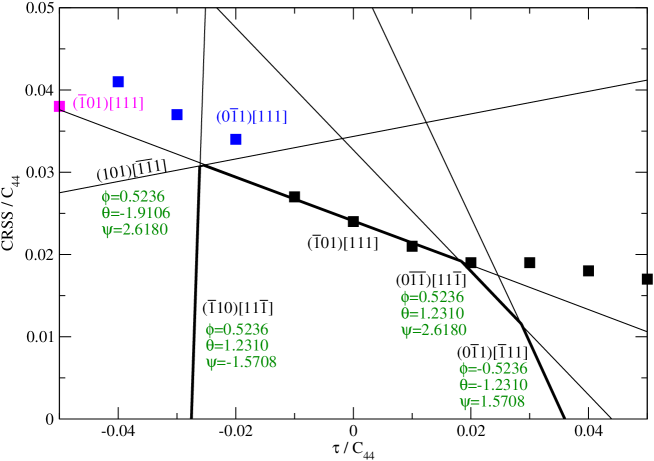
a) reference system $(\bar{1}01)[111]$

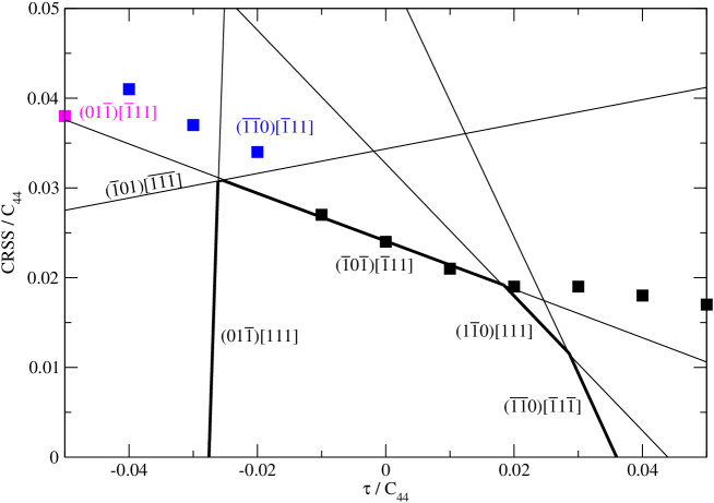
b) reference system $(\bar{1}0\bar{1})[\bar{1}11]$

Figure B.1: Projection of the MRSSP at $\chi=0$ for two different reference systems in which the angle of $\chi$ is measured. The numbers below the designations of slip systems in a) give the Euler angles between an individual system and the corresponding reference system.

Since all 24 slip systems in Tab. 4.2 are physically equivalent, the ${\rm CRSS}-\tau$ plot in Fig. B.1a, correspoding to the reference system $(\bar{1}01)[111]$, must be applicable also to other reference systems, provided that the orientation of the MRSSP measured in these systems is $\chi=0$. The only complication is that whenever one considers other reference system than $(\bar{1}01)[111]$, the indices of all systems attached to the critical lines in Fig. B.1a have to be recalculated. In order to illustrate this calculation, let us obtain the ${\rm CRSS}-\tau$ plot for the $(\bar{1}0\bar{1})[\bar{1}11]$ reference system. We will first calculate the Euler angles for rotations from the $(\bar{1}01)[111]$ reference system to each system for which Fig. B.1a shows the critical line. The obtained values of $(\phi,\theta,\psi)$ for each such rotation are listed under the designation of each system and provide their orientations relative to the $(\bar{1}01)[111]$ reference system. Now, consider the new reference system, $(\bar{1}0\bar{1})[\bar{1}11]$, and calculate the indices of the systems that will be attached to the critical lines in Fig. B.1b. Since the two reference systems, i.e. $(\bar{1}01)[111]$ and $(\bar{1}0\bar{1})[\bar{1}11]$ are equivalent, we can use the Euler angles from Fig. B.1a to obtain the indices of the slip systems corresponding to the $(\bar{1}0\bar{1})[\bar{1}11]$ reference system that are in the same relative orientation as the systems in Fig. B.1a are to the $(\bar{1}01)[111]$ reference system. This transformation can be written as

$$\boldsymbol{v}_{0}=\boldsymbol{A}_{0}^{\rm T}(\boldsymbol{A}^{\rm T}\boldsymbol{v})\ ,$$ (B.3)

where $\boldsymbol{A}$ is the transformation matrix (B.1) determined using the Euler angles in Fig. B.1a, and $\boldsymbol{A}_{0}$ is the transformation matrix from the $[100]-[010]-[001]$ cube coordinate system to the new reference system in which the $y$-axis coincides with the normal to the $(\bar{1}0\bar{1})$ plane and the $z$-axis with the $[\bar{1}11]$ slip direction. For each system in Fig. B.1b, the sought index of the slip plane is obtained in $\boldsymbol{v}_{0}$ by setting $\boldsymbol{v}=(0,1,0)$ (i.e. the $y$-axis), and that of the new slip direction using $\boldsymbol{v}=(0,0,1)$ (i.e. the $z$-axis). The complete assignment of slip systems to individual critical lines, valid for the new $(\bar{1}0\bar{1})[\bar{1}11]$ reference system, is shown in Fig. B.1b. It can be easily shown that the Euler angles corresponding to rotations from the $(\bar{1}0\bar{1})[\bar{1}11]$ reference system to other systems in Fig. B.1b are identical to those given in Fig. B.1a, which proves that the two plots are equivalent. Finally, the three possible slip planes corresponding to the atomistic data (squares) in Fig. B.1b are obtained directly from Fig. 4.1 for the $(\bar{1}0\bar{1})[\bar{1}11]$ reference system.

Appendix C Derivation of the symmetry-mapping function

In the following text, we present in detail the contruction of the mapping function, $m(x,y)$, of the Peierls potential which is a two-dimensional surface defined in the $(111)$ plane such that the $x$-axis coincides with the $[\bar{1}2\bar{1}]$ direction and the $y$-axis with the $[10\bar{1}]$ direction. The fundamental requirement for the construction of this function is that it has to obey the three-fold symmetry of the $(111)$ plane. This can be conveniently accomplished by writing the mapping function as a product of three periodic functions, called hereafter basis functions, that are defined along three characteristic directions in the $xy$ plane. Note, that generally no restriction is imposed on the shape of these functions, and thus the mapping term constructed here represents only one of many possible choices.

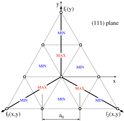
Figure C.1: Orientation of the directions along which the three mapping functions, $f_{1}(y)$, $f_{2}(x,y)$, $f_{3}(x,y)$, are defined. The circles correspond to the positions of atoms, MIN are potential minima, and MAX potential maxima.

The coordinate system $(x,y)$ defined above will be centered at an atomic position; the three directions along which we define the mapping functions $f_{1}(y)$, $f_{2}(x,y)$, $f_{3}(x,y)$ are shown in Fig. C.1. For simplicity, we describe the basis functions by sinusoidal waves with periods $a_{0}\sqrt{3}$, where $a_{0}=a\sqrt{2/3}$ is the period of the lattice along the $x$-axis, and $a$ is the $\langle{100}\rangle$ lattice parameter. The function $f_{1}(y)$ is then written as

$$f_{1}(y)=\sin\left(\frac{2\pi}{a_{0}\sqrt{3}}y\right)\ .$$ (C.1)

Owing to the lattice symmetry which requires the three basis functions to be identical, the functional form of $f_{2}(x,y)$ and $f_{3}(x,y)$ can now be written in a straightforward manner. If we denote $r$ the direction along which $f_{2}$ is defined, the above symmetry requirement and Eq. C.1 demand that $f_{2}(r)=\sin\left(2\pi r/a_{0}\sqrt{3}\right)$. From Fig. C.1, the direction $r$ can be written in terms of $x$ and $y$ as $r=x\cos 30^{\circ}-y\sin 30^{\circ}=x\sqrt{3}/2-y/2$. The basis function $f_{2}$ is then

$$f_{2}(x,y)=\sin\frac{\pi}{a_{0}}\left(x-\frac{y}{\sqrt{3}}\right)\ .$$ (C.2)

The last function, $f_{3}$, can be found in a similar fashion as $f_{2}$. The direction $r$ along which $f_{3}$ is applied is $r=-x\sqrt{3}/2-y/2$. After substituting $r$ in $f_{3}(r)=\sin\left(2\pi r/a_{0}\sqrt{3}\right)$, the last basis function can be written as

$$f_{3}(x,y)=\sin\frac{\pi}{a_{0}}\left(-x-\frac{y}{\sqrt{3}}\right)\ .$$ (C.3)

The mapping function can now be defined as a product of the three basis functions $f_{1}f_{2}f_{3}$ that varies between $\pm 3\sqrt{3}/8$. For practical calculations, we further require that the minimum of $m$ is zero and its height one, which can be easily accomplished by scaling and shifting the product $f_{1}f_{2}f_{3}$. The obtained mapping function then reads:

$$m(x,y)=\frac{1}{2}+\frac{4}{3\sqrt{3}}\sin{\left(\frac{2\pi}{a_{0}\sqrt{3}}y\right)}\,\sin{\frac{\pi}{a_{0}}\left(\frac{y}{\sqrt{3}}-x\right)}\,\sin{\frac{\pi}{a_{0}}\left(\frac{y}{\sqrt{3}}+x\right)}\ .$$ (C.4)

In the final step, we will displace the origin of $m$ into one of the potential minima designated in Fig. C.1 as MIN. One possibility is to change the variables in Eq. C.4 by substituting $x\rightarrow x+a_{0}/2$, $y\rightarrow y+a_{0}\sqrt{3}/6$, which then yields

$$m(x,y)=\frac{1}{2}+\frac{4}{3\sqrt{3}}\sin{\frac{\pi}{3a_{0}}\left(2y\sqrt{3}+a_{0}\right)}\,\sin{\frac{\pi}{a_{0}}\left(\frac{y}{\sqrt{3}}-x-\frac{a_{0}}{3}\right)}\,\sin{\frac{\pi}{a_{0}}\left(\frac{y}{\sqrt{3}}+x+\frac{2a_{0}}{3}\right)}\ .$$ (C.5)

This is the final form of the mapping function, shown in Fig. C.2, that is used in our construction of the Peierls potentials for molybdenum and tungsten. In this Thesis, the contour plots of the mapping function and the Peierls potential are always depicted with the $y$-axis pointing downwards. For this particular choice of sinusoidal basis functions, we arrived at the mapping function that is identical to the unstressed Peierls potential of Edagawa et al., (1997).

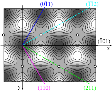
Figure C.2: Contour plot of the mapping function (C.5) of the Peierls potential.

Appendix D Fitted parameters of $\boldsymbol{\tau^{*}_{cr}(T,\dot{\gamma})}$

In this appendix, we list the values of the adjustable constants entering the functions $a,a^{\prime},b,b^{\prime}$ that are involved in the approximations of the stress dependence of the activation enthalpy in Section 6.1 (restricted model) and in Section 6.2 (full model). The restricted model is valid only for loading by pure shear stress parallel to the slip direction, $\sigma$, acting in the MRSSP defined by the angle $\chi$. The full model adds also the effect of the shear stress perpendicular to the slip direction, $\tau$, quantified by the ratio $\eta=\tau/\sigma$. The angles $\chi$ are in radians.

D.1 Parameters for bcc molybdenum

D.1.1 Restricted model

For $\sigma/C_{44}\leq 0.003$:

$a(\chi)=a_{0}+a_{1}\chi+a_{2}\chi^{2}$
$a_{0}$	$a_{1}$	$a_{2}$
71.0798	-12.3631	-30.9276

$b(\chi)=b_{0}+b_{1}\chi+b_{2}\chi^{2}$
$b_{0}$	$b_{1}$	$b_{2}$
0.8331	-0.0163	-0.0052

For $\sigma/C_{44}\geq 0.003$:

$a^{\prime}(\chi)=a^{\prime}_{0}+a^{\prime}_{1}\chi+a^{\prime}_{2}\chi^{2}$
$a^{\prime}_{0}$	$a^{\prime}_{1}$	$a^{\prime}_{2}$
1.3632	-0.0642	-0.0078

$b^{\prime}(\chi)=b^{\prime}_{0}+b^{\prime}_{1}\chi+b^{\prime}_{2}\chi^{2}$
$b^{\prime}_{0}$	$b^{\prime}_{1}$	$b^{\prime}_{2}$
0.0026	0.0002	0.0014

D.1.2 Full model

For $\sigma/C_{44}\leq 0.003$:

$$a(\chi,\eta)=a_{0}(\eta)+a_{1}(\eta)\chi+a_{2}(\eta)\chi^{2}$$

$$\left[\begin{array}[]{c}a_{0}(\eta)\\ a_{1}(\eta)\\ a_{2}(\eta)\end{array}\right]=\left[\begin{array}[]{rrr}71.0798&17.1061&1.6924\\ -12.3631&-19.7773&-2.8968\\ -30.9276&-32.1963&-1.7529\\ \end{array}\right]\left[\begin{array}[]{c}1\\ \eta\\ \eta^{2}\end{array}\right]$$ (D.10)

$$b(\chi,\eta)=b_{0}(\eta)+b_{1}(\eta)\chi+b_{2}(\eta)\chi^{2}$$

$$\left[\begin{array}[]{c}b_{0}(\eta)\\ b_{1}(\eta)\\ b_{2}(\eta)\end{array}\right]=\left[\begin{array}[]{rrr}0.8331&0.0236&-0.0005\\ -0.0163&-0.0254&0.0010\\ -0.0052&-0.0415&0.0049\\ \end{array}\right]\left[\begin{array}[]{c}1\\ \eta\\ \eta^{2}\end{array}\right]$$ (D.20)

For $\sigma/C_{44}\geq 0.003$:

$$a^{\prime}(\chi,\eta)=a^{\prime}_{0}(\eta)+a^{\prime}_{1}(\eta)\chi+a^{\prime}_{2}(\eta)\chi^{2}$$

$$\left[\begin{array}[]{c}a^{\prime}_{0}(\eta)\\ a^{\prime}_{1}(\eta)\\ a^{\prime}_{2}(\eta)\end{array}\right]=\left[\begin{array}[]{rrr}1.3632&0.0962&-0.0099\\ -0.0642&-0.1121&0.0071\\ -0.0078&-0.1020&0.0892\\ \end{array}\right]\left[\begin{array}[]{c}1\\ \eta\\ \eta^{2}\end{array}\right]$$ (D.30)

$$b^{\prime}(\chi,\eta)=b^{\prime}_{0}(\eta)+b^{\prime}_{1}(\eta)\chi+b^{\prime}_{2}(\eta)\chi^{2}$$

$$\left[\begin{array}[]{c}b^{\prime}_{0}(\eta)\\ b^{\prime}_{1}(\eta)\\ b^{\prime}_{2}(\eta)\end{array}\right]=\left[\begin{array}[]{rrr}0.0026&-0.0001&0\\ 0.0002&0.0001&0\\ 0.0014&0.0003&0.0002\\ \end{array}\right]\left[\begin{array}[]{c}1\\ \eta\\ \eta^{2}\end{array}\right]$$ (D.40)

D.2 Parameters for bcc tungsten

D.2.1 Restricted model

For $\sigma/C_{44}\leq 0.003$:

$a(\chi)=a_{0}+a_{1}\chi+a_{2}\chi^{2}$
$a_{0}$	$a_{1}$	$a_{2}$
82.6712	0	-35.4748

$b(\chi)=b_{0}+b_{1}\chi+b_{2}\chi^{2}$
$b_{0}$	$b_{1}$	$b_{2}$
0.8441	0	-0.0013

For $\sigma/C_{44}\geq 0.003$:

$a^{\prime}(\chi)=a^{\prime}_{0}+a^{\prime}_{1}\chi+a^{\prime}_{2}\chi^{2}$
$a^{\prime}_{0}$	$a^{\prime}_{1}$	$a^{\prime}_{2}$
1.3500	0	0.0257

$b^{\prime}(\chi)=b^{\prime}_{0}+b^{\prime}_{1}\chi+b^{\prime}_{2}\chi^{2}$
$b^{\prime}_{0}$	$b^{\prime}_{1}$	$b^{\prime}_{2}$
0.0023	0	0.0013

D.2.2 Full model

For $\sigma/C_{44}\leq 0.003$:

$$a(\chi,\eta)=a_{0}(\eta)+a_{1}(\eta)\chi+a_{2}(\eta)\chi^{2}$$

$$\left[\begin{array}[]{c}a_{0}(\eta)\\ a_{1}(\eta)\\ a_{2}(\eta)\end{array}\right]=\left[\begin{array}[]{rrr}82.6712&51.8676&14.0694\\ 0&26.6283&11.8285\\ -35.4748&-108.8250&-38.7510\\ \end{array}\right]\left[\begin{array}[]{c}1\\ \eta\\ \eta^{2}\end{array}\right]$$ (D.50)

$$b(\chi,\eta)=b_{0}(\eta)+b_{1}(\eta)\chi+b_{2}(\eta)\chi^{2}$$

$$\left[\begin{array}[]{c}b_{0}(\eta)\\ b_{1}(\eta)\\ b_{2}(\eta)\end{array}\right]=\left[\begin{array}[]{rrr}0.8441&0.0616&-0.0018\\ 0&0.0326&-0.0003\\ -0.0013&-0.1118&0.0116\\ \end{array}\right]\left[\begin{array}[]{c}1\\ \eta\\ \eta^{2}\end{array}\right]$$ (D.60)

For $\sigma/C_{44}\geq 0.003$:

$$a^{\prime}(\chi,\eta)=a^{\prime}_{0}(\eta)+a^{\prime}_{1}(\eta)\chi+a^{\prime}_{2}(\eta)\chi^{2}$$

$$\left[\begin{array}[]{c}a^{\prime}_{0}(\eta)\\ a^{\prime}_{1}(\eta)\\ a^{\prime}_{2}(\eta)\end{array}\right]=\left[\begin{array}[]{rrr}1.3500&0.2027&-0.0496\\ 0&0.1160&-0.0454\\ 0.0257&-0.2456&0.1395\\ \end{array}\right]\left[\begin{array}[]{c}1\\ \eta\\ \eta^{2}\end{array}\right]$$ (D.70)

$$b^{\prime}(\chi,\eta)=b^{\prime}_{0}(\eta)+b^{\prime}_{1}(\eta)\chi+b^{\prime}_{2}(\eta)\chi^{2}$$

$$\left[\begin{array}[]{c}b^{\prime}_{0}(\eta)\\ b^{\prime}_{1}(\eta)\\ b^{\prime}_{2}(\eta)\end{array}\right]=\left[\begin{array}[]{rrr}0.0023&-0.0004&0\\ 0&-0.0002&0\\ 0.0013&0.0006&0\\ \end{array}\right]\left[\begin{array}[]{c}1\\ \eta\\ \eta^{2}\end{array}\right]$$ (D.80)

References

- Ackermann et al., (1983) Ackermann, F., Mughrabi, H., and Seeger, A. (1983). Temperature and strain-rate dependence of the flow stress of ultrapure niobium single crystals in cyclic deformation. Acta Metall., 31(9):1353–1366.
- Allen and Tildesley, (1987) Allen, M. P. and Tildesley, D. J. (1987). Computer simulation of liquids. Oxford University Press.
- Allen et al., (1956) Allen, N. P., Hopkins, B. E., and McLennan, J. E. (1956). The tensile properties of single crystals of high-purity iron at temperatures from 100 to -253 C. Proc. R. Soc. Lond. A, 234:221–246.
- Andersen et al., (1985) Andersen, O. K., Jepsen, O., and Glötzel, D. (1985). Canonical description of the band structure of metals. In Bassani, F., Fumi, F., and Tosi, M. P., editors, Highlights of Condensed Matter Theory, page 59. North Holland, Amsterdam.
- Andersen et al., (1994) Andersen, O. K., Jepsen, O., and Krieg, G. (1994). In Kumar, V., Anderson, O. K., and Mookerjee, A., editors, Lectures on Methods of Electronic Structure Calculations, page 63. World Scientific, Singapore.
- Aoki et al., (2007) Aoki, M., Nguyen-Manh, D., Pettifor, D. G., and Vitek, V. (2007). Atom-based bond-order potentials for modelling mechanical properties of metals. Progress of Mat. Sci., 52:154–195.
- Aono et al., (1989) Aono, Y., Kuramoto, E., Brunner, D., and Diehl, J. (1989). Plastic behavior of high-purity molybdenum single crystals in tension and compression. In Strength of metals and alloys (ICSMA8): Proceedings of the 8th international conference, pages 271–276. Pergamon Press.
- Aono et al., (1981) Aono, Y., Kuramoto, E., and Kitajima, K. (1981). Plastic deformation of high-purity iron single crystals. Reports of Res. Inst. for Appl. Mech., 29(92):127–189.
- Aono et al., (1983) Aono, Y., Kuramoto, E., and Kitajima, K. (1983). Fundamental plastic behaviors in high-purity BCC metals (Nb, Mo and Fe). In Strength of metals and alloys (ICSMA6): proceedings of the 6th international conference, pages 9–14. Pergamon Press.
- Argon and Maloof, (1966) Argon, A. S. and Maloof, S. R. (1966). Plastic deformation of tungsten single crystals at low temperatures. Acta Metall., 14:1449–1462.
- Arsenault, (1964) Arsenault, R. J. (1964). Low-temperature creep of alpha iron. Acta Metall., 12:547–554.
- Basinski et al., (1981) Basinski, Z. S., Duesbery, M. S., and Murty, G. S. (1981). The orientation and temperature dependence of plastic flow in potassium. Acta Metall., 29(5):801–807.
- Basinski et al., (1971) Basinski, Z. S., Duesbery, M. S., and Taylor, R. (1971). Influence of shear stress on screw dislocations in a model sodium lattice. Can. J. Phys., 49(16):2160.
- Baskes, (1992) Baskes, M. (1992). Modified embedded-atom potentials for cubic materials and impurities. Phys. Rev. B, 46:2727–2742.
- Bassani, (1994) Bassani, J. L. (1994). Plastic flow of crystals. In Advances in applied mechanics, volume 30, pages 191–258. Academic Press.
- Bolton and Taylor, (1972) Bolton, C. J. and Taylor, G. (1972). Anomalous slip in high-purity niobium single crystals deformed at 77 K in tension. Phil. Mag., 26(6):1359–1376.
- Bowen and Taylor, (1977) Bowen, D. K. and Taylor, G. (1977). The deformation behaviour of dilute niobium-nitrogen alloys. Acta Metall., 25:417–436.
- Brunner, (2004) Brunner, D. (2004). Peculiarities of work hardening of high-purity tungsten single crystals below 800 K. Mat. Sci. Eng. A, 387-389:167–170.
- Brunner and Glebovsky, (2000) Brunner, D. and Glebovsky, V. (2000). Analysis of flow-stress measurements of high-purity tungsten single crystals. Mater. Lett., 44:144–152.
- Bulatov et al., (1998) Bulatov, V. V., Abraham, F. F., Kubin, L., Devincre, B., and Yip, S. (1998). Connecting atomistic and mesoscale simulations of crystal plasticity. Nature, 391:669–671.
- Bulatov and Cai, (2002) Bulatov, V. V. and Cai, W. (2002). Nodal effects in dislocation mobility. Phys. Rev. Lett., 89(11):115501.
- Caillard and Martin, (2003) Caillard, D. and Martin, J. L. (2003). Thermally activated mechanisms in crystal plasticity. Pergamon Press.
- (23) Carlsson, A. E. (1990a). Beyond pair potentials in elemental transition metals and semiconductors. In Ehrenreich, H. and Turnbull, D., editors, Solid State Physics, volume 43, page 1. Academic Press, New York.
- (24) Carlsson, A. E. (1990b). Derivation of angular forces for semiconductors and transition metals. In Nieminen, R. M., Puska, M. J., and Manninen, M. J., editors, Many-Atom Interactions in Solids, page 257. Springer, Heidelberg.
- Cawkwell, (2005) Cawkwell, M. J. (2005). Interatomic bonding and plastic deformation in iridium and molybdenum disilicide. PhD thesis, University of Pennsylvania.
- Cawkwell et al., (2006) Cawkwell, M. J., Nguyen-Manh, D., Pettifor, D. J., and Vitek, V. (2006). Construction, assessment, and application of a bond-order potential for iridium. Phys. Rev. B, 73:064104.
- Celli et al., (1963) Celli, V., Kabler, M., Ninomiya, T., and Thomson, R. (1963). Theory of dislocation mobility in semiconductors. Phys. Rev., 131(1):58–72.
- Chaussidon et al., (2006) Chaussidon, J., Fivel, M., and Rodney, D. (2006). The glide of screw dislocations in bcc Fe: Atomistic static and dynamic simulations. Acta Mater., 54:3407–3416.
- Christian, (1983) Christian, J. W. (1983). Some surprising features of the plastic deformation of body-centered cubic metals and alloys. Metall. Trans. A, 14:1237–1256.
- Conrad and Hayes, (1963) Conrad, H. and Hayes, W. (1963). Thermally-activated deformation of the bcc metals at low temperatures. Trans. ASM, 56:249–262.
- Creten et al., (1977) Creten, R., Bressers, J., and De Meester, P. (1977). Anomalous slip in high-purity vanadium crystals deformed in compression. Mat. Sci. Eng., 29(1):51–53.
- Dagens et al., (1975) Dagens, L., Rasolt, M., and Taylor, R. (1975). Change densities and interionic potentials in simple metals: Nonlinear effects. II. Phys. Rev. B, 11(8):2726–2734.
- Dorn and Rajnak, (1964) Dorn, J. E. and Rajnak, S. (1964). Nucleation of kink pairs and the Peierls’ mechanism of plastic deformation. Trans. AIME, 230:1052–1064.
- Drautz et al., (2005) Drautz, R., Murdick, D. A., Nguyen-Manh, D., Zhou, X. W., Wadley, H. N. G., and Pettifor, D. G. (2005). Analytic bond-order potential for predicting structural trends across the sp-valent elements. Phys. Rev. B, 72(14):144105.
- Duesbery and Richardson, (1991) Duesbery, M. D. and Richardson, G. Y. (1991). The dislocation core in crystalline materials. CRC Critical Reviews in Solid State and Materials Science, 17:1.
- Duesbery, (1969) Duesbery, M. S. (1969). The influence of core structure on dislocation mobility. Phil. Mag., 19(159):501–526.
- Duesbery, (1984) Duesbery, M. S. (1984). On non-glide stresses and their influence on the screw dislocation core in body-centered cubic metals. 1. The Peierls stress. Proc. R. Soc. Lond. A, 392(1802):145–173.
- Duesbery, (1989) Duesbery, M. S. (1989). The dislocation core and plasticity. In Nabarro, F. R. N., editor, Dislocations in Solids, volume 8, pages 66–173. Elsevier.
- Duesbery and Basinski, (1993) Duesbery, M. S. and Basinski, Z. S. (1993). The flow stress of potassium. Acta Metall. Mater., 41(2):643–647.
- Duesbery and Foxall, (1969) Duesbery, M. S. and Foxall, R. A. (1969). A detailed study of deformation of high-purity niobium single crystals. Phil. Mag., 20(166):719.
- Duesbery and Vitek, (1998) Duesbery, M. S. and Vitek, V. (1998). Plastic anisotropy in bcc transition metals. Acta Mater., 46(5):1481–1492.
- Duesbery et al., (2002) Duesbery, M. S., Vitek, V., and Cserti, J. (2002). Non-Schmid plastic behaviour in BCC metals and alloys. In Humphreys, C. J., editor, Understanding materials: A Festschrift for Sir Peter Hirch, pages 165–192. Maney Publishing, Leeds.
- Edagawa et al., (1997) Edagawa, K., Suzuki, T., and Takeuchi, S. (1997). Motion of a screw dislocation in a two-dimensional Peierls potential. Phys. Rev. B, 55(10):6180–6187.
- Elam, (1926) Elam, C. F. (1926). Tensile tests of large gold, silver and copper crystals. Proc. Roy. Soc. A, 112(760):289–296.
- Eshelby and Stroh, (1951) Eshelby, J. D. and Stroh, A. N. (1951). Dislocations in thin plates. Philos. Mag., 42(335):1401–1405.
- Frederiksen and Jacobsen, (2003) Frederiksen, S. L. and Jacobsen, K. W. (2003). Density functional theory studies of screw dislocation core structures in bcc metals. Phil. Mag., 83(3):365–375.
- Friedel, (1969) Friedel, J. (1969). The Physics of Metals, page 340. Cambridge University Press.
- Garrat-Reed and Taylor, (1979) Garrat-Reed, A. J. and Taylor, G. (1979). Optical and electron microscopy of niobium crystals deformed below room temperature. Phil. Mag. A, 39(5):597–646.
- Girshick, (1997) Girshick, A. (1997). Atomistic studies of dislocations in titanium and titanium-aluminum compound. PhD thesis, University of Pennsylvania.
- Girshick et al., (1998) Girshick, A., Bratkovsky, A. M., Pettifor, D. G., and Vitek, V. (1998). Atomistic simulation of titanium - I. A bond-order potential. Phil. Mag. A, 77(4):981–997.
- Goodwin et al., (1989) Goodwin, L., Skinner, A. J., and Pettifor, D. G. (1989). Generating transferable tight-binding parameters - application to silicon. Europhys. Lett., 9(7):701–706.
- Gröger and Vitek, (2005) Gröger, R. and Vitek, V. (2005). Breakdown of the Schmid law in bcc molybdenum related to the effect of shear stress perpendicular to the slip direction. Mat. Sci. Forum, 482:123–126.
- Guiu, (1969) Guiu, F. (1969). Slip asymmetry in molybdenum single crystals deformed in direct shear. Scr. Metall., 3:449–454.
- (54) Henkelman, G., Jóhannesson, G., and Jónsson, H. (2000a). Methods for finding saddle points and minimum energy paths. In Schwartz, S. D., editor, Progress on theoretical chemistry and physics, pages 269–300. Kluwer.
- Henkelman and Jónsson, (2000) Henkelman, G. and Jónsson, H. (2000). Improved tangent estimate in the nudged elastic band method for finding minimum energy paths and saddle points. J. Chem. Phys., 113(22):9978–9985.
- (56) Henkelman, G., Uberuaga, B. P., and Jónsson, H. (2000b). A climbing image nudged elastic band method for finding saddle points and minimum energy paths. J. Chem. Phys., 113(22):9901–9904.
- Hill and Rice, (1972) Hill, J. R. and Rice, R. (1972). Constitutive analysis of elastic-plastic crystals at arbitrary strain. J. Mech. Phys. Sol., 20:401–413.
- Hill, (1965) Hill, R. (1965). Continuum micro-mechanics of elastoplastic polycrystals. J. Mech. Phys. Sol., 13:89–101.
- Hill and Havner, (1982) Hill, R. and Havner, K. S. (1982). Perspectives in the mechanics of elastoplastic crystals. J. Mech. Phys. Sol., 30:5–22.
- Hirsch, (1960) Hirsch, P. B. (1960). In 5th Int. Conf. on Crystallography, Cambridge.
- Hirsch, (1980) Hirsch, P. B. (1980). Direct observations of dislocations by transmission electron microscopy: recollections of the period 1946-56. Proc. R. Soc. Lond. A, 371:160–164.
- Hirsch et al., (1956) Hirsch, P. B., Horne, R. W., and Whelan, M. J. (1956). Direct observations of the arrangement and motion of dislocations in aluminum. Phil. Mag., 1:677.
- Hirth and Lothe, (1982) Hirth, J. P. and Lothe, J. (1982). Theory of dislocations. J.Wiley & Sons, 2 edition.
- Hirth and Nix, (1969) Hirth, J. P. and Nix, W. D. (1969). An analysis of the thermodynamics of dislocation glide. Phys. Stat. Sol., 35:177–187.
- Hollang, (2001) Hollang, L. (2001). Mechanical properties. In Waseda, Y. and Isshiki, M., editors, Purification process and characterization of ultra high purity metals. Springer-Verlag.
- Hollang et al., (2001) Hollang, L., Brunner, D., and Seeger, A. (2001). Work hardening and flow stress of ultrapure molybdenum single crystals. Mat. Sci. Eng. A, 319-321:233–236.
- Hollang et al., (1997) Hollang, L., Hommel, M., and Seeger, A. (1997). The flow stress of ultra-high-purity molybdenum single crystals. Phys. Stat. Sol. (a), 160(2):329–354.
- Horsfield et al., (1996) Horsfield, A. P., Bratkovsky, A. M., Fearn, M., Pettifor, D. G., and Aoki, M. (1996). Bond-Order potentials: Theory and implementation. Phys. Rev. B, 53(19):12694–12712.
- Hull and Bacon, (2001) Hull, D. and Bacon, D. J. (2001). Introduction to dislocations. Butterworth-Heinemann, Oxford, 4th edition.
- Ismail-Beigi and Arias, (2000) Ismail-Beigi, S. and Arias, T. A. (2000). Ab initio study of screw dislocations in Mo and Ta: A new picture of plasticity in bcc transition metals. Phys. Rev. Lett., 84(7):1499–1502.
- Ito and Vitek, (2001) Ito, K. and Vitek, V. (2001). Atomistic study of non-Schmid effects in the plastic yielding of bcc metals. Phil. Mag. A, 81(5):1387–1407.
- Jeffcoat et al., (1976) Jeffcoat, P. J., Mordike, B. L., and Rogausch, K. D. (1976). Anomalous slip in Mo-5 at.% Nb and Mo-5 at.% Re alloy single crystals. Phil. Mag., 34(4):583–592.
- Jeffrey, (2000) Jeffrey, A. (2000). Handbook of mathematical formulas and integrals. Academic Press, 2nd edition.
- Jonsson, (2003) Jonsson, A. (2003). Discrete dislocation dynamics by an O(N) algorithm. Comp. Mat. Sci., 27:271–288.
- Jónsson et al., (1998) Jónsson, H., Mills, G., and Jacobsen, K. W. (1998). Nudged elastic band method for finding minimum energy paths of transitions. Classical and Quantum Dynamics in Condensed Phase Simulations. World Scientific.
- Kaspar et al., (2000) Kaspar, J., Luft, A., and Skrotzki, W. (2000). Deformation modes and structure evolution in laser-shock-loaded molybdenum single crystals of high purity. Cryst. Res. Technol., 35(4):437–448.
- Kaun et al., (1968) Kaun, L., Luft, A., Richter, J., and Schulze, D. (1968). Slip line pattern and active slip systems of tungsten and molybdenum single crystals weakly deformed in tension at room temperature. Phys. Stat. Sol., 26(2):485.
- Keh, (1965) Keh, A. S. (1965). Work hardening and deformation sub-structure in iron single crystals deformed in tension at 298 K. Phil. Mag., 12:9–30.
- Kitajima et al., (1981) Kitajima, K., Aono, Y., and Kuramoto, E. (1981). Slip systems and orientation dependence of yield stress in high purity molybdenum single crystals at 4.2 K and 77 K. Scripta Metall., 15:919–924.
- Kocks et al., (1975) Kocks, U. F., Argon, A. S., and Ashby, M. F. (1975). Thermodynamics and kinetics of slip. Progress in Materials Science, 19:1–291.
- Kubin et al., (1998) Kubin, L., Devincre, B., and Tang, M. (1998). Mesoscopic modelling and simulation of plasticity in fcc and bcc crystals: Dislocation intersections and mobility. J. Comp.-Aid. Mat. Design, 5:31–54.
- Lassila et al., (2002) Lassila, D. H., LeBlanc, M. M., and Kay, G. J. (2002). Uniaxial stress deformation experiment for validation of 3-D dislocation dynamics simulations. J. Eng. Mat. Tech., 124:290–296.
- Lassila et al., (2003) Lassila, D. H., LeBlanc, M. M., and Rhee, M. (2003). Single crystal deformation experiments for validation of dislocation dynamics simulations. In MRS Symp. Proc., volume 779, pages W2.9.1–2.9.12.
- Lau and Dorn, (1970) Lau, S. S. and Dorn, J. E. (1970). Asymmetric slip in Mo single crystals. Phys. Stat. Sol. A, 2:825–836.
- Liu et al., (2005) Liu, G., Nguyen-Manh, D., Liu, B.-G., and Pettifor, D. G. (2005). Magnetic properties of point defects in iron within the tight-binding-bond Stoner model. Phys. Rev. B, 71:174115.
- Louchet, (2003) Louchet, F. (2003). http://www.gpm2.inpg.fr/axes/plast/MicroPlast/ddd/TEM.
- Louchet and Kubin, (1975) Louchet, F. and Kubin, L. P. (1975). Dislocation substructures in the anomalous slip plane of single crystal niobium strained at 50 K. Acta Metall., 23:17–21.
- Louchet and Kubin, (1979) Louchet, F. and Kubin, L. P. (1979). Dislocation processes in bcc metals. Phys. Stat. Sol. A, 56:169.
- Louchet et al., (1979) Louchet, F., Kubin, L. P., and Vesely, D. (1979). In situ deformation of b.c.c. crystals at low temperatures in a high-voltage electron microscope. Dislocation mechanisms and strain-rate equation. Phil. Mag. A, 39(4):433–454.
- Maragakis et al., (2002) Maragakis, P., Andreev, S. A., Brumer, Y., Reichman, D. R., and Kaxiras, E. (2002). Adaptive nudged elastic band approach for transition state calculation. J. Chem. Phys., 117(10):4651–4658.
- Marian et al., (2004) Marian, J., W., C., and Bulatov, V. V. (2004). Dynamic transitions from smooth to rough to twinning in dislocation motion. Nature Mat., 3:2004.
- Matsui and Kimura, (1976) Matsui, H. and Kimura, H. (1976). Anomalous slip in high-purity molybdenum single crystals and its comparison with that in V(a) metals. Mat. Sci. Eng., 24:247–256.
- Matsui et al., (1982) Matsui, H., Kimura, H., Saka, H., Noda, K., and Imura, T. (1982). Anomalous slip induced by the surface effect in molybdenum single-crystal foils deformed in a high voltage electron microscope. Mat. Sci. Eng., 53:263–272.
- Matterstock et al., (1999) Matterstock, B., Martin, J. L., Bonneville, J., and Kruml, T. (1999). Direct measurement of dislocation exhaustion rates during plastic deformation of ni3al compounds. Mat. Res. Soc. Symp. Proc., 552:KK5.17.1–6.
- McKee and Page, (1993) McKee, M. L. and Page, M. (1993). Computing reaction pathways on molecular potential energy surfaces. In Lipkowitz, K. B. and Boyd, D. B., editors, Reviews in Computational Chemistry, volume 4. VCH Publishers.
- Mendis et al., (2006) Mendis, B. G., Mishin, Y., Hartley, C. S., and Hemker, K. J. (2006). Use of the nye tensor in analyzing hrem images of bcc screw dislocations. Phil. Mag., 86(29-31):4607–4640.
- Meyers et al., (2002) Meyers, M. A., Benson, D. J., Vöhringer, O., Kad, B. K., Xue, Q., and Fu, H.-H. (2002). Constitutive description of dynamic deformation: physically-based mechanisms. Mat. Sci. Eng. A, 322:194–216.
- Mitchell et al., (1963) Mitchell, T. E., Foxall, R. A., and Hirsch, P. B. (1963). Work-hardening in niobium single crystals. Phil. Mag., 8:1895–1920.
- Moriarty, (1988) Moriarty, J. A. (1988). Density-functional formulation of the generalized pseudopotential theory: III. Transition-metal interatomic potentials. Phys. Rev. B, 38(5):3199–3231.
- Moriarty, (1990) Moriarty, J. A. (1990). Analytic representation of multi-ion interatomic potentials in transition metals. Phys. Rev. B, 42(3):1609–1628.
- Moriarty et al., (2002) Moriarty, J. A., Vitek, V., Bulatov, V. V., and Yip, S. (2002). Atomistic simulations of dislocations and defects. J. Comp.-Aid. Mat. Design, 9:99.
- Mrovec, (2002) Mrovec, M. (2002). Bond order potentials for bcc transition metals and molybdenum silicides. PhD thesis, University of Pennsylvania.
- Mrovec et al., (2007) Mrovec, M., Gröger, R., Bailey, A. G., Nguyen-Manh, D., Elsässer, C., and Vitek, V. (2007). Bond-order potential for simulations of extended defects in tungsten. Phys. Rev. B, 75:104119.
- Mrovec et al., (2004) Mrovec, M., Nguyen-Manh, D., Pettifor, D. G., and Vitek, V. (2004). Bond-order potential for molybdenum: Application to dislocation behavior. Phys. Rev. B, 69:094115.
- Murdick et al., (2006) Murdick, D. A., Zhou, X. W., Wadley, H. N. G., Nguyen-Manh, D., Drautz, R., and Pettifor, D. G. (2006). Analytic bond-order potential for the gallium arsenide system. Phys. Rev. B, 73(4):045206.
- Nabarro, (1947) Nabarro, F. R. N. (1947). Dislocations in a simple cubic lattice. Proc. Phys. Soc., 59(2):256–272.
- Nawaz and Mordike, (1975) Nawaz, M. H. A. and Mordike, B. L. (1975). Slip geometry of tantalum and tantalum alloys. Phys. Stat. Sol. A, 32:449–458.
- Nguyen-Manh et al., (2000) Nguyen-Manh, D., Pettifor, D. G., and Vitek, V. (2000). Analytic environment-dependent tight-binding bond integrals: Application to MoSi2. Phys. Rev. Lett., 85(19):4136–4139.
- Orowan, (1934) Orowan, E. (1934). Z. Phys., 89:634.
- Peach and Koehler, (1950) Peach, M. and Koehler, J. S. (1950). The forces exerted on dislocations and the stress fields produced by them. Phys. Rev., 80(3):436–439.
- Peierls, (1940) Peierls, R. (1940). The size of a dislocation. Proc. Phys. Soc., 52(1):34–37.
- Pettifor, (1995) Pettifor, D. G. (1995). Bonding and structure of molecules and solids. Oxford University Press.
- Pettifor et al., (2004) Pettifor, D. G., Finnis, M. W., Nguyen-Manh, D., Murdick, D. A., Zhou, X. W., and Wadley, H. N. G. (2004). Analytic bond-order potentials for multicomponent systems. Mat. Sci. Eng. A, 365(1-2):2–13.
- Pettifor and Oleinik, (2002) Pettifor, D. G. and Oleinik, I. I. (2002). Analytic bond-order potential for open and close-packed phases. Phys. Rev. B, 65(17):172103.
- (115) Pichl, W. and Krystian, M. (1997a). The flow stress of high purity alkali metals. Phys. Stat. Sol. A, 160(2):373–383.
- (116) Pichl, W. and Krystian, M. (1997b). The non-uniform temperature dependence of the flow stress of potassium. Phil. Mag. Lett., 75(2):75–82.
- (117) Pichl, W. and Krystian, M. (1997c). The plasticity of potassium. Mat. Sci. Eng., A234-236:426–429.
- Polanyi, (1934) Polanyi, M. (1934). Z. Phys., 89:660.
- (119) Qin, Q. and Bassani, J. L. (1992a). Non-associated plastic flow in single crystals. J. Mech. Phys. Sol., 40(4):835–862.
- (120) Qin, Q. and Bassani, J. L. (1992b). Non-Schmid yield behavior in single crystals. J. Mech. Phys. Sol., 40(4):813–833.
- Reed and Arsenault, (1976) Reed, R. E. and Arsenault, R. J. (1976). Further observations of anomalous slip in niobium single crystals. Scripta Metall., 10:1003–1006.
- Rice, (1971) Rice, J. R. (1971). Inelastic constitutive relations for solids: An internal-variable theory and its application to metal plasticity. J. Mech. Phys. Sol., 19:433–455.
- Saka et al., (1976) Saka, H., Matsui, H., Noda, K., Kimura, H., and Imura, T. (1976). Direct observation of anomalous slip in molybdenum by HVEM. Scripta Metall., 10:59–62.
- Schmid and Boas, (1935) Schmid, E. and Boas, W. (1935). Kristallplastizität. Springer, Berlin.
- Schoeck, (1965) Schoeck, G. (1965). The activation energy of dislocation movement. Phys. Stat. Sol., 8:499–507.
- Seeger, (1956) Seeger, A. (1956). On the theory of the low-temperature internal friction peak observed in metals. Phil. Mag., 1(7):651–662.
- Seeger, (2004) Seeger, A. (2004). Experimental evidence for the transformation of the screw-dislocation cores in body-centred cubic metals. Phys. Stat. Sol. (a), 201(4):21–24.
- Seeger and Hollang, (2000) Seeger, A. and Hollang, L. (2000). The flow-stress asymmetry of ultra-pure molybdenum single crystals. Mater. Trans., JIM, 41(1):141–151.
- Shields et al., (1975) Shields, J. A., Goods, S. H., Gibala, R., and Mitchell, T. E. (1975). Deformation of high purity tantalum single crystals at 4.2 K. Mat. Sci. Eng., 20:71–81.
- Sigle, (1999) Sigle, W. (1999). High-resolution electron microscopy and molecular dynamics study of the a/2[111] screw dislocations in molybdenum. Phil. Mag. A, 79(5):1009–1020.
- Slater and Koster, (1954) Slater, J. C. and Koster, G. F. (1954). Simplified lcao method for the periodic potential problem. Phys. Rev., 94(6):1498–1524.
- Stoner, (1938) Stoner, E. C. (1938). Collective electron ferromagnetism. Proc. Roy. Soc. London A, 165(922):372–414.
- Stoner, (1939) Stoner, E. C. (1939). Collective electron ferromagnetism: II. Energy and specific heat. Proc. Roy. Soc. London A, 169(938):339–371.
- Strogatz, (2003) Strogatz, S. (2003). Sync: An emergenging science of spontaneous order. Hyperion.
- Sutton et al., (1988) Sutton, A. P., Finnis, M. W., Pettifor, D. G., and Ohta, Y. (1988). The tight-binding bond model. J. Phys. C, 21:35–66.
- Suzuki et al., (1995) Suzuki, T., Koizumi, H., and Kirchner, H. O. K. (1995). Plastic flow stress of bcc transition metals and the Peierls potential. Acta Metall. Mater., 43(6):2177–2187.
- Tabata et al., (1976) Tabata, T., Mori, H., and Fujita, H. (1976). In-situ deformation of tungsten single crystals with [100] tensile axis in an ultra-high voltage electron microscope. J. Phys. Soc. Japan, 40(4):1103–1111.
- Takeuchi and Maeda, (1977) Takeuchi, S. and Maeda, K. (1977). Slip in high purity tantalum between 0.7 and 40 K. Acta Metall., 25:1485–1490.
- Taylor et al., (1973) Taylor, G., Bajaj, R., and Carlson, O. N. (1973). Anomalous slip in high-purity vanadium crystals. Phil. Mag., 28(5):1035–1042.
- Taylor and Saka, (1991) Taylor, G. and Saka, M. (1991). Some observations on slip in niobium and Nb-Ti alloy deformed in situ in a HVEM. Phil. Mag. A, 64(6):1345–1354.
- Taylor, (1928) Taylor, G. I. (1928). The deformation of crystals of -brass. Proc. R. Soc. Lond. A, 118(779):1–24.
- Taylor, (1934) Taylor, G. I. (1934). The mechanism of plastic deformation of crystals. Part I. Theoretical. Proc. Roy. Soc. A, 145(855):362–387.
- Taylor and Elam, (1925) Taylor, G. I. and Elam, C. F. (1925). The plastic extension and fracture of aluminium crystals. Proc. Roy. Soc. A, 108:28–51.
- Taylor and Elam, (1926) Taylor, G. I. and Elam, C. F. (1926). The distortion of iron crystals. Proc. Roy. Soc. A, 112(761):337–361.
- Taylor and Farren, (1926) Taylor, G. I. and Farren, W. S. (1926). The distortion of crystals of aluminium under compression - Part I. Proc. Roy. Soc. A, 111:529–551.
- Vesely, (1968) Vesely, D. (1968). The study of deformation of thin foils of Mo under the electron microscope. Phys. Stat. Sol. A, 29:675–683.
- Vesely, (2006) Vesely, D. (2006). private communication.
- Vineyard, (1957) Vineyard, G. H. (1957). Frequency factors and isotope effects in solid state rate processes. J. Phys. Chem. Solids, 3:121–127.
- Vitek, (1968) Vitek, V. (1968). Intrinsic stacking faults in body-centred cubic crystals. Phil. Mag. A, 18(154):773.
- Vitek, (1992) Vitek, V. (1992). Structure of dislocation cores in metallic materials and its impact on their plastic behaviour. Prog. Mater. Sci., 36:1–27.
- Vitek, (2004) Vitek, V. (2004). Core structure of screw dislocations in body-centred cubic metals: relation to symmetry and interatomic bonding. Philos. Mag., 84(3-5):415–428.
- Vitek et al., (2004) Vitek, V., Mrovec, M., Gröger, R., Bassani, J. L., Racherla, V., and Yin, L. (2004). Effects of non-glide stresses on the plastic flow of single and polycrystals of molybdenum. Mat. Sci. Eng. A, 387-389:138–142.
- Vitek et al., (1970) Vitek, V., Perrin, R. C., and Bowen, D. K. (1970). Core structure of 1/2 screw dislocations in bcc crystals. Philos. Mag., 21(173):1049.
- von Neumann, (1885) von Neumann, J. (1885). Vorlesungen über die Theorie der Elasticität. Leipzig.
- Voyiadjis and Abed, (2005) Voyiadjis, G. Z. and Abed, F. H. (2005). Microstructural based models for bcc and fcc metals with temperature and strain rate dependency. Mech. Mater., 37:355–378.
- Wasserbäch and Novák, (1985) Wasserbäch, W. and Novák, V. (1985). Optical investigation of anomalous slip-line patterns in high purity niobium and tantalum single crystals after tensile deformation at 77 K. Mat. Sci. Eng., 73:197–202.
- Webb et al., (1974) Webb, G. L., Gibala, R., and Mitchell, T. E. (1974). Effect of normal stress on yield asymmetry in high purity tantalum crystals. Metall. Trans., 5(7):1581–1584.
- Wen and Ngan, (2000) Wen, M. and Ngan, A. H. W. (2000). Atomistic simulation of kink-pairs of screw dislocations in body-centred cubic iron. Acta Mater., 48:4255–4265.
- Woodward and Rao, (2001) Woodward, C. and Rao, S. I. (2001). Ab-initio simulation of isolated screw dislocations in bcc Mo and Ta. Phil. Mag. A, 81(5):1305–1316.
- Woodward and Rao, (2002) Woodward, C. and Rao, S. I. (2002). Flexible ab initio boundary conditions: Simulating isolated dislocations in bcc Mo and Ta. Phys. Rev. Lett., 88(21):216402.
- Xu and Moriarty, (1996) Xu, W. and Moriarty, J. A. (1996). Atomistic simulation of ideal shear strength, point defects, and screw dislocations in bcc transition metals: Mo as a prototype. Phys. Rev. B, 54(10):6941–6951.
- Xu and Moriarty, (1998) Xu, W. and Moriarty, J. A. (1998). Accurate atomistic simulations of the Peierls barrier and kink-pair formation energy for screw dislocations in bcc Mo. Comp. Mater. Sci., 9:348–356.
- Yang et al., (2001) Yang, L. H., Söderlind, P., and Moriarty, J. A. (2001). Atomistic simulation of pressure-dependent screw dislocation properties in bcc tantalum. Mat. Sci. Eng. A, 309-310:102–107.
- Zbib et al., (2000) Zbib, H. M., de la Rubia, T. D., Rhee, M., and Hirth, J. P. (2000). 3D dislocation dynamics: stress-strain behavior and hardening mechanisms in fcc and bcc metals. J. Nucl. Mat., 276:154–165.
- Zerilli, (2004) Zerilli, F. J. (2004). Dislocation mechanics-based constitutive equations. Metall. and Mater. Trans. A, 35:2547–2555.
- Zhou et al., (1998) Zhou, S. J., Preston, D. L., Lomdahl, P. S., and Beazley, D. M. (1998). Large-scale molecular dynamics simulations of dislocation intersection in copper. Science, 279:1525–1527.
- Zinkle et al., (2002) Zinkle, S. J., Victoria, M., and Abe, K. (2002). Scientific and engineering advances from fusion materials R&D. J. Nuclear Mat., 307-311:31–42.
- Znam, (2001) Znam, S. (2001). Bond-order potentials for atomistic studies of dislocations and other extended defects in TiAl. PhD thesis, University of Pennsylvania.
- Znam et al., (2003) Znam, S., Nguyen-Manh, D., Pettifor, D. G., and Vitek, V. (2003). Atomistic modelling of TiAl - I. Bond-order potentials with environmental dependence. Phil. Mag., 83(4):415–438.