Relativistic multi-reference Fock-space coupled-cluster calculation of the forbidden 6โ€‹s2โ€‹S01โŸถ6โ€‹sโ€‹5โ€‹d3โ€‹D1โŸถ6superscript๐‘ 2superscriptsubscript๐‘†016๐‘ 5superscript๐‘‘3subscript๐ท16s^{2}\,{}^{1}S_{0}\longrightarrow 6s5d\,^{3}D_{1} magnetic-dipole transition in ytterbium

Chiranjib Sur Department of Astronomy, The Ohio State University Columbus, Ohio, 43210, USA csur@astronomy.ohio-state.edu http://www.astronomy.ohio-state.edu/~csur โ€ƒโ€ƒ Rajat K Chaudhuri Indian Institute of Astrophysics,Bangalore 560034, India
(Phys. Rev. A, 76, 012509 (2007))
Abstract

We report the forbidden 6โ€‹s2โ€‹S01โŸถ6โ€‹sโ€‹5โ€‹d3โ€‹D1โŸถ6superscript๐‘ 2superscriptsubscript๐‘†016๐‘ 5superscript๐‘‘3subscript๐ท16s^{2}\,{}^{1}S_{0}\longrightarrow 6s5d\,^{3}D_{1} magnetic-dipole transition amplitude computed using multi-reference Fock-space coupled-cluster theory. Our computed transition matrix element ($1.34\times 10^{-4}\mu_{B}$) is in excellent agreement with the experimental value ($1.33\times 10^{-4}$ $\mu_{B}$). This value in combination with other known quantities will be helpful to determine the parity non-conserving amplitude for the 6โ€‹s2โ€‹S01โŸถ6โ€‹sโ€‹5โ€‹d3โ€‹D1โŸถ6superscript๐‘ 2superscriptsubscript๐‘†016๐‘ 5superscript๐‘‘3subscript๐ท16s^{2}\,{}^{1}S_{0}\longrightarrow 6s5d\,^{3}D_{1} transition in atomic Yb. To our knowledge our calculation is the most accurate to date and can be very important in the search of physics beyond the standard model. We further report the 6โ€‹sโ€‹6โ€‹p3โ€‹P0โŸถ6โ€‹sโ€‹6โ€‹p1โ€‹P1โŸถ6๐‘ 6superscript๐‘3subscript๐‘ƒ06๐‘ 6superscript๐‘1subscript๐‘ƒ16s6p\,^{3}P_{0}\longrightarrow 6s6p\,^{1}P_{1} and 6โ€‹sโ€‹5โ€‹d3โ€‹D1โŸถ6โ€‹sโ€‹6โ€‹p3โ€‹P0โŸถ6๐‘ 5superscript๐‘‘3subscript๐ท16๐‘ 6superscript๐‘3subscript๐‘ƒ06s5d\,^{3}D_{1}\longrightarrow 6s6p\,^{3}P_{0} transition matrix elements which are also in good agreement with the earlier theoretical estimates.

PACS number(s) : 31.15.Ar, 31.15.Dv, 31.25.-v, 32.70.Cs,

I Introduction

The highly forbidden 6โ€‹s2โ€‹S01โŸถ6โ€‹sโ€‹5โ€‹d3โ€‹D1โŸถ6superscript๐‘ 2superscriptsubscript๐‘†016๐‘ 5superscript๐‘‘3subscript๐ท16s^{2}\,{}^{1}S_{0}\longrightarrow 6s5d\,\,^{3}D_{1} magnetic-dipole ($M1$) transition amplitude in ytterbium (Yb), a key quantity for evaluating the feasibility of parity non-conservation (PNC), has recently been measured by Stalnaker et al. Budker using Stark-interference experiment. The electric-dipole ($E1$) matrix element for 6โ€‹s2โ€‹S01โŸถ6โ€‹sโ€‹5โ€‹d3โ€‹D1โŸถ6superscript๐‘ 2superscriptsubscript๐‘†016๐‘ 5superscript๐‘‘3subscript๐ท16s^{2}\,{}^{1}S_{0}\longrightarrow 6s5d\,\,^{3}D_{1} transition in Yb is forbidden because of its sโˆ’d๐‘ ๐‘‘s-d nature. The forbidden $M1$ transition amplitude mentioned above is therefore the key quantity to explore the feasibility of the PNC study for this transition in Yb. Accurate determination of the $M1$ transition amplitude, which is strongly suppressed in nature in the absence of external fields, can be used together with the large PNC- and moderately large Stark- induced $E1$ amplitudes to understand PNC studies in neutral Yb. Strong configuration mixing and spin-orbit interaction in both the upper and the lower states give rise to a non-zero 6โ€‹s2โ€‹S01โŸถ6โ€‹sโ€‹5โ€‹d3โ€‹D1โŸถ6superscript๐‘ 2superscriptsubscript๐‘†016๐‘ 5superscript๐‘‘3subscript๐ท16s^{2}\,{}^{1}S_{0}\longrightarrow 6s5d\,\,^{3}D_{1} transition amplitude Budker ; Hw . Surprisingly, despite its tremendous importance in PNC experiments, only a rough theoretical estimate ($|A(M1)|\leqslant 10^{-4}\mu_{B}$) is available in the literature for this transition. PNC in atoms arises from the neutral weak interactions and are considerably enhanced in heavy atoms. Combining the high precision experiments and theoretical calculations of PNC observables, it is possible to extract the nuclear weak charge PNC-review . Any discrepancy of its value with the one obtained from the standard model (SM) of particle physics could possibly reveal the existence of new physics beyond the SM.

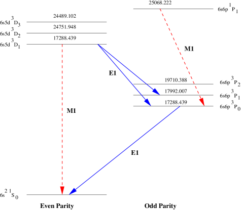
The ground and excited states of closed shell ground state systems like Yb are, in general, multi-configurational in nature, and hence, an accurate description of these states requires a balanced treatment of non-dynamical or configuration mixing and dynamical electron correlation effects (this will be more clear by studying the energy levels in figure 1). It is, therefore, imperative that these systems must be treated with methods which are combinations of the configuration interaction (CI) and many-body perturbation theory (MBPT), such as multi-reference many-body perturbation theories (MR-MBPT) Hv ; MRMP ; PT2 ; Hvr ; Nakano ; Dzuba , multi-reference Fock-space coupled-cluster (MR-FSCC) theories and/or it variants mrcc ; Lindgren ; Mukherjee ; Kaldor ; Pie etc. The state-of-the-art MR-FSCC is an all-order approach and is capable of providing reliable estimates of predicted quantities. In this paper, we employ the MR-FSCC method to compute the magnetic-dipole transition amplitude for 6โ€‹s2โ€‹S01โŸถ6โ€‹sโ€‹5โ€‹d3โ€‹D1โŸถ6superscript๐‘ 2superscriptsubscript๐‘†016๐‘ 5superscript๐‘‘3subscript๐ท16s^{2}\,{}^{1}S_{0}\longrightarrow 6s5d\,\,^{3}D_{1} transition in Yb using four-component relativistic spinors. The resulting value of this magnetic-dipole transition matrix element in atomic Yb is $1.34\times 10^{-4}\mu_{B}$, which differs by less than one percent from the experimental value. In addition, we have also calculated the 6โ€‹sโ€‹6โ€‹p3โ€‹P0โŸถ6โ€‹sโ€‹6โ€‹p1โ€‹P1โŸถ6๐‘ 6superscript๐‘3subscript๐‘ƒ06๐‘ 6superscript๐‘1subscript๐‘ƒ16s6p\,^{3}P_{0}\longrightarrow 6s6p\,^{1}P_{1} $M1$ transition transition amplitude in Yb which plays crucial role in the measurement of the PNC induced electric-dipole amplitude Kimball . This is the first time any variant of coupled-cluster theory has been applied to determine the $M1$ transition amplitude of Yb. A precise determination of this quantity ensures not only the power of the theory but also for the experimental uncertainties. To our knowledge no such theoretical results are available for magnetic dipole transitions in Yb.

The structure of this paper is the following : section I describes the physical relevance of the problem. Section II provides a brief outline of the multi-reference Fock-space CC (MR-FSCC) theory for two-electron attachment processes that is used to compute the M1 transition elements between the ground ${}^{1}S_{0}$ and excited ${}^{3}D_{1}$ state. Section III contains the results of our calculation with an in-depth discussion. Finally in section IV we conclude and highlight the findings of our paper.

Refer to caption
Figure 1: Energy levels of the ground and low lying excited states of Yb. The energies (in $\mathrm{cm}^{-1}$) are given with respect to the ground state and are obtained from the NIST database NIST . Electric dipole (allowed) and magnetic dipole (forbidden) transitions are represented by โ€˜blueโ€™ (solid) and โ€˜redโ€™ (dashed) lines respectively. This diagram helps us to understand the requirement of a multi-reference theory to describe the atomic states of Yb.

II Fock-space multi-reference coupled-cluster (mr-fscc) theory for two-electron attachment processes

In MR-FSCC method Lindgren ; Haque ; Mukherjee ; LindMukh ; Sinha ; Pal ; Kaldor , the self-consistent field (SCF) solution of the Hartree-Fock (Dirac- Fock in relativistic regime) for the $N$-electron closed shell ground state $\Phi_{\mathrm{HF/DF}}$ is chosen as the vacuum (for labeling purpose only) to define holes and particles with respect to $\Phi_{\mathrm{HF/DF}}$. The multi-reference aspect is then introduced by subdividing the hole and particle orbitals into active and inactive categories, where different occupations of the active orbitals will define a multi-reference model space for our problem. We call a model space to be complete if it has all possible electron occupancies in the active orbitals, otherwise incomplete. The classification of orbitals into active and inactive groups is, in principle, arbitrary and is at our disposal. However, for the sake of computational convenience, we treat only a few hole and particle orbitals as active, namely those are close to the Fermi level. The classification of orbitals is depicted schematically in Fig.2(a). Diagrammatically, active holes and particles are depicted as solid lines with double arrows and the corresponding inactive lines are designated by dotted lines with single arrow. The orbitals which can be both active and inactive are designated by solid lines with single arrow (see Fig.2(b)).

We designate by $\Psi_{i}^{0(k,l)}$ a model space of $k$-hole and $l$-particle determinants, where in the present instance ($\mathrm{Yb}^{+2}+2e\longrightarrow\mathrm{Yb}$), $k=0$ and $l$ ranges from 0 to 2. Generally, any second quantized operator has $k$-hole and $l$-particle annihilation operators for the active holes and particles. For convenience, we indicate the โ€œhole-particle valence rankโ€ of an operator by a superscript ($k,l$) on the operator. Thus, according to our notation, an operator $A^{(k,l)}$ will have exactly $k$-hole and $l$-particle annihilation operators.

Refer to caption
Figure 2: (a) Schematic depiction of the classification of particle and hole orbitals into active and inactive categories. (b) Diagrammatic representation of hole ($\downarrow$), particles ($\uparrow$), active particles (double up arrow), inactive holes, and particles (dashed down/up arrow). (c) Diagrammatic representation of $S^{(0,0)}$ $(T)$, $S^{(0,1)}$, and $S^{(0,2)}$ cluster operators.

We now describe the type of ansatz used to derive the MR-FSCC equations for direct energy difference calculations in two-electron attachment processes. The Hartree-Fock/Dirac-Fock function $\Phi_{\mathrm{HF/DF}}$ is denoted by $\Psi^{(0,0)}$ and the inactive hole and particle orbitals (defined with respect to $\Phi_{\mathrm{HF/DF}}$) are labeled by the indices $a,b,c,\cdots$ and $p,q,r,\cdots$, respectively. The corresponding active holes and particles are labeled by the indices $\alpha,\beta,\gamma\cdots$ and $u,v,w\cdots$, respectively. Note that there will be no active holes (particles) for two electron attachment (detachment) processes. The cluster operator correlating the $N$-electron ground/reference state is denoted in our notation by $S^{(0,0)}$ which can be split into various $n$-body components depending upon the various hole-particle excitation ranks. The cluster operator $S^{(0,0)}$ upto 2-body (first two diagrams of Fig.2(c)) can be written in second quantized notation as,

S(0,0)=S1(0,0)+S2(0,0)+โ‹ฏ=โˆ‘p,aโŸจp|s1(0,0)|aโŸฉโ€‹{apโ€ โ€‹aa}+14โ€‹โˆ‘a,b,p,qโŸจpโ€‹q|s2(0,0)|aโ€‹bโŸฉโ€‹{apโ€ โ€‹aqโ€ โ€‹abโ€‹aa}+โ‹ฏsuperscript๐‘†00superscriptsubscript๐‘†100superscriptsubscript๐‘†200โ‹ฏsubscript๐‘๐‘Žquantum-operator-product๐‘superscriptsubscript๐‘ 100๐‘Žsuperscriptsubscript๐‘Ž๐‘โ€ subscript๐‘Ž๐‘Ž14subscript๐‘Ž๐‘๐‘๐‘žquantum-operator-product๐‘๐‘žsuperscriptsubscript๐‘ 200๐‘Ž๐‘superscriptsubscript๐‘Ž๐‘โ€ superscriptsubscript๐‘Ž๐‘žโ€ subscript๐‘Ž๐‘subscript๐‘Ž๐‘Žโ‹ฏS^{(0,0)}=S_{1}^{(0,0)}+S_{2}^{(0,0)}+\cdots=\sum_{p,a}\langle p|s_{1}^{(0,0)}|a\rangle{\{a_{p}^{\dagger}a_{a}}\}+\frac{1}{4}\sum_{a,b,p,q}\langle pq|s_{2}^{(0,0)}|ab\rangle{\{a_{p}^{\dagger}a_{q}^{\dagger}a_{b}a_{a}}\}+\cdots (1)

where aโ€ superscript๐‘Žโ€ a^{\dagger} ($a$) denotes creation (annihilation) operator with respect to $\Phi_{\mathrm{HF/DF}}$ and ${\{\cdots}\}$ denotes normal ordering. It should be noted that $S^{(0,0)}$ cannot destroy any holes or particles; acting of $\Phi_{\mathrm{HF/DF}}$, it can only create them.

For $(N+1)$ electron states the model space consists of zero active hole and one active particle ($k=0,l=1$) and hence according to our notation the valence sector for $(N+1)$ electron states can be written as (0,1) sector. We introduce an wave operator $\Omega$ which generates all valid excitation from the model space function for $(N+1)$ electron states. The wave operator $\Omega$ for the (0,1) valence problem is given by

$$\Omega={\{\exp(S^{(0,0)}+S^{(0,1)})}\}.$$ (2)

In this case the additional cluster operator $S^{(0,1)}$ must be able to destroy active particle present in the (0,1) valence space. Like $S^{(0,0)}$, the cluster operator $S^{(0,1)}$ can also be split into various $n$-body components depending upon hole-particle excitation ranks. The one- and two-body $S^{(0,1)}$ (3rd and 4th diagram of Fig.2(c)) can be written in the second quantized notation as

S(0,1)=S1(0,1)+S2(0,1)+โ‹ฏ=โˆ‘pโ‰ uโŸจp|s1(0,1)|uโŸฉโ€‹{apโ€ โ€‹au}+12โ€‹โˆ‘p,q,aโŸจpโ€‹q|s2(0,1)|uโ€‹aโŸฉโ€‹{apโ€ โ€‹aqโ€ โ€‹abโ€‹au}+โ‹ฏsuperscript๐‘†01superscriptsubscript๐‘†101superscriptsubscript๐‘†201โ‹ฏsubscript๐‘๐‘ขquantum-operator-product๐‘superscriptsubscript๐‘ 101๐‘ขsuperscriptsubscript๐‘Ž๐‘โ€ subscript๐‘Ž๐‘ข12subscript๐‘๐‘ž๐‘Žquantum-operator-product๐‘๐‘žsuperscriptsubscript๐‘ 201๐‘ข๐‘Žsuperscriptsubscript๐‘Ž๐‘โ€ superscriptsubscript๐‘Ž๐‘žโ€ subscript๐‘Ž๐‘subscript๐‘Ž๐‘ขโ‹ฏS^{(0,1)}=S_{1}^{(0,1)}+S_{2}^{(0,1)}+\cdots=\sum_{p\neq u}\langle p|s_{1}^{(0,1)}|u\rangle{\{a_{p}^{\dagger}a_{u}}\}+\frac{1}{2}\sum_{p,q,a}\langle pq|s_{2}^{(0,1)}|ua\rangle{\{a_{p}^{\dagger}a_{q}^{\dagger}a_{b}a_{u}}\}+\cdots (3)

where $u$ denotes the active particle which is destroyed.

Similarly, for $(N+2)$ electron states (two-electron attachment processes) the model space consists of zero active hole and two active particles ($k=0,l=2$) and the valence sector may be written as (0,2) sector. In this case, the additional cluster operator must be able to destroy two active particles and this may be designated by $S^{(0,2)}$. The total wave operator $\Omega$ for the (0,2) problem is then given by

$$\Omega={\{\exp(S^{(0,0)}+S^{(0,1)}+S^{(0,2)})}\}.$$ (4)

A typical two-body $S_{2}^{(0,2)}$ operator (5th and 6th diagrams of Fig.2 (c)) may be written as

S2(0,2)=12โ€‹โˆ‘p,q,u,vโŸจpโ€‹q|s2(0,2)|uโ€‹vโŸฉโ€‹{apโ€ โ€‹aqโ€ โ€‹avโ€‹au},superscriptsubscript๐‘†20212subscript๐‘๐‘ž๐‘ข๐‘ฃquantum-operator-product๐‘๐‘žsuperscriptsubscript๐‘ 202๐‘ข๐‘ฃsuperscriptsubscript๐‘Ž๐‘โ€ superscriptsubscript๐‘Ž๐‘žโ€ subscript๐‘Ž๐‘ฃsubscript๐‘Ž๐‘ขS_{2}^{(0,2)}=\frac{1}{2}\sum_{p,q,u,v}\langle pq|s_{2}^{(0,2)}|uv\rangle{\{a_{p}^{\dagger}a_{q}^{\dagger}a_{v}a_{u}}\}, (5)

where $u$ and $v$ denote active particle which are destroyed. Note that orbitals $p$ and $q$ both cannot be active at the same time. We further emphasize that under two-body truncation scheme $S^{(0,2)}$=0, if all the particle orbitals are active.

In general, for a $(k,l)$ valence problem, the cluster operator must be able to destroy any subset of $k$- active holes and $l$- active particles. Hence, the wave operator $\Omega$ for $(k,l)$ valence sector may be written as

$$\Omega={\{\exp({\tilde{S}}^{(k,l)})}\},$$ (6)

where

$${\tilde{S}}^{(k,l)}={\sum_{m=0}^{k}}\hskip 7.22743pt{\sum_{n=0}^{l}}S^{(m,n)}.$$ (7)

To compute the ground to excited state transition energies and M1 transition element(s) of Yb, we begin with the Dirac-Coulomb Hamiltonian ($H$) for an $N$-electron atom which can be written as

$$H=\sum_{i=1}^{N}\left[c\vec{\alpha_{i}}\cdot\vec{p}_{i}+\beta mc^{2}+V_{\mathrm{Nuc}}(r_{i})\right]+\sum_{i<j}^{N}\frac{e^{2}}{r_{ij}}$$ (8)

with all the standard notations often used. The normal ordered form of the above Hamiltonian, relative to the mean field energy, is given by

โ„‹=Hโˆ’โŸจฮฆ|H|ฮฆโŸฉ=Hโˆ’EDโ€‹F=โˆ‘iโ€‹jโŸจi|๐š|jโŸฉโ€‹{aiโ€ โ€‹aj}+14โ€‹โˆ‘i,j,k,lโŸจiโ€‹j|โ€‹|kโ€‹lโŸฉโ€‹{aiโ€ โ€‹ajโ€ โ€‹alโ€‹ak}.โ„‹๐ปquantum-operator-productฮฆ๐ปฮฆ๐ปsubscript๐ธ๐ท๐นsubscript๐‘–๐‘—quantum-operator-product๐‘–๐š๐‘—superscriptsubscript๐‘Ž๐‘–โ€ subscript๐‘Ž๐‘—14subscript๐‘–๐‘—๐‘˜๐‘™bra๐‘–๐‘—ket๐‘˜๐‘™superscriptsubscript๐‘Ž๐‘–โ€ superscriptsubscript๐‘Ž๐‘—โ€ subscript๐‘Ž๐‘™subscript๐‘Ž๐‘˜\mathcal{H}=H-\langle\Phi|H|\Phi\rangle=H-E_{DF}=\sum_{ij}\langle i|\mathsf{\mathtt{f}}|j\rangle\left\{a_{i}^{\dagger}a_{j}\right\}+\frac{1}{4}\sum_{i,j,k,l}\langle ij||kl\rangle\left\{a_{i}^{\dagger}a_{j}^{\dagger}a_{l}a_{k}\right\}. (9)

Here

$$\langle ij||kl\rangle=\langle ij|\frac{1}{r_{12}}|kl\rangle-\langle ij|\frac{1}{r_{12}}|lk\rangle,$$ (10)

$E_{DF}$ is the Dirac-Fock energy and $\mathsf{\mathtt{f}}$ is the one-electron Fock operator.

We define the exact wave function $\Psi_{i}^{(k,l)}$ for ($k,l$) valence sector as

$$\Psi_{i}^{(k,l)}=\Omega\Psi_{i}^{0(k,l)}$$ (11)

where

$$\Psi_{i}^{0(k,l)}=\sum_{i}C_{i}^{(k,l)}\Phi_{i}^{(k,l)}.$$ (12)

The functions $\Phi_{i}^{(k,l)}$ in Eq.(12) are the determinants included in the model space $\Psi_{i}^{0(k,l)}$ and $C^{(k,l)}$ are the corresponding coefficients. Substituting the above form of the wave-function (given in Eqs. (11) and (12)) in the Schrรถdinger equation for a manifold of states $H|\Psi_{i}^{(k,l)}\rangle=E_{i}|\Psi_{i}^{(k,l)}\rangle$, we get

$$H\Omega{\left(\sum_{i}C_{i}|\Phi_{i}^{(k,l)}\rangle\right)}=E_{i}\Omega{\left(\sum_{i}C_{i}|\Phi_{i}^{(k,l)}\rangle\right)},$$ (13)

where $E_{i}$ is the $i$-th state energy.

Following Lindgren Lindgren , Mukherjee Mukherjee , Lindgren and Mukherjee LindMukh , Sinha et al. Sinha and Pal et al. Pal , the Fock-space Bloch equation for the MR-FSCC may be written as

$$H\Omega P^{(k,l)}=P^{(k,l)}H_{\mathrm{eff}}^{(k,l)}\Omega P^{(k,l)}\hskip 14.45377pt\forall(k,l),$$ (14)

where

$$H_{\mathrm{eff}}^{(k,l)}=P^{(k,l)}\Omega^{-1}H\Omega P^{(k,l)}$$ (15)

and $P^{(k,l)}$ is the model space projection operator for the ($k,l$) valence sector (defined by $\sum_{i}C_{i}^{(k,l)}\Phi_{i}^{(k,l)}$). For complete model space, the model space projector $P^{(k,l)}$ satisfies the intermediate normalization condition

$$P^{(k,l)}\Omega P^{(k,l)}=P^{(k,l)}.$$ (16)
Refer to caption
Figure 3: Diagrammatic representation of $H_{\mathrm{eff}}^{(0,1)}$(figure a) and $H_{\mathrm{eff}}^{(0,2)}$(figure b). The one- and two-body dressed operators of $\widetilde{H}$ are represented by circle and dashed lines, respectively. Exchange diagrams are not shown here for convenience.

At this juncture, we single out the cluster amplitudes $S^{(0,0)}$ and call them $T$. The rest of the cluster amplitudes will henceforth be called $S$ and are shown in Fig. 2. The normal ordered definition of $\Omega$ enables us to rewrite Eq.(7) as

$$\Omega=\exp(T)\{\exp(S)\}=\exp(T)\Omega_{v}$$ (17)

where $\Omega_{v}$ represents the wave-operator for the valence sector.

To formulate the theory for direct energy differences, we pre-multiply Eq.(14) by $\exp(-T)$ and get

Hยฏโ€‹ฮฉvโ€‹P(k,l)=ฮฉvโ€‹P(k,l)โ€‹Heff(k,l)โ€‹P(k,l),โˆ€(k,l)โ‰ (0,0)formulae-sequenceยฏ๐ปsubscriptฮฉ๐‘ฃsuperscript๐‘ƒ๐‘˜๐‘™subscriptฮฉ๐‘ฃsuperscript๐‘ƒ๐‘˜๐‘™superscriptsubscript๐ปeff๐‘˜๐‘™superscript๐‘ƒ๐‘˜๐‘™for-all๐‘˜๐‘™00\overline{H}\Omega_{v}P^{(k,l)}=\Omega_{v}P^{(k,l)}H_{\mathrm{eff}}^{(k,l)}P^{(k,l)}\ ,\,\,\,\,\,\forall(k,l)\neq(0,0) (18)

where $\overline{H}=\exp(-T){H}\exp(T)$. Since $\overline{H}$ can be partitioned into a connected operator $\widetilde{H}$ and $E_{\mathrm{ref/gr}}$ ($N$-electron closed-shell reference or ground state energy), we likewise define $\widetilde{H}_{\mathrm{eff}}$ as .

H~eff(k,l)=Heff(k,l)โˆ’Egr,โˆ€(k,l)โ‰ (0,0).formulae-sequencesuperscriptsubscript~๐ปeff๐‘˜๐‘™superscriptsubscript๐ปeff๐‘˜๐‘™subscript๐ธgrfor-all๐‘˜๐‘™00\widetilde{H}_{\mathrm{eff}}^{(k,l)}=H_{\mathrm{eff}}^{(k,l)}-E_{\mathrm{gr}},\,\,\,\,\,\forall(k,l)\neq(0,0). (19)
Refer to caption
Figure 4: Diagrammatic representation of $\langle\Psi_{f}^{(0,2)}|M1|\Psi_{i}^{(0,2)}\rangle$. The one-body dressed operator Mโ€‹1ยฏ=expโก(Tโ€ )โ€‹Mโ€‹1โ€‹expโก(T)ยฏ๐‘€1superscript๐‘‡โ€ ๐‘€1๐‘‡\overline{M1}=\exp(T^{\dagger})M1\exp(T) is represented by line with circle. Exchange diagrams are not shown here for convenience.

Substituting Eq.(19) in Eq.(18) we obtain the Fock-space Bloch equation for energy differences:

H~โ€‹ฮฉvโ€‹P(k,l)=ฮฉvโ€‹P(k,l)โ€‹H~eff(k,l)โ€‹P(k,l),โˆ€(k,l)โ‰ (0,0).formulae-sequence~๐ปsubscriptฮฉ๐‘ฃsuperscript๐‘ƒ๐‘˜๐‘™subscriptฮฉ๐‘ฃsuperscript๐‘ƒ๐‘˜๐‘™superscriptsubscript~๐ปeff๐‘˜๐‘™superscript๐‘ƒ๐‘˜๐‘™for-all๐‘˜๐‘™00\widetilde{H}\Omega_{v}P^{(k,l)}=\Omega_{v}P^{(k,l)}\widetilde{H}_{\mathrm{eff}}^{(k,l)}P^{(k,l)},\,\,\,\,\,\forall(k,l)\neq(0,0). (20)

Eqs. (14) and (20) are solved by the Bloch projection method for $k=l=0$ and k=0,lโ‰ 0formulae-sequence๐‘˜0๐‘™0k=0,l\neq 0, respectively, involving the left projection of the equations with $P^{(k,l)}$ and its orthogonal complement $Q^{(k,l)}$ ($P^{(k,l)}+Q^{(k,l)}$=1) to obtain the effective Hamiltonian and the cluster amplitudes, respectively. At this point, we recall that the cluster amplitudes in MR-FSCC are solved hierarchically through the subsystem embedding condition (SEC) SEC ; Haque which is equivalent to the valence universality condition used by Lindgren Lindgren in his formulation. For example, in the present application, we first solve the MR-FSCC for $k=l=0$ to obtain the cluster amplitudes $T$. The operator $\widetilde{H}$ and $\widetilde{H}_{\mathrm{eff}}^{(0,1)}$ are then constructed from this cluster amplitudes $T$ to solve Eq. (20) for $k=0$, $l=1$ to determine $S^{(0,1)}$ amplitudes. The effective Hamiltonian for $(0,1)$ Fock space (represented diagrammatically in Fig.3), constructed from ${H}$, $T$ and $S^{(0,1)}$ is then diagonalized within the model space to obtained the desired eigenvalues and eigenvectors. The diagonalization is followed from the eigenvalue equation

$$\widetilde{H}_{\mathrm{eff}}^{(0,1)}C^{(0,1)}=C^{(0,1)}E,$$ (21)

where

$$\widetilde{H}_{\mathrm{eff}}^{(0,1)}=P^{(0,1)}[\widetilde{H}+\overbrace{\widetilde{H}S^{(0,1)}}]P^{(0,1)}.$$ (22)

The expression $\overbrace{\widetilde{H}S^{(0,1)}}$ in Eq.(22) indicates that operators $\widetilde{H}$ and $S^{(0,1)}$) are connected by common orbital(s).

The MR-FSCC equations for $(0,2)$ sector are then solved to determine $S^{(0,2)}$ where the cluster amplitudes from the lower valence sectors behave as โ€œknown quantitiesโ€. The effective Hamiltonian for the $(0,2)$ Fock space constructed from $H$, $T$, $S^{(0,1)}$ and $S^{(0,2)}$ is then diagonalized to get the desired roots by using the equation

$$\widetilde{H}_{\mathrm{eff}}^{(0,2)}C^{(0,2)}=C^{(0,2)}E\,.$$ (23)

where

$$\widetilde{H}_{\mathrm{eff}}^{(0,2)}=P^{(0,2)}[\widetilde{H}+\overbrace{\widetilde{H}S^{(0,1)}}+\frac{1}{2}\overbrace{\widetilde{H}S^{(0,1)}S^{(0,1)}}+\overbrace{\widetilde{H}S^{(0,2)}}]P^{(0,2)}.$$ (24)

It is worth noting that the eigenvalue and eigenfunctions for the $(0,1)$ valence sector are by-products of MR-FSCC for the $(0,2)$ valence sector with no additional computation. Once the cluster amplitudes are known, the magnetic-dipole matrix element between the two states can be computed using the following expression

$\displaystyle\langle\mathrm{Final\,state}(f)|M1|\mathrm{Initial\,state}(i)\rangle$ $\displaystyle=$ $\displaystyle\frac{\langle\Psi_{f}^{(0,2)}|M1|\Psi_{i}^{(0,2)}\rangle}{\sqrt{\langle\Psi_{f}^{(0,2)}|\Psi_{f}^{(0,2)}\rangle\langle\Psi_{i}^{(0,2)}|\Psi_{i}^{(0,2)}\rangle}}$ (25)

where $|\Psi_{i}^{(0,2)}\rangle$ and $|\Psi_{f}^{(0,2)}\rangle$ are the exact initial and final states, respectively. With aid of $\Omega$, the valence universal wave operator, Eq.(18) can be further simplified to

$\displaystyle\langle M1\rangle_{fi}$ $\displaystyle=$ โŸจฮฆf(0,2)|(1+Sโ€ )โ€‹Mโ€‹1ยฏโ€‹(1+S)|ฮฆi(0,2)โŸฉโŸจฮฆf(0,2)|(1+Sโ€ )โ€‹eTโ€ โ€‹eTโ€‹(1+S)|ฮฆf(0,2)โŸฉโ€‹โŸจฮฆi(0,2)|(1+Sโ€ )โ€‹eTโ€ โ€‹eTโ€‹(1+S)|ฮฆi(0,2)โŸฉ,quantum-operator-productsuperscriptsubscriptฮฆ๐‘“021superscript๐‘†โ€ ยฏ๐‘€11๐‘†superscriptsubscriptฮฆ๐‘–02quantum-operator-productsuperscriptsubscriptฮฆ๐‘“021superscript๐‘†โ€ superscript๐‘’superscript๐‘‡โ€ superscript๐‘’๐‘‡1๐‘†superscriptsubscriptฮฆ๐‘“02quantum-operator-productsuperscriptsubscriptฮฆ๐‘–021superscript๐‘†โ€ superscript๐‘’superscript๐‘‡โ€ superscript๐‘’๐‘‡1๐‘†superscriptsubscriptฮฆ๐‘–02\displaystyle\frac{\langle\Phi_{f}^{(0,2)}|(1+S^{\dagger}){\overline{M1}}(1+S)|\Phi_{i}^{(0,2)}\rangle}{\sqrt{\langle\Phi_{f}^{(0,2)}|(1+S^{\dagger})e^{T^{\dagger}}e^{T}(1+S)|\Phi_{f}^{(0,2)}\rangle\langle\Phi_{i}^{(0,2)}|(1+S^{\dagger})e^{T^{\dagger}}e^{T}(1+S)|\Phi_{i}^{(0,2)}\rangle}}\,, (26)

where Mโ€‹1ยฏ=expโก(Tโ€ )โ€‹Mโ€‹1โ€‹expโก(T)ยฏ๐‘€1superscript๐‘‡โ€ ๐‘€1๐‘‡\overline{M1}=\exp(T^{\dagger})M1\exp(T) and $S=S^{(0,1)}+S^{(0,2)}$.

The single particle reduced matrix elements for the $M1$ transition is given by,

$$\left\langle\kappa_{f}\right\|m1\left\|\kappa_{i}\right\rangle=\frac{6}{\alpha k}\left\langle j_{f}\right\|\mathcal{C}_{q}^{(1)}\left\|j_{i}\right\rangle\times\left(\frac{\kappa_{f}+\kappa_{i}}{2}\right)\int\mathtt{j}_{1}(kr)\left(\mathcal{P}_{f}\mathcal{Q}_{i}+\mathcal{Q}_{f}\mathcal{P}_{i}\right)dr.$$ (27)

Here $j$โ€™s and $\kappa$โ€™s are the total orbital angular momentum and the relativistic angular momentum quantum numbers respectively; $k$ is defined as $\omega\alpha$ where $\omega$ is the single particle difference energy and $\alpha$ is the fine structure constant. The single particle orbitals are expressed in terms of the Dirac spinors with $\mathcal{P}_{i}$ and $\mathcal{Q}_{i}$ as the large and small components for the $i$th spinor, respectively. The angular coefficients are the reduced matrix elements of the spherical tensor of rank $m$ and are expressed as

$$\left\langle\kappa_{f}\right\|\mathcal{C}_{q}^{(m)}\left\|\kappa_{i}\right\rangle=(-1)^{j_{f}+1/2}\sqrt{(2j_{f}+1)(2j_{i}+1)}\left(\begin{array}[]{ccc}j_{f}&m&j_{i}\\ \frac{1}{2}&0&-\frac{1}{2}\end{array}\right)\pi(l_{f},m,l_{i}),$$ (28)

with

$$\pi(l_{f},m,l_{i})=\left\{\begin{array}[]{c}\begin{array}[]{cc}1&\mathrm{if}\>l_{f}+m+l_{i}\,\,\mathrm{even}\\ 0&\mathrm{otherwise}\end{array}\end{array}\right.$$ (29)

and $l$โ€™s being the orbital angular momentum quantum numbers. When $kr$ is sufficiently small, the spherical Bessel function $\mathtt{j}_{n}(kr)$ is approximated as

$$\mathtt{j}_{n}(kr)\approx\frac{(kr)^{n}}{(2n+1)!!}=\frac{(kr)^{n}}{1\cdot 3\cdot 5\cdot\cdot\cdot\cdot(2n+1)}.$$ (30)

III Results and discussions

The magnetic (M1) and electric-dipole (E1) transition matrix elements of Yb are computed using 37โ€‹sโ€‹33โ€‹pโ€‹28โ€‹dโ€‹12โ€‹fโ€‹5โ€‹g37๐‘ 33๐‘28๐‘‘12๐‘“5๐‘”37s33p28d12f5g GTOs with $\alpha_{0}=0.00525$ and $\beta=2.73$ (geometrical basis with $\alpha_{i}=\alpha_{0}\beta^{i-1}$). [High lying unoccupied orbitals are not included (kept frozen) in CC calculations.] The reference space for excitation energy and associated properties is constructed by allocating 6โ€‹s6๐‘ 6s valence electrons of Yb among 6โ€‹sโ€‹7โ€‹sโ€‹8โ€‹sโ€‹6โ€‹pโ€‹7โ€‹pโ€‹5โ€‹dโ€‹6โ€‹d6๐‘ 7๐‘ 8๐‘ 6๐‘7๐‘5๐‘‘6๐‘‘6s7s8s6p7p5d6d valence orbitals in all possible ways. The basis and reference space used in this calculation is exactly same as that employed in an earlier communication by one of the author malaya-yb for transition energies, ionization potential and hyperfine matrix element calculations. We have considered that the nucleus has a finite structure and is described by the two parameter Fermi nuclear distribution

$$\rho=\frac{\rho_{0}}{1+\exp((r-c)/a)}\,,$$ (31)

where the parameter $c$ is the half charge radius and $a$ is related to skin thickness, defined as the interval of the nuclear thickness in which the nuclear charge density falls from near one to near zero. The energy levels of Yb and $\mathrm{Yb}^{+}$ are not reported here as those have already appeared in the previous work malaya-yb . The magnetic-dipole transition matrix elements in Yb computed using MR-FSCC method agree well with experiment and with other available theoretical calculations (see Table 1.) The present result for $\left|A(M1)\right|$ for 6โ€‹s2โ€‹S01โŸถ6โ€‹sโ€‹5โ€‹d3โ€‹D1โŸถ6superscript๐‘ 2superscriptsubscript๐‘†016๐‘ 5superscript๐‘‘3subscript๐ท16s^{2}\,{}^{1}S_{0}\longrightarrow 6s5d\,^{3}D_{1} transition differs by less than one percent ($<1\%$) from the experimental value. Our calculation further shows that the major contribution to $\left|A(M1)\right|$ comes from $S^{(0,1)}$ ($S^{(0,2)}$ contribution is only 1%). At this juncture, we emphasize that the random phase approximation (RPA) and the second order multi-reference many-body perturbation theory (MR-MBPT(2)) estimate this quantity ($\left|A(M1)\right|$) to be $0.68\times 10^{-4}\mu_{B}$ and $0.98\times 10^{-4}\mu_{B}$ respectively. These large deviations ($\sim 49\%$ for RPA and $\sim 25\%$ for MBPT) in the perturbative estimate clearly demonstrates the importance of higher order correlation effects.

Table 1: Theoretical and experimental magnetic dipole transition matrix elements (in Bohr magneton $\mu_{B}$) of Yb.
Initial State Final State This work Expt./Theory
6โ€‹s2โ€‹S016superscript๐‘ 2superscriptsubscript๐‘†016s^{2}\,{}^{1}S_{0} 6โ€‹sโ€‹5โ€‹d3โ€‹D16๐‘ 5superscript๐‘‘3subscript๐ท16s5d\,^{3}D_{1} $1.34\times 10^{-4}$ $1.33\times 10^{-4}$Budker
6โ€‹sโ€‹6โ€‹p3โ€‹P06๐‘ 6superscript๐‘3subscript๐‘ƒ06s6p\,^{3}P_{0} 6โ€‹sโ€‹6โ€‹p1โ€‹P06๐‘ 6superscript๐‘1subscript๐‘ƒ06s6p\,^{1}P_{0} $0.12$ $0.13$Kimball

In addition to the trasition matrix element โŸจ6โ€‹sโ€‹5โ€‹d3โ€‹D1|Mโ€‹1|6โ€‹s2โ€‹S01โŸฉquantum-operator-product6๐‘ 5superscript๐‘‘3subscript๐ท1๐‘€16superscript๐‘ 2superscriptsubscript๐‘†01\left\langle 6s5d\,^{3}D_{1}\right|M1\left|6s^{2}\,{}^{1}S_{0}\right\rangle, we also report the 6โ€‹sโ€‹6โ€‹p3โ€‹P0โŸถ6โ€‹sโ€‹6โ€‹p1โ€‹P1โŸถ6๐‘ 6superscript๐‘3subscript๐‘ƒ06๐‘ 6superscript๐‘1subscript๐‘ƒ16s6p\,^{3}P_{0}\longrightarrow 6s6p\,^{1}P_{1} $M1$ transition amplitude in Yb, which plays an important role in the measurement of PNC induced electric-dipole amplitudes Kimball . We briefly outline its relevance as the details are available elsewhere Kimball . The PNC-induced electric-dipole transition amplitude $A(E1)_{\mathrm{PNC}}$ is given by

Aโ€‹(Eโ€‹1)PNC=โŸจ6โ€‹sโ€‹6โ€‹p1โ€‹P1|eโ€‹z|6โ€‹sโ€‹6โ€‹p3โ€‹P0โŸฉโ‰ˆbโ€‹โŸจ5โ€‹d3/2โ€‹6โ€‹s1/2|Hw|5โ€‹d3/2โ€‹6โ€‹p1/2โŸฉฮ”โ€‹Eร—โŸจ6โ€‹sโ€‹5โ€‹d3โ€‹D1|eโ€‹z|6โ€‹sโ€‹6โ€‹p3โ€‹P0โŸฉ๐ดsubscript๐ธ1PNCquantum-operator-product6๐‘ 6superscript๐‘1subscript๐‘ƒ1๐‘’๐‘ง6๐‘ 6superscript๐‘3subscript๐‘ƒ0missing-subexpression๐‘quantum-operator-product5subscript๐‘‘326subscript๐‘ 12subscript๐ป๐‘ค5subscript๐‘‘326subscript๐‘12ฮ”๐ธmissing-subexpressionmissing-subexpressionabsentquantum-operator-product6๐‘ 5superscript๐‘‘3subscript๐ท1๐‘’๐‘ง6๐‘ 6superscript๐‘3subscript๐‘ƒ0{\displaystyle\begin{array}[]{ccc}A(E1)_{\mathrm{PNC}}&=&\left\langle 6s6p\,^{1}P_{1}\right|ez\left|6s6p\,^{3}P_{0}\right\rangle\\ &\approx&b{\displaystyle\frac{\left\langle 5d_{3/2}6s_{1/2}\right|H_{w}\left|5d_{3/2}6p_{1/2}\right\rangle}{\Delta E}}\\ &&\times\left\langle 6s5d\,^{3}D_{1}\right|ez\left|6s6p\,^{3}P_{0}\right\rangle\end{array}} (32)

where $H_{w}$ is the PNC weak interaction Hamiltonian in the non-relativistic limit, $e$ is the electronic charge, $b$ is a coefficient that describes the configuration mixing amplitude and angular mixing coefficient, and $\Delta E$ is the energy separation between the 6โ€‹sโ€‹5โ€‹d3โ€‹D16๐‘ 5superscript๐‘‘3subscript๐ท16s5d\,^{3}D_{1} and 6โ€‹sโ€‹6โ€‹p1โ€‹P16๐‘ 6superscript๐‘1subscript๐‘ƒ16s6p\,^{1}P_{1} states Kimball . The mixing coefficients of the 6โ€‹sโ€‹5โ€‹d3โ€‹D16๐‘ 5superscript๐‘‘3subscript๐ท16s5d\,^{3}D_{1} and 6โ€‹sโ€‹6โ€‹p1โ€‹P16๐‘ 6superscript๐‘1subscript๐‘ƒ16s6p\,^{1}P_{1} states by the weak interaction is given in Ref.Hw . We have also determined the matrix element โŸจ6โ€‹sโ€‹5โ€‹d3โ€‹D1|eโ€‹z|6โ€‹sโ€‹6โ€‹p3โ€‹P0โŸฉquantum-operator-product6๐‘ 5superscript๐‘‘3subscript๐ท1๐‘’๐‘ง6๐‘ 6superscript๐‘3subscript๐‘ƒ0\left\langle 6s5d\,^{3}D_{1}\right|ez\left|6s6p\,^{3}P_{0}\right\rangle which turns out to be $2.52\,\mathrm{a.u.}$ This value provides a step forward towards the determination of $A(E1)_{PNC}$ amplitude in Yb and in the search of physics beyond the standard model.

IV Conclusion

We have computed the highly forbidden magnetic-dipole transition matrix elements for 6โ€‹s2โ€‹S01โŸถ6โ€‹sโ€‹5โ€‹d3โ€‹D1โŸถ6superscript๐‘ 2superscriptsubscript๐‘†016๐‘ 5superscript๐‘‘3subscript๐ท16s^{2}\,{}^{1}S_{0}\longrightarrow 6s5d\,^{3}D_{1} and 6โ€‹sโ€‹6โ€‹p3โ€‹P0โŸถ6โ€‹sโ€‹6โ€‹p1โ€‹P1โŸถ6๐‘ 6superscript๐‘3subscript๐‘ƒ06๐‘ 6superscript๐‘1subscript๐‘ƒ16s6p\,^{3}P_{0}\longrightarrow 6s6p\,^{1}P_{1} transitions in Yb using the Fock-space multi-reference coupled-cluster (MR-FSCC) method. The values of the magnetic-dipole transition matrix elements presented here are the most accurate theoretical estimates to date and are in accord with the experimental value. We have also evaluated the โŸจ6โ€‹sโ€‹5โ€‹d3โ€‹D1|eโ€‹z|6โ€‹sโ€‹6โ€‹p3โ€‹P0โŸฉquantum-operator-product6๐‘ 5superscript๐‘‘3subscript๐ท1๐‘’๐‘ง6๐‘ 6superscript๐‘3subscript๐‘ƒ0\left\langle 6s5d\,^{3}D_{1}\right|ez\left|6s6p\,^{3}P_{0}\right\rangle matrix element, which can be combined with other known quantities to determine the PNC amplitude for the 6โ€‹s2โ€‹S01โŸถ6โ€‹sโ€‹5โ€‹d3โ€‹D1โŸถ6superscript๐‘ 2superscriptsubscript๐‘†016๐‘ 5superscript๐‘‘3subscript๐ท16s^{2}\,{}^{1}S_{0}\longrightarrow 6s5d\,^{3}D_{1} transition in atomic Yb. To our knowledge this the first time any variant of coupled-cluster theory is applied to determine this quantity, which is expected to be useful to experimentalists in this area and in the search of any new physics beyond the standard model.

Acknowledgements.
This work was partially supported by the National Science Foundation and the Ohio State University (CS). RKC acknowledges the Department of Science and Technology, India (grant SR/S1/PC-32/2005). C. S. acknowledges Prof. B. P. Das for valuable discussions. We gracefully acknowledge Prof. Russell Pitzer for his comments and criticism on the manuscript. We sincerely acknowledge the constructive comments by the anonymous referee.

References

  • (1) J. E. Stalnaker, D. Budker, D. P. DeMille, S. J. Freedman, V. V. Yashchuk, Phys. Rev. A 66, 031403 (2002).
  • (2) D. DeMille, Phys. Rev. Lett. 74, 4165 (1995).
  • (3) J. S. M. Ginges and V. V. Flaumbaum, Phys. Rep. 397, 63 (2004).
  • (4) K. F. Freed, in Lecture Notes in Chemistry, edited by U. Kaldor 52, 1, Springer-Verlag, Berlin (1989).
  • (5) K. Hirao, Int. J. Quant. Chem. S26, 517 (1992); H. Nakano, J. Chem. Phys. 99, 7983 (1993).
  • (6) K. Andersson, P. A. Malmqvista and B. O. Roos, J. Chem. Phys. 96, 1218 (1992).
  • (7) R. K. Chaudhuri and K. F. Freed, J. Chem. Phys. 122, 204111 (2005).
  • (8) M. Niyajima, Y. Watanbe and H. Nakano, J. Chem. Phys. 126, 044101 (2006).
  • (9) V. A. Dzuba, V. V. Flambaum, M. V. Marchenko, Phys. Rev. A 68 022506 (2003).
  • (10) D. Mukherjee, R. K. Moitra, A. Mukhopadhyay, Mol. Phys. 30, 1861 (1975).
  • (11) I. Lindgren, Int. J. Quant. Chem. S12, 33 (1978).
  • (12) D. Mukherjee, Proc. Ind. Acad. Sci., 96, 145 (1986); Chem. Phys. Lett., 125 207 (1986); Int. J. Quantum. Chem., S20, 409 (1986).
  • (13) U. Kaldor, Recent Advances in Coupled-Cluster Methods, p 125, Ed. Rodney J. Bartlett, World Scientific, Singapore (1997) and references therein.
  • (14) X. Li, P. Piecuch and J. Paldus, Chem. Phys. Lett. 224, 267 (1994).
  • (15) NIST URL : http://www.nist.gov.
  • (16) D. F. Kimball, Phys. Rev. A 63, 052113 (2001).
  • (17) A. Haque, D. Mukherjee, J. Chem. Phys. 80, 5058 (1984).
  • (18) I. Lindgren, D. Mukherjee, Phys. Rep. 151, 93 (1987).
  • (19) D. Sinha, S. K. Mukhopadhyay, R. Chaudhuri, D. Mukherjee D, Chem. Phys. Lett. 154, 544 (1989).
  • (20) S. Pal, M. Rittby, R. J. Bartlett, D. Sinha, D. Mukherjee, Chem. Phys. Lett. 137, 273 (1987).
  • (21) D. Mukherjee , Pramana 12 203 (1979).
  • (22) M. K. Nayak and R. K. Chaudhuri, Euro. Phys. J. D 37, 171 (2006).