Extreme statistics for time series:
Distribution of the maximum relative to the initial value

Abstract

The extreme statistics of time signals is studied when the maximum is measured from the initial value. In the case of independent, identically distributed (iid) variables, we classify the limiting distribution of the maximum according to the properties of the parent distribution from which the variables are drawn. Then we turn to correlated periodic Gaussian signals with a $1/f^{\alpha}$ power spectrum and study the distribution of the maximum relative height with respect to the initial height (MRH_I). The exact MRH_I distribution is derived for $\alpha=0$ (iid variables), $\alpha=2$ (random walk), $\alpha=4$ (random acceleration), and $\alpha=\infty$ (single sinusoidal mode). For other, intermediate values of $\alpha$, the distribution is determined from simulations. We find that the MRH_I distribution is markedly different from the previously studied distribution of the maximum height relative to the average height for all $\alpha$. The two main distinguishing features of the MRH_I distribution are the much larger weight for small relative heights and the divergence at zero height for $\alpha>3$. We also demonstrate that the boundary conditions affect the shape of the distribution by presenting exact results for some non-periodic boundary conditions. Finally, we show that, for signals arising from time-translationally invariant distributions, the density of near extreme states is the same as the MRH_I distribution. This is used in developing a scaling theory for the threshold singularities of the two distributions.

I Introduction

The importance of extreme value statistics ft ; gn ; gumbel ; galambos has long been recognized in engineering fields such as hydrology hydro-2002 , as well as in insurance and finance EVS-finance , where gauging the effects of catastrophic events is a central concern. Fascination with catastrophic events has also brought extreme statistics into the focus of everyday interest, as witnessed by debates about climatic events, such as the most violent tornado or the hottest summer of the last century Solow-1989 . In physics, on the other hand, the use of extreme value statistics has not been widespread. The reason for this may be that the rarity of the extreme events naturally puts a high price on obtaining information. Nevertheless, the last decade has seen an increasing interest in extreme value statistics in physical applications, related, for example, to the ground state of spin glasses Mezard-97 , to interface fluctuations Raych:2001 ; Antal:2001 ; Gyorgyi:2003 ; mc ; Bolech:2004 ; Guclu:2004 , to fragmentation problems Krapivsky:2000 , to level-density problems of ideal quantum gases Comtet:2007 , to atmospheric physics Bunde-2006 , etc.

Some of these applications involve extensions of mathematically well known results for independent, identically distributed (iid) variables ft ; gn ; gumbel ; galambos to the physically relevant case of strongly correlated variables. This has lead to some exactly solved examples and simulation studies of particular systems with well known correlations. A systematic classification of the effect of correlations has, however, not yet emerged.

In the simplest case, extreme value statistics emerges from random numbers drawn from a given distribution without any reference to the order of the draws. Often, however, the extremum is selected from a well ordered set of random variables. For example, the extremum may be the maximum of a time series $h(t)$ in the interval $0<t<T$ or, equivalently, the maximum height of an interface $h(t)$ in the two-dimensional space $(t,h)$. A relevant point to note here is that in correlated systems the boundary conditions at $t=0$ and $t=T$ may be important. In particular, it has been demonstrated for one-dimensional interfaces with periodic or free boundary conditions that, in the presence of strong correlations, the boundary conditions do affect the extreme value distribution mc .

The sensitivity to boundary conditions brings up the question whether the extreme statistics also depends on the zero level from which the maximum is measured. In the iid case, the maximum is usually specified with respect to a fixed zero level, related to the scale of parent distribution. In other cases, however, one may want to define the zero level through some average measured in the random system. For example, in the case of an interface, it is convenient to specify the maximum height of a given realization $h(t)$ with respect to its average $\overline{h}=T^{-1}\int_{0}^{T}h(t)dt$, which is also a fluctuating variable Raycha:2001 . In cases where the fluctuations of $\bar{h}$ diverge in the limit $T\to\infty$, it is not surprising that the extreme height distribution is sensitive to the choice of the zero level.

In physical applications, choosing the origin at the first value of the measurement, i.e., measuring the maximum height with respect to the initial height, is one of several natural possibilities. In finance, as well, one may be interested in the probable extremes of stock prices with respect to the starting price. Measuring the height of a signal from the initial height instead of the average height, for example, may seem like a trivial shift of the origin. However, if the initial height is a random variable, with a distribution determined either by the experimental setup or by the inherent statistical properties of the infinite signal, then the extreme statistics may depend on the probability distribution of the initial value.

In this paper we study the distribution of the quantity $m={\rm max}_{t}[h(t)-h(0)]$, i.e., of the maximum height relative to the initial height (MRH_I). After a comprehensive review of the iid case, we investigate $m$ for correlated Gaussian signals $h(t)$ with a $1/f^{\alpha}$ power spectrum and with periodicity $h(t)=h(t+T)$. It is interesting to compare the MRH_I distribution with the distribution of the quantity $h_{m}={\rm max}_{t}[h(t)-\overline{h}]$, i.e., of the maximum height relative to the average height (MRH_A), recently analyzed in Refs. mc ; gyorgyietal . One of our main findings is that the MRH_I and MRH_A distributions are different for all $\alpha$.

The paper is organized as follows: The case of independent, identically distributed (iid) variables is considered in Sec. II. We show that the MRH_I distribution is the same as the recently studied density of near extreme events sm , and we find that the MRH_I and MRH_A distributions may or may not differ, depending on the tail of the parent distribution. The model of periodic, correlated, Gaussian signals $h(t)$ with a $1/f^{\alpha}$ noise spectrum is introduced in Sec. III, and our procedure for determining the MRH_I distribution from simulations is described. In Sec. IV the exact MRH_I distribution is derived in the special cases $\alpha=0$ (iid Gaussian variables), $\alpha=2$ (random walk), $\alpha=4$ (random acceleration), and $\alpha=\infty$ (single sinusoidal mode), including the dependence of the distribution on the boundary conditions for $\alpha=2$ and $\alpha=4$. Simulation results for the MRH_I distribution with periodic boundary conditions for other, intermediate values of $\alpha$ are presented in Sec. V, and the evolution of the distribution with changing $\alpha$ is discussed. In Sec. VI we show that the equivalence of the density of near extreme events and the MRH_I distribution, demonstrated for iid variables in Sec. II, continues to hold for correlated signals, which are time-translationally invariant. This is then used to determine the scaling of the singularities of the two equivalent distributions. Finally, Sec. VI contains concluding remarks.

II MRH_I Distribution for Independent, Identically Distributed Variables

Consider $N$ random variables $h_{1},\thinspace h_{2},\thinspace\dots,\thinspace h_{{}_{N}}$, selected independently according to the probability density $p(h)$, called the parent density. The probability that the variable $h_{i}$ is less than $x$ is $\mu(x)=\int_{-\infty}^{x}p(h)\thinspace dh$, so the probability $M_{\rm max}(x,N)$ that all $N$ variables take values less than $x$ is

$$M_{\rm max}(x,N)=\mu^{N}(x)\;.$$ (1)

Since $M_{\rm max}(x,N)$ also represents the probability that $h_{\rm max}=\max_{i}{h_{i}}$ is smaller than $x$, the probability density of the maximum is

$$P_{\rm max}(x,N)=\frac{\partial}{\partial x}\thinspace M_{\rm max}(x,N)\;.$$ (2)

The asymptotic form of the distribution function (2) for large $N$ is discussed in standard textbooks gumbel ; galambos on extreme value statistics. For a wide class of parent distributions, $M_{\rm max}(x,N)$ becomes independent of $N$ in the large $N$ limit, on making the linear change of variable $x=a_{{}_{N}}z+b_{{}_{N}}$ with suitable parameters $a_{{}_{N}}$, $b_{{}_{N}}$:

$$M_{\rm max}(a_{{}_{N}}z+b_{{}_{N}},N)\to M_{\rm max}^{\ast}(z)\;,\quad P_{\rm max}^{\ast}(z)=\frac{d}{dz}M_{\rm max}^{\ast}(z)\;.$$ (3)

Depending on the tail of the parent distribution, the limit function $M_{\rm max}^{\ast}(z)$ belongs to one of three classes, associated with the names of Fisher-Tippett-Gumbel, Fréchet, and Weibull. ft ; gn ; gumbel ; galambos .

We now turn to the main subject of this paper, the statistics of the quantity $h_{\rm{max}}-h_{1}$, i.e., of the maximum height relative to the initial height. For identically distributed variables it does not matter which $h_{i}$ is singled out as a reference, but to be specific we use $h_{1}$. Let us calculate the probability ${\cal F}(m,N)$ that all $N$ of the relative variables $h_{1}-h_{1},\thinspace h_{2}-h_{1},\thinspace\dots,\thinspace h_{N}-h_{1}$ are less than $m$. Since the first of these relative variables is identically zero, ${\cal F}(m,N)$ vanishes for negative $m$ and for positive $m$ is the same as the probability that $h_{2}-h_{1},\thinspace\dots,\thinspace h_{N}-h_{1}$ are all less than $m$. Thus,

$${\cal F}(m,N) = \Theta(m)\int_{-\infty}^{\infty}dh_{1}p(h_{1})\int_{-\infty}^{h_{1}+m}dh_{2}p(h_{2})\dots\int_{-\infty}^{h_{1}+m}dh_{{}_{N}}p(h_{{}_{N}})\;,$$ (4)

$$= \Theta(m)\int_{-\infty}^{\infty}dh_{1}\thinspace p(h_{1})M_{\rm max}(h_{1}+m,N-1)\;,$$

where $\Theta(x)$ is the standard Heaviside function, and in going from the first line to the second we have used Eq. (1). Differentiating ${\cal F}(m,N)$ in Eq. (4) with respect to $m$ and making use of Eq. (2) we obtain

$$P(m,N)={1\over N}\thinspace\delta(m)+\Theta(m)\int_{-\infty}^{\infty}dh\,p(h)\,P_{\rm max}(h+m,N-1)\;,$$ (5)

for the probability density of the maximum of all $N$ relative variables.

To analyze the asymptotic form of $P(m,N)$ for large $N$, we neglect the first term on the right-hand side of Eq. (5) and substitute the limiting distribution

$$P_{\rm max}(x,N-1)\approx a_{{}_{N}}^{-1}P^{\ast}_{\rm max}(a_{{}_{N}}^{-1}(x-b_{{}_{N}}))\;,$$ (6)

introduced in Eq. (3), in the second term. The convolution of the two normalized distribution functions $P^{\ast}$ and $p$ in Eq. (5) depends on their relative scales, and we distinguish the three cases: (i) $a_{{}_{N}}$ vanishes, (ii) $a_{{}_{N}}$ converges to a finite $a$ value, and (iii) $a{{}_{N}}$ diverges. In the first case $P_{\rm max}(x,N-1)\approx\delta(x-b_{{}_{N}})$, whence $P(m,N)\approx p(m-b_{{}_{N}})$. In case (ii), $P_{\rm max}$ and $p$ vary on the same scale, and the MRH_I distribution is a convolution of two non-degenerate functions. As we shall see later, in this case $P_{\rm max}^{\ast}(z)$ has the Fisher-Tippett-Gumbel form, $P_{\rm max}^{\ast}(z)=\exp\left(-z-e^{-z}\right)$. Finally, in case (iii), $a_{{}_{N}}p(a_{{}_{N}}z)\approx\delta(z)$, and the integral is readily evaluated on changing the integration variable to $z$. The results can be summarized as

$$P(m,N)\approx\left\{\begin{array}[]{l}p\left(b_{{}_{N}}-m\right)\;,\\ R(m-b_{{}_{N}}),\\ a_{{}_{N}}^{-1}P^{\ast}_{\rm max}\left(a_{{}_{N}}^{-1}\left(m-b_{{}_{N}}\right)\right)\;,\end{array}\right.\begin{array}[]{l}a_{{}_{N}}\to 0\\ a_{{}_{N}}\to a\\ a_{{}_{N}}\to\infty\end{array}$$ (7)

where

$$R(x)=\int_{-\infty}^{\infty}dz\thinspace p(az-x)\exp\left(-z-e^{-z}\right)\;.$$ (8)

We now review the connection between the scale parameters $a_{{}_{N}}$, $b_{{}_{N}}$, which play such an important role here, and the parent distribution ft ; gn ; gumbel ; galambos . It is useful to work with the functions $g(x)$ and $f(z)$, defined by

$$\mu(x)=\exp\left[-e^{-g(x)}\right]\;,\quad M_{\rm max}^{\ast}(z)=\exp\left[-e^{-f(z)}\right].$$ (9)

Here $\mu(x)$ is the integrated parent distribution introduced above Eq. (1), and $M_{\rm max}^{\ast}(z)$ is the limit function defined in Eq. (3). Note that $g$ diverges as $\mu$ approaches $1$, and its asymptotic form is related to the tail of the parent distribution. According to Eqs. (3) and (9),

$$P_{\rm max}^{\ast}(z)={d\over dz}\thinspace\exp\left[-e^{-f(z)}\right]\;.$$ (10)

In terms of $g(x)$ and $f(z)$, the $N$-independence (3) of the extreme distribution for large $N$ takes the form

$$g\left(a_{{}_{N}}z+b_{{}_{N}}\right)-\ln N\to f(z)\;.$$ (11)

We define the scale factors $a_{{}_{N}}$ and $b_{{}_{N}}$ by

$$g(b_{{}_{N}})=\ln N\;,\quad g^{\prime}(b_{{}_{N}})=a_{{}_{N}}^{-1}\;.$$ (12)

Here the conditions $f(0)=0$ and $f^{\prime}(0)=1$ have been imposed for convenience, but may be relaxed by making a linear transformation $z=\alpha z^{\prime}+\beta$, with parameters $\alpha$ and $\beta$ which are independent of $N$. Such transformations do not change the asymptotic behavior of $a_{{}_{N}}$ and $b_{{}_{N}}$.

We now relate the three cases in Eq. (7) to the tail of the parent distribution. According to (12),

$$a_{{}_{N}}=\frac{d\,b_{N}}{d\ln N}\;,$$ (13)

which implies that $a_{N}$ (i) goes to zero, (ii) converges to a constant, or (iii) diverges if the asymptotic dependence of $b_{N}$ on $\ln N$ is slower than linear, linear, or, faster than linear. From Eq. (12) we see that in these three cases $g(x)$ diverges, for $x\to\infty$, (i) faster than linearly, (ii) linearly, or, (iii) slower than linearly, and since $\mu(x)\approx 1-e^{-g(x)}$ for large $g$, $1-\mu(x)$ vanishes (i) faster than exponentially, (ii) exponentially, or (iii) slower than exponentially, respectively. Here “exponentially” is understood in the broad sense as corresponding to a linear leading divergence of $g(x)$. Case (ii) therefore includes parent distributions for which $1-\mu(x)$ decays as $x^{\Delta}e^{-cx}$ or $e^{bx^{\epsilon}}\,e^{-cx},\,\,\epsilon<1$, since, for all these cases, $g(x)\approx cx$ to leading order as $x\to\infty$.

Finally, recalling that $p(x)=d\mu(x)/dx$, we conclude that the MRH_I distribution is given by the second line on the right-hand side of Eq. (7) whenever the parent density distribution $p(x)$ decays exponentially for large $x$, in the broad sense just defined. In this case $P^{\ast}_{\rm max}$ is of Fisher-Tippett-Gumbel form as used in Eq. 7. If the decay is more rapid than exponential or less rapid than exponential, then lines one and three in Eq. (7) apply.

It is enlightening to supplement this general discussion with explicit results for some characteristic parent distributions. We begin with the case of a parent distribution $p(x)$ which for large $x$ decays according to the generalized exponential form $x^{\Delta}\exp\left[-(x/\xi)^{\delta}\right]$, where $\delta>0$ but $\Delta$ can have either sign. According to Eq. (9), $g(x)$ has the asymptotic form $g(x)\approx(x/\xi)^{\delta}$ for large $x$ to leading order, independent of $\Delta$, and from Eqs. (11) and (12),

$$f(z)=z\;,\quad-\infty<z<\infty\;,$$ (14)

$$a_{{}_{N}}\approx\xi\delta^{-1}(\ln N)^{1/\delta-1}\;,\quad b_{{}_{N}}\approx\xi(\ln N)^{1/\delta}\;.$$ (15)

From Eq. (15), we see that $a_{{}_{N}}\to 0,\;a$, and $\infty$ for $\delta>1$, $\delta=0$, and $\delta<1$, respectively. Thus, the corresponding MRH_I distributions are given by the first, second, and third lines, respectively, on the right side Eq. (7), in agreement with the general conclusions of the preceding paragraph. Substituting the scaling function (14) in Eq. (10) yields the Fisher-Tippett-Gumbel form of the extreme distribution $P_{\rm max}^{\ast}(z)$, already shown explicitly just above Eq. (7) and in Eq. (8).

Next we consider a parent $p(x)$ which vanishes for $x$ greater than a finite value $x_{1}$ and varies as $(x_{1}-x)^{\alpha-1}$, with $\alpha>0$, as $x$ approaches $x_{1}$ from below, so that $1-\mu(x)\sim(x_{1}-x)^{\alpha}$, and $g(x)\approx-\alpha\ln(x_{1}-x)$ for small $x_{1}-x$. From Eqs. (11) and (12),

$$f(z)=-\alpha\ln\left(1-\alpha^{-1}z\right)\;,\quad 0<z<\alpha\;,$$ (16)

$$a_{{}_{N}}\approx\alpha^{-1}N^{-1/\alpha}\;,\quad b_{{}_{N}}\approx x_{1}-N^{-1/\alpha}\;.$$ (17)

Since $a_{N}\to 0$ in the limit $N\to\infty$, the MRH_I distribution is given by the top line on the right side Eq. (7). This is consistent with the general analysis given above, since the parent distribution has a faster than exponential decay for $x\to\infty$, having already attained 0 at the finite value $x_{1}$. Substituting the scaling function (16) in Eq. (10) yields the Weibull form of the extreme distribution $P_{\rm max}^{\ast}(z)$.

Finally we consider a parent distribution $p(x)$ which for large $x$ decays as $x^{-1-\beta}$, with $\beta>0$, so that $1-\mu(x)\sim x^{-\beta}$. In this case $g(x)\approx\beta\ln x$, and from Eqs. (11) and (12),

$$f(z)=\beta\ln\left(1+\beta^{-1}z\right)\;,\quad-\beta<z<\infty\;,$$ (18)

$$a_{{}_{N}}\approx\beta^{-1}N^{1/\beta}\;,\quad b_{{}_{N}}\approx N^{1/\beta}\;,$$ (19)

Since $a_{N}\to 0$, the MRH_I distribution is given by the third line on the right side Eq. (7). This is also consistent with the general analysis given above, since the parent distribution has a slower than exponential decay. Substituting the scaling function (18) in Eq. (10) yields the Fréchet extreme distribution.

The expressions for $f(z)$ in Eqs. (14), (16), and (18), correspond to the special cases $\eta=0$, $\eta<0$ and $\eta>0$, respectively, of the generalized extreme value distribution DeHaanResnick:1996 with $f(z)=\eta\ln(1+\eta^{-1}z)$. Here we have treated the three cases separately in order to highlight the different asymptotes of $a_{N}$ and $b_{N}$.

Recently, the density of near extreme states, corresponding to the distribution of the relative variables $h_{\rm max}-h_{i}$ and defined by

$$\rho(r,N)={1\over N}\sum_{h_{i}\neq h_{\rm max}}^{N-1}\delta\left[r-(h_{\rm max}-h_{i})\right]\;,$$ (20)

was studied by Sabhapandit and Majumdar sm for iid variables. Since the MRH_I distribution $P(m,N)=\langle\delta\left([m-(h_{\rm max}-h_{1})\right]\rangle$ that we consider does not depend on the particular variable $h_{i}$ chosen as a reference, it may be rewritten as

$$P(m,N)={1\over N}\sum_{i=1}^{N}\delta\left[m-(h_{\rm max}-h_{i})\right]=N^{-1}\delta(m)+\rho(m,N)\;.$$ (21)

Thus, the density of near extreme states $\rho(m,N)$ and the MRH_I distribution $P(m,N)$ only differ by a delta function. The results of Sabhapandit and Majumdar for the limiting behavior of $\rho(m,N)$ for large $N$ are essentially the same as ours for $P(m,N)$, apart from our more general evaluation of the threshold case of exponentially decaying parent.

In Section VI we point out that the equivalence between the density of near extreme states and the MRH_I distribution is not limited to iid variables, but also holds for the periodic, correlated signals considered in Sec. III-VI.

III Correlated Gaussian Signals

We now turn to Gaussian signals of periodicity $h(t)=h(t+T)$ with configurational weight gyorgyietal ; antaletal

$$\mathcal{P}[h(t)]\propto e^{-S[h(t)]}\;,$$ (22)

where the effective action, in Fourier space, is

$$S[c_{k};\alpha]=(2\pi)^{\alpha}T^{1-\alpha}\sum_{n=1}^{N/2}n^{\alpha}|c_{n}|^{2}\;.$$ (23)

Here the $c_{k}$ are coefficients in the finite Fourier series

$$h(t)=\sum_{n=-N/2+1}^{N/2}c_{n}e^{2\pi int/T}\;,\quad c_{n}^{*}=c_{-n}\;,$$ (24)

where $N$ is a positive, even integer. Since the maximum frequency appearing in the sum is of order $N/T$, the series does not resolve fine structure on a time scale less than $\tau=T/N$.

We will be mainly interested in the continuum limit $N\to\infty$, $\tau\to 0$ with $T=N\tau$ fixed. Expressed in terms of $h(t)$ instead of its Fourier transform, the action in Eqs. (22) and (23) takes the form

$$S[h(t)]={1\over 2}\int_{0}^{T}dt\thinspace\left|{d^{\alpha/2}h\over dt^{\alpha/2}}\right|^{2}\;,$$ (25)

in this limit, which implies the stochastic equation of motion

$${d^{\alpha/2}h\over dt^{\alpha/2}}=\xi(t)\;,\quad\langle\xi(t)\xi(t^{\prime})\rangle=\delta(t-t^{\prime})\;,$$ (26)

where $\xi(t)$ is Gaussian white noise with zero mean.

The requirement $c_{n}*=c_{-n}$ in Eq. (24) guarantees that $h(t)$ is real. The Fourier coefficients $c_{0}$ (present for $N$ even only) and $c_{{}_{N/2}}$ are real, but the other $c_{n}$ are complex. Configurational averages involve integration with the statistical weight (22), (23) over the phase space

$$\int_{-\infty}^{\infty}dc_{{}_{N/2}}\prod_{k=1}^{N/2-1}\int_{-\infty}^{\infty}d\thinspace{\rm Re}\left[c_{k}\right]\int_{-\infty}^{\infty}d\thinspace{\rm Im}\left[c_{k}\right]\;.$$ (27)

From Eqs. (22) and (23) one sees that the amplitudes of the Fourier modes are independent, Gaussian distributed variables, but only for $\alpha=0$ are they identically distributed. This is also apparent from the mean square amplitude $\langle|c_{n}|^{2}\rangle\propto n^{-\alpha}$, which is consistent with a $1/f^{\alpha}$ power spectrum and independent of $n$ only for $\alpha=0$. Tuning $\alpha$ allows us to treat a broad range of time signals and recover some important special cases. The values $\alpha=0,1,2,4$ correspond, respectively, to white-noise (iid Gaussian variables), $1/f$ noise mbw , the random walk (diffusion), and the random acceleration process twb93 . For $\alpha=0,2,4$ this correspondence is immediately apparent from the stochastic equation of motion (26).

Although the Fourier components $c_{n}$ are uncorrelated, the corresponding time signal $h(t)$ is correlated at different times $t$ and $t^{\prime}$ for $\alpha>0$, and the correlation increases with increasing $\alpha$. For example, for $\alpha=0$ the $h(t)$ at different times are iid random variables, whereas for $\alpha\to\infty$, $h(t)$ becomes a single-mode sinusoidal curve, as discussed below. For $0\leq\alpha<1$, the correlation function $\langle h(t^{\prime})h(t^{\prime}+t)\rangle$ is bounded, while for $\alpha>1$ it diverges in the limit $T\to\infty$ with $t/T$ finite. For a more detailed discussion of correlations in $1/f^{\alpha}$ signals, see gyorgyietal .

In the next two Sections we study the distribution function of $m={\rm max}_{t}[h(t)-h(0)]$, i.e., of the maximum height with respect to the initial height (MRH_I), for the Gaussian model defined by Eqs. (22) and (23). First we derive the MRH_I distribution exactly in the special cases $\alpha=0$, 2, 4, and $\infty$ and then, for other, intermediate values of $\alpha$ determine the distribution with numerical simulations.

In our simulations the distribution $P(m,N)$ of $m$ was computed from about $10^{6}$ to $10^{7}$ independent signals $h(t)$ for each of the various values of $N$ and $\alpha$ that were considered. Each signal was generated by selecting the Fourier coefficients $c_{{}_{-N/2+1}}\dots,c_{{}_{N/2}}$ randomly from the Gaussian distribution (22), (23) and then summing the series (24) to obtain $h(t)$ at $t=0,\thinspace T/N,\thinspace 2T/N,\thinspace,\dots,(N-1)T/N$. For each signal the maximum $m$ of these $N$ heights relative to the initial height $h(0)$ was determined, and then the values of $m$ for the $10^{6}$ to $10^{7}$ independent signals were binned to obtain the distribution $P(m,N)$. This procedure was carried out for increasingly large values of $N$, to obtain the best estimate of the distribution in the continuous time limit $N\to\infty$, $\tau\to 0$ with $T=N\tau$ fixed.

To extract scaling functions $\Phi(x)$, free of fitting parameters, from $P(m,N)$ in the limit $N\to\infty$, we follow the same procedure as Györgyi et al. gyorgyietal . In cases where $\langle m\rangle_{{}_{N}}=\int_{0}^{\infty}mP(m,N)dm$ and $\sigma_{{}_{N}}=\langle\left(m-\langle m\rangle_{{}_{N}}\right)^{2}\rangle_{{}_{N}}^{1/2}$ have the same large $N$ behavior, i.e. where their ratio approaches a constant for large $N$, we scale by the average, introducing the variable

$$x={m\over\langle m\rangle_{{}_{N}}}$$ (28)

and defining the rescaled distribution by

$$\Phi(x)=\lim_{{}_{N\to\infty}}\langle m\rangle_{{}_{N}}P(\langle m\rangle_{{}_{N}}x,N)\;.$$ (29)

Since $m={\rm max}_{t}[h(t)-h(0)]$ is non-negative, the distribution function $\Phi(x)$ is only defined for $x\geq 0$. According to Eqs. (28) and (29), $\Phi(x)$ is normalized so that $\int_{0}^{\infty}dx\thinspace\Phi(x)=1$ and has the mean value $\langle x\rangle=\int_{0}^{\infty}dx\thinspace x\Phi(x)=1$.

If, on the other hand, $\langle m\rangle_{{}_{N}}$ and $\sigma_{{}_{N}}$ have different large $N$ behavior, we scale by the standard deviation ($\sigma$ scaling), introducing the variable

$$y={m-\langle m\rangle_{{}_{N}}\over\sigma_{{}_{N}}}\;$$ (30)

and defining the corresponding distribution function by

$$\tilde{\Phi}(y)=\lim_{{}_{N\to\infty}}\sigma_{{}_{N}}P(\langle m\rangle_{{}_{N}}+\sigma_{{}_{N}}y,N)\;.$$ (31)

According to Eqs. (30) and (31), $\tilde{\Phi}(y)$ is normalized so that $\int_{-\infty}^{\infty}dy\thinspace\tilde{\Phi}(y)=1$ and has the moments $\langle y\rangle=\int_{-\infty}^{\infty}dy\thinspace y\tilde{\Phi}(y)=0$, $\langle\left(y-\langle y\rangle\right)^{2}\rangle^{1/2}=1$.

IV Exact results

IV.1 Special case $\alpha=0$

As mentioned below Eq. (27), the correlated Gaussian signals $h(t)$ defined in the preceding Section reduce to iid variables in the limit $\alpha\to 0$. Since the Gaussian parent distribution has a faster than than exponential decay, the MRH_I distribution, given by the upper entry in Eq. (7), is also Gaussian. Since $\langle m\rangle_{N}\sim(\ln N)^{1/2}$ and $\sigma_{N}\sim(\ln N)^{-1/2}$ for large $N$, we specify the distribution in terms of the variable $y$ and the function $\tilde{\Phi}(y)$ of $\sigma$ scaling, defined in Eqs. (30) and (31):

$$\tilde{\Phi}_{\rm I}(y)=(2\pi)^{-1/2}\exp(-y^{2}/2)\;,\quad-\infty<y<\infty\;.$$ (32)

In contrast to Eq. (32), the limiting MRH_A distribution, considered in Ref. gyorgyietal , has the Fisher-Tippett-Gumbel form given by Eqs. (10) and (14) and shown explicitly just above Eq. (7). The two distributions are compared in Fig.1.

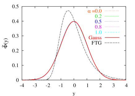
Figure 1: Results for the MRH_I distribution from simulations, plotted using $\sigma$-scaling (Eqs.(30) and (31)), for $\alpha$ in the range $0\leq\alpha\leq 1$. The simulations were performed with $N=4096$ terms in the Fourier series (24). The exact analytical result (32) for $N\to\infty$ (normalized Gaussian) is also shown, and the simulation results are within the linewidth of the Gaussian. The curve FTG corresponds to the Fisher-Tippett-Gumbel distribution, which is the limiting MRH_A distribution in the interval $0\leq\alpha<1$.

The simulation results shown in Fig. 1 will be discussed in the next Section. It turns out that the MRH_I distribution has the Gaussian form (32) not just for $\alpha=0$, but throughout the interval $0\leq\alpha\leq 1$.

IV.2 Special case $\alpha=2$

As mentioned after Eq. (27), the correlated Gaussian signals defined in the preceding Section correspond, for $\alpha=2$, $N\to\infty$, to random walks $h(t)$ governed by the stochastic equation of motion (26). The statistical weight or propagator $Z(h,h_{0},t)$ for a random walk from initial position $h_{0}$ to $h$ in a time $t$ satisfies the diffusion equation $\left(\partial/\partial t-D\thinspace\partial^{2}/\partial h^{2}\right)Z=0$, with initial condition $Z(h,h_{0},0)=\delta(h-h_{0})$. We set $D={1/2}$ from now on, corresponding to Gaussian signals normalized as in the preceding Section. The particular value of $D$ is not important, as it drops out of the MRH_I distribution on scaling by the average, as in Eqs. (28) and (29).

We will need the well known solutions of the diffusion equation

$$Z_{0}(h,h_{0},t)={1\over(2\pi t)^{1/2}}\exp\left[-(h-h_{0})^{2}/2t\right]\;$$ (33)

for random walks in the unbounded space $-\infty<h<\infty$, and

$$Z_{1}(h,h_{0},t)=Z_{0}(h,h_{0},t)-Z_{0}(h,-h_{0},t)$$ (34)

for random walks in the half space $h>0$, with an absorbing boundary absorbingboundary at $h=0$.

Let us consider the family of random walks $h(t)$ in the unbounded space $-\infty<h<\infty$ which satisfy the periodic boundary condition $h(0)=h(T)$. With no loss of generality in the result for the MRH_I distribution, one may choose $h(0)=0$. The fraction ${\cal F}_{\rm per}(m,T)$ of the walks with endpoints $h(0)=h(T)=0$ which never exceed height $m$ in the interval $0<t<T$ may be expressed as

$${\cal F}_{\rm per}(m,T) = {Z_{h<m}(0,0,T)\over Z_{0}(0,0,T)}$$ (35)

$$= {Z_{1}(m,m,T)\over Z_{0}(0,0,T)}=1-e^{-2m^{2}/T}\;.$$

Here $Z_{0}$ and $Z_{1}$ are the whole and half-space propagators of Eqs. (33) and (34), and $Z_{h<m}(h_{1},h_{0},T)$ is the propagator for random walks from $h_{0}$ to $h_{1}$ in time $T$ which lie entirely in the subspace $h<m$. In going from the first line of Eq. (35) to the second, we have used the relation $Z_{h<m}(h_{1},h_{0},T)=Z_{1}(m-h_{1},m-h_{0},T)$, which follows from invariance of the statistical weight under the coordinate transformation $h\to m-h$.

Differentiating ${\cal F}_{\rm per}(m,T)$ in Eq. (35) with respect to $m$ yields the MRH_I distribution

$$P_{\rm per}(m,T)={4m\over T}\thinspace e^{-2m^{2}/T}\\$$ (36)

for random walks with periodic boundary conditions. The mean value of the MRH_I distribution (36) is $\langle m\rangle=(\pi T/8)^{1/2}$. In terms of the variables $x=m/\langle m\rangle$ and $\Phi(x)=\langle m\rangle P_{\rm per}(m,T)$ of Eqs. (28) and (29), the distribution takes the form

$$\Phi_{\rm I}(x)=\frac{\pi}{2}\thinspace xe^{-\pi x^{2}/4}\;.$$ (37)

The mean value $\langle m\rangle$ of the MRH_I distribution given in the preceding paragraph is the same as the mean value $\langle h_{m}\rangle$ of the MRH_A distribution for $\alpha=2$ obtained by Majumdar and Comtet mc . The equality

$$\langle m\rangle=\langle h_{m}\rangle$$ (38)

is a general consequence of the definitions $m={\rm max}_{t}[h(t)-h(0)]$, $h_{m}={\rm max}_{t}[h(t)-\overline{h}]$, where $\overline{h}$ is the time average of $h(t)$, and time-translational invariance, on averaging over all paths, in the form $\langle h(0)\rangle=\langle\overline{h}\rangle$. Note that the equality (38) holds for all $\alpha$, not just $\alpha=2$, and for non-periodic as well as periodic boundary conditions, as long as the boundary conditions are consistent with the time translational invariance.

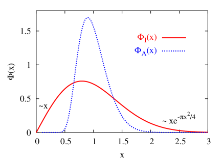
Figure 2: The exact MRH_I distribution (37) for $\alpha=2$ and periodic boundary conditions, and the corresponding MRH_A or Airy distribution mc . Both distributions are scaled with the average, as in Eqs. (28) and (29).

As in the case $\alpha=0$, the MRH_I and MRH_A distributions for $\alpha=2$ are not the same. Majumdar and Comtet mc have shown that for random walks with periodic boundary conditions, the MRH_A distribution is the so-called Airy distribution. The two distributions are compared in Fig. 2. We see that, for both small and large $x$, $\Phi_{\rm I}(x)$ has the greater weight. These features are found for all $\alpha>1$ and can be understood heuristically as follows:

In the case of $\Phi_{\rm A}(x)$, small $x$ means small $h_{m}=h_{\rm max}-\overline{h}$, or $h_{\rm max}\approx\overline{h}$. There are very few such configurations, only those for which $h(t)$ is nearly constant. In the case of $\Phi_{\rm I}(x)$, on the other hand, small $x$ means small $m=h_{\rm max}-h(0)$, or $h_{\rm max}\approx h(0)$. This condition is far less restrictive, since it is satisfied by any configuration $h(t)$ which is below $h(0)$ most of the time. Thus, small $m$ is much more probable than small $h_{m}$, i.e., $\Phi_{I}(x)\gg\Phi_{\rm A}(x)$ for small $x$.

Turning to the large $x$ behavior, we note that for a configuration $h(t)$ which makes a very large positive excursion with respect to the initial height $h(0)$, the average height $\overline{h}$ also tends to be much larger than $h(0)$. Thus, for such a configuration $m\gg h_{m}$. Roughly speaking, this means that a large value of $h_{m}$ has the same probability as a much larger value of $m$. This, together with a probability distribution that decreases rapidly with increasing $m$ implies $\Phi_{\rm I}(x)\gg\Phi_{\rm A}(x)$ for large $x$, as seen in Fig. 2.

The distribution of the maximum height not only depends on the reference height from which it is measured. It also depends on the boundary conditions imposed on $h(t)$ at $t=0$ and $t=T$. Before leaving the special case $\alpha=2$, we derive the MRH_I distribution for random walks for two non-periodic boundary conditions of general interest.

Consider the family of random walks $h(t)$ on the infinite interval $-\infty<h<\infty$ with fixed endpoints $h(0)=0$ and $h(T)=h_{1}$. For this fixed boundary condition Eqs. (35) and (36) are replaced by

$${\cal F}_{\rm fix}(m,h_{1};T) = {Z_{h<m}(h_{1},0,T)\over Z_{0}(h_{1},0,T)}$$ (39)

$$= {Z_{1}(m-h_{1},m,T)\over Z_{0}(h_{1},0,T)}=1-\exp\left[{h_{1}^{2}-(2m-h_{1})^{2}\over 2T}\right]\;.$$

and

$$P_{\rm fix}(m,h_{1};T)={2(2m-h_{1})\over T}\thinspace\exp\left[{h_{1}^{2}-(2m-h_{1})^{2}\over 2T}\right]\;,$$ (40)

which reduces to Eq. (36) for $h_{1}=0$.

Finally, we consider the family of random walks $h(t)$, $0<t<T$, with initial condition $h=0$ at $t=0$ but with no restrictions on $h(T)$. For this boundary condition Eqs. (35) and (36) are replaced by

$${\cal F}_{\rm free}(m,T) = {\int_{-\infty}^{m}dh_{1}\thinspace Z_{h<m}(h_{1},0,T)\over\int_{-\infty}^{\infty}dh_{1}\thinspace Z_{0}(h_{1},0,T)}=\int_{-\infty}^{m}dh_{1}\thinspace Z_{1}(m-h_{1},m,T)$$ (41)

$$= \int_{0}^{\infty}dh\thinspace Z_{1}(h,m,T)={\rm erf}\left({m\over\sqrt{2T}}\right)\;,$$ (42)

where ${\rm erf}$ denotes the error function as . The quantity ${\cal F}_{\rm free}(m,T)$ is the probability that a random walk which begins at the origin has not yet reached point $m$ after a time $T$. The integral on the right-hand side of Eq. (42) is the “persistence” probability that a random walk which begins at point $m$ has not yet reached the origin after a time $T$. Equation (42) states the obvious fact that these two probabilities are equal and reproduces the well known $T^{-1/2}$ decay of the persistence probability for long times.

Differentiating ${\cal F}_{\rm free}(m,T)$ in (42) with respect to $m$ yields the MRH_I distribution

$$P_{\rm free}(m,T)=\left({2\over\pi T}\right)^{1/2}\thinspace e^{-m^{2}/2T}\;.$$ (43)

After scaling by the average, as in Eqs. (28) and (29), with $\langle m\rangle=(2T/\pi)^{1/2}$, the distribution function (43) takes the form

$$\Phi_{\rm I}(x)={2\over\pi}\thinspace e^{-x^{2}/\pi}\;,$$ (44)

which is clearly different from the result (37) for periodic boundary conditions.

IV.3 Special case $\alpha=4$

As pointed out below Eq. (27), the correlated Gaussian signal $h(t)$ of Sec. III may be interpreted, for $\alpha=4$, $N\to\infty$, as the position of a particle which is randomly accelerated according to the stochastic equation of motion (26). Following the same approach as in the preceding Subsection, we work with the statistical weight or propagator $Z(h,v;h_{0},v_{0};t)$ for a randomly-accelerated particle with position and velocity $h_{0},v_{0}$ at $t=0$ and values $h,v$ at a later time $t$. This quantity satisfies the Fokker-Planck equation $\left(\partial/\partial t+v\partial/\partial h-{\cal D}\thinspace\partial^{2}/\partial v^{2}\right)Z=0$, which is basically a diffusion equation for the velocity, with initial condition $Z(h,v;h_{0},v_{0};0)=\delta(h-h_{0})\delta(v-v_{0})$. We set ${\cal D}=1$ from now on, as in Ref. twb93 . The particular value of ${\cal D}$ is not important, as it drops out of the MRH_I distribution on scaling by the average, as in Eqs. (28) and (29).

In calculating the MRH_I distribution, we will need the solutions $Z_{0}$ and $Z_{1}$ to the Fokker-Planck equation in the unbounded space $-\infty<h<\infty$ and in the half space $h>0$, with an absorbing boundary condition absorbingboundary , respectively. Expressions for $Z_{0}(h,v;h_{0},v_{0};t)$ and for the Laplace transform $\tilde{Z}_{1}(h,v;h_{0},v_{0};s)=\int_{0}^{\infty}dt\thinspace e^{-st}Z_{1}(h,v;h_{0},v_{0};t)$ are given in Ref. twb93 and in Appendix A of this paper.

Let us consider the family of trajectories $h(t)$ in the unbounded space $-\infty<h<\infty$ with periodicity $h(t)=h(t+T)$. As in the case $\alpha=2$, we may choose $h(0)=0$, with no loss of generality in the result for the MRH_I distribution. The velocities at $t=0$ and $T$ are the same, as follows from the periodicity, but otherwise unrestricted. All values of the initial velocity are assumed to be equally probable. For this boundary condition, Eq. (35) in our treatment of the random walk is replaced by

$${\cal F}_{\rm per}(m,T) = {\int_{-\infty}^{\infty}dv\thinspace Z_{h<m}(0,v;0,v;T)\over\int_{-\infty}^{\infty}dv\thinspace Z_{0}(0,v;0,v;T)}$$ (45)

$$= {\int_{-\infty}^{\infty}dv\thinspace Z_{1}(m,v;m,v;T)\over\int_{-\infty}^{\infty}dv\thinspace Z_{0}(0,v;0,v;T)}.$$

Here $Z_{h<m}(h_{1},v_{1};h_{0},v_{0};T)$ is the statistical weight for a randomly accelerated particle that propagates from point $h_{0},v_{0}$ in phase space to $h_{1},v_{1}$ in a time $T$ without leaving the half space $h<m$. In going from the first line of Eq. (45) to the second, we have used the relation $Z_{h<m}(h_{1},v_{1};h_{0},v_{0};T)=Z_{1}(m-h_{1},-v_{1};m-h_{0},-v_{0};T)$, which follows from invariance of the statistical weight under the coordinate transformation $h\to m-h$. The probability distribution of $m$ is obtained by differentiating ${\cal F}_{\rm per}(m,T)$ with respect to $m$.

Using the results for $Z_{0}$ and $Z_{1}$ in Ref. twb93 , we have derived the MRH_I distribution for the periodic boundary condition of the preceding paragraph. The calculation is outlined in Appendix A. For the mean value, one obtains $\langle m\rangle={1\over 24}\left(\pi T^{3}\right)^{1/2}$. In terms of the scaling variable $x$ and scaling function $\Phi(x)$ of Eqs. (28) and (29), the distribution is given by

$$\Phi_{\rm I}(x)=2^{-2/3}3^{1/6}\pi^{-1/6}\thinspace x^{-1/3}\thinspace\exp\left(-\frac{\pi}{12}\thinspace x^{2}\right)U\left(-\frac{1}{6},\frac{2}{3},\frac{\pi}{12}\thinspace x^{2}\right)\;,$$ (46)

where $U(a,b,z)$ is Kummer’s function as . The function $\Phi_{\rm I}(x)$ shown in Fig. 3 has the asymptotic forms as

$$\Phi_{\rm I}(x)\approx\left\{\begin{array}[]{l}2^{-4/3}3^{1/6}\pi^{-2/3}\Gamma({2\over 3})\thinspace x^{-1/3}\;,\\ {1\over 2}\exp\left(-\thinspace{\pi\over 12}x^{2}\right)\;,\end{array}\right.\quad\begin{array}[]{l}x\to 0\;,\\ x\to\infty\;,\end{array}$$ (47)

and the moments

$$\langle x^{\nu}\rangle={\Gamma({3\over 2}\nu+1)\over\Gamma(\nu+1)}\thinspace\Gamma(\textstyle{5\over 2})^{-\nu}\;,$$ (48)

for arbitrary $\nu>-2/3$.

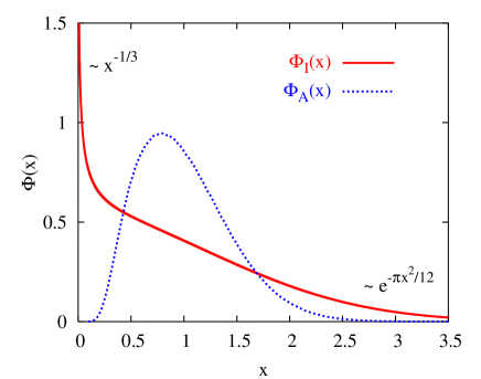
Figure 3: The exact MRH_I distribution (46) for $\alpha=4$ and periodic boundary conditions, and the corresponding MRH_A distribution, determined from simulations gyorgyietal . Both distributions are scaled with the average, as in Eqs. (28) and (29). The asymptotic forms of the MRH_I distribution for small and large $x$ are given in Eq. (47). The MRH_A distribution is exponentially small for small $x$ and for large $x$ is essentially Gaussian with a smaller variance gyorgyietal .

The difference between $\Phi_{\rm I}(x)$ and $\Phi_{\rm A}(x)$ in Fig. 3 is even more dramatic than for $\alpha=2$. For $\alpha=4$, $\Phi_{\rm I}(x)$ diverges at $x=0$ and decreases monotonically with increasing $x$. The increasing weight, with increasing $\alpha$, of the MRH_I distribution $\Phi_{\rm I}(x)$ will be discussed below, in connection with simulation results for a broad range of $\alpha$.

Next, we consider the MRH_I distribution for a randomly accelerated particle with position $h=0$ and velocity $v_{0}$, but with no restrictions on the position and velocity at $t=T$. For this boundary condition Eqs. (41) and (42) are replaced by

$${\cal F}_{\rm free}(m,v_{0};T) = {\int_{-\infty}^{m}dh_{1}\int_{-\infty}^{\infty}dv_{1}\thinspace Z_{h<m}(h_{1},v_{1};0,v_{0};T)\over\int_{-\infty}^{\infty}dh_{1}\int_{-\infty}^{\infty}dv_{1}\thinspace Z_{0}(h_{1},v_{1};0,v_{0};T)}$$ (49)

$$= \int_{-\infty}^{m}dh_{1}\int_{-\infty}^{\infty}dv_{1}\thinspace Z_{1}(m-h_{1},-v_{1};m,-v_{0};T)$$ (50)

$$= \int_{0}^{\infty}dh\int_{-\infty}^{\infty}dv\thinspace Z_{1}(h,v;m,-v_{0};T)=q(m,-v_{0};T)\;.$$ (51)

Here ${\cal F}_{\rm free}(m,v_{0};T)$ is the probability that a randomly accelerated particle which begins at the origin with velocity $v_{0}$ has not yet reached point $m$ in a time $T$. As in the case $\alpha=2$, ${\cal F}_{\rm free}$ represents a “persistence” probability. The quantity $q(m,-v_{0};T)$ on the right-hand side of Eq. (51) is the probability that a randomly accelerated particle with initial position $m$ and initial velocity $-v_{0}$ has not yet reached the origin after a time $T$. Equation (51) states the obvious fact that these two probabilities are equal and reproduces (see Eq. (54) below) the well-known $T^{-1/4}$ decay twb93 of the persistence probability for long times.

Combining $P_{\rm free}(m,v_{0};T)=\partial_{\rm free}{\cal F}(m,v_{0};T)/\partial m$, Eq. (51), and the expression for the Laplace transform of $q(m,-v_{0};T)$ in Eq. (19) of Ref. twb93 , we obtain

$$\tilde{P}_{\rm free}(m,v_{0};s) = \int_{0}^{\infty}dT\thinspace e^{-sT}P(m,v_{0};T)$$

$$= \int_{0}^{\infty}dF\thinspace F^{-2/3}e^{-Fm}{\rm Ai}\left(-F^{1/3}v_{0}+F^{-2/3}s\right)$$

$$\times \left[1+{1\over 4\pi^{1/2}}\Gamma\left(-\textstyle{1\over 2},{2\over 3}F^{-1}s^{3/2}\right)\right]$$ (53)

for the Laplace transform of the MRH_I distribution. Here ${\rm Ai}(z)$ and $\Gamma(a,z)$ are the standard Airy and incomplete Gamma function. In principle, $P_{\rm free}(m,v_{0},T)$ can be determined from Eq. (53) by integrating over $F$ and inverting the Laplace transform numerically. For $v_{0}=0$ all of the moments $\langle m^{\nu}\rangle$ of the distribution can be calculated analytically twbunpub from Eq. (53). Equation (21) of Ref. twb93 leads to the exact asymptotic form

$$P_{\rm free}(m,v_{0};T) = 2^{-1}3^{4/3}\pi^{-3/2}\Gamma(\textstyle{1\over 4})$$ (54)

$$\times {\partial\over\partial m}\left[\left(m^{2}\over T^{3}\right)^{1/12}U\left(-{1\over 6},{2\over 3},\thinspace-{v_{0}^{3}\over 9m}\right)\right]\;,$$

for $T\gg m^{2/3}$ and $T\gg|v_{0}|^{1/2}$. Here $U(a,b,z)$ is Kummer’s function as .

Finally, we note that the MRH_I distribution for $\alpha=4$ and all its moments can be calculated analytically twbunpub for two additional boundary conditions: In the first case $h(T)=h(0)$ and $v(T)=v(0)=0$. In the second case $h(T)=h(0)$, while $v(T)$ and $v(0)$ are independent and unrestricted, and integrated over all values between $-\infty$ and $\infty$.

IV.4 Special case $\alpha=\infty$

According to Eqs. (22)-(24), all but the modes with Fourier coefficients $c_{-1}$ and $c_{1}$ are suppressed in the limit $\alpha\to\infty$, so that

$$h(t)-h(0) = c_{1}\left(e^{2\pi it/T}-1\right)+c_{1}^{*}\left(e^{-2\pi it/T}-1\right)$$ (55)

$$= 2|c_{1}|\left[\cos\left(2\pi t/T+\varphi\right)-\cos\varphi\right]\;,$$ (56)

where $c_{1}=|c_{1}|e^{i\varphi}$. Thus, $m={\rm max}_{t}[h(t)-h(0)]=2|c_{1}|(1-\cos\varphi)=4|c_{1}|\sin^{2}(\varphi/2)$, and, in accordance with Eqs. (22) and (23), the distribution of $m$ is given by

$$P(m,N) = {\lambda\over\pi}\int_{0}^{2\pi}d\varphi\int_{0}^{\infty}d|c_{1}|\thinspace|c_{1}|e^{-\lambda|c_{1}|^{2}}\delta\left(m-4|c_{1}|\sin^{2}{\varphi\over 2}\right)\;,$$ (57)

$$= {\lambda m\over 8\pi}\int_{0}^{\pi}d\vartheta\thinspace(\sin\vartheta)^{-4}\exp\left(-{\lambda m^{2}\over 16\sin^{4}\vartheta}\right)\;.$$ (58)

Here we have absorbed several constants in $\lambda$, rewritten the integral $\int_{-\infty}^{\infty}d\thinspace{\rm Re}\left[c_{1}\right]\int_{-\infty}^{\infty}d\thinspace{\rm Im}\left[c_{1}\right]$ over phase space (see Eq. (27)) in terms of polar coordinates $(|c_{1}|$, $\varphi)$, performed the integration over $|c_{1}|$, and made the substitution $\vartheta={1\over 2}\varphi$. By carrying out the $m$ integration before the $\vartheta$ integration, it is easy to check that $P(m,N)$ in Eq. (58) satisfies the normalization condition $\int_{0}^{\infty}dm\thinspace P(m,N)=1$ and has the average value $\langle m\rangle=(\pi/\lambda)^{1/2}$.

The integral over $\vartheta$ in Eq. (58) can be evaluated with the help of Ref. gr or Mathematica. In terms of the variable $x=m/\langle m\rangle=(\lambda/\pi)^{1/2}m$ and scaling function $\Phi(x)$ of Eqs. (28) and (29), the MRH_I distribution for periodic boundary conditions and $\alpha=\infty$ takes the form

$$\Phi_{\rm I}(x)=2^{-3/2}\left({\pi x^{2}\over 16}\right)^{-1/4}\exp\left(-\thinspace{\pi x^{2}\over 16}\right)U\left(-{1\over 4},{1\over 2},{\pi\over 16}\thinspace x^{2}\right)\;,$$ (59)

where again $U(a,b,z)$ is Kummer’s function as . The function $\Phi_{\rm I}(x)$ has the asymptotic forms as

$$\Phi_{\rm I}(x)\approx\left\{\begin{array}[]{l}2^{-1}\pi^{-3/4}\Gamma({3\over 4})\thinspace x^{-1/2}\;,\\ 2^{-3/2}\exp\left(-\thinspace{\pi\over 16}x^{2}\right)\;,\end{array}\right.\quad\begin{array}[]{l}x\to 0\;,\\ x\to\infty\;,\end{array}$$ (60)

and the moments

$$\langle x^{\nu}\rangle={\Gamma({1\over 2}+\nu)\over\Gamma({1\over 2}+{\nu\over 2})}\thinspace\Gamma(\textstyle{3\over 2})^{-\nu}\;$$ (61)

for arbitrary $\nu>-{1\over 2}$.

From Eq. (60) we see that MRH_I distribution function (59) diverges as $x^{-1/2}$ for $x\to 0$, even more strongly than in the case $\alpha=4$ (see Eq. (47)), where there is an $x^{-1/3}$ divergence. The distribution function (59) is plotted in Fig. 4. The MRH_A distribution for $\alpha=\infty$, calculated by Györgyi et al. gyorgyietal , has precisely the same form (37) as the MRH_I distribution for $\alpha=2$. Thus, the curves $\alpha=2$ and $\infty$ in Fig. 4 correspond to the MRH_A and MRH_I distributions, respectively, for $\alpha=\infty$.

V Results of simulations

In addition to the analytical results for the special values of $\alpha=0,2,4$ and $\infty$, we have determined the MRH_I distribution for intermediate values of $\alpha$ by numerical simulations, following the procedure described in Sec. III. This allows us to address some interesting questions concerning the $\alpha$ dependence. In the simulations the number $N$ of terms in the Fourier series (24) was chosen large enough so that finite-size effects were negligible, and the exact results of the preceding Section, corresponding to $N=\infty$, could be reproduced with “width-of-the-line” accuracy everywhere except in the immediate neighborhood of $x=0$, where $\Phi_{\rm I}(x)$ diverges for $\alpha$ greater than a critical value close to 3.

First we turn to the weak-correlation regime $0<\alpha<1$, where the correlation function $\langle h(0)h(t)\rangle$ remains finite in the limit $T\to\infty$ with $t/T$ finite, decaying with power law $t^{\alpha-1}$ gyorgyietal . Berman Berman-1964 has proved that in this regime the correlations are too weak to affect the MRH_A distribution, which has the same FTG form as for $\alpha=0$. According to the simulation results shown in Fig. 1, the MRH_I distribution has the same Gaussian form (32) throughout the interval $0\leq\alpha<1$. Thus, the correlations appear to be equally irrelevant for the MRH_I distribution.

At $\alpha=1$ we enter a regime of stronger correlations. The correlation function $\langle h(0)h(t)\rangle$ diverges as $\ln T$ at $\alpha=1$ and as $T^{\alpha-1}$ for $\alpha>1$. Although Berman’s result on the irrelevance of correlations no longer holds at $\alpha=1$, the numerically determined MRH_I distribution is still in good agreement with the Gaussian form (32).

Once we are well within the strongly correlated regime ($\alpha$ larger than $\sim 1.2$), the convergence with increasing $N$ is much faster than for $\alpha<1$, just as in the case of the MRH_A distribution gyorgyietal . Our exact and numerical results MRH_I for $\alpha>1$ are summarized in Fig. 4.

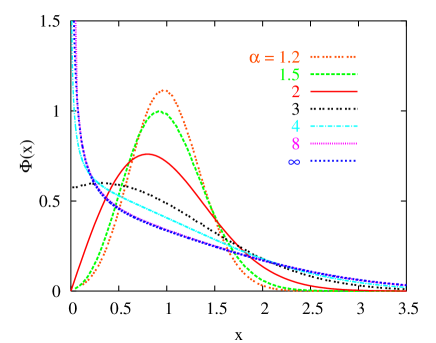
Figure 4: MRH_I distribution for periodic boundary conditions and $\alpha$ in the range $1.2\leq\alpha<\infty$, scaled with the average, as in Eqs. (28) and (29). For $\alpha=2,\,4$ and $\infty$ the exact analytic results are shown, while the results for $\alpha=1.2,\,1.5,\,3$ and $8$ were obtained from simulations with $N=4096$ terms in the Fourier series (24). Note that the curves for $\alpha=8$ and $\alpha=\infty$ are practically indistinguishable.

A prominent feature in Fig. 4, which we have already mentioned, is the increase in weight, with increasing $\alpha$ of the distribution function $\Phi_{\rm I}(x)$ for small $x$, with a divergence at $x=0$ for $\alpha$ greater than a critical value $\alpha_{c}$. For small $x$,

$$\Phi_{\rm I}(x)\sim x^{\gamma(\alpha)}\;,\quad x\to 0\;,$$ (62)

with an exponent $\gamma(\alpha)$ that decreases monotonically as $\alpha$ increases, and changes from positive to negative at $\alpha_{c}$. The Gaussian form of $P(m,N)$ for $0\leq\alpha<1$, with $\langle m\rangle_{N}\sim\sigma_{N}^{-1}\sim(\ln N)^{1/2}$, leads to $\Phi_{\rm I}(x)=\delta(x-1)$ on scaling by the average. This is consistent with $\gamma(\alpha)=\infty$ for $\alpha<1$ in Eq. (62). The exact results in Eqs. (37), (46), and (60) imply $\gamma(2)=1$, $\gamma(4)=-{1\over 3}$, and $\gamma(\infty)=-{1\over 2}$. The curve for $\alpha=3$ in Fig. 4 looks compatible with $\alpha_{c}=3$, but determining $\alpha_{c}$ numerically with good precision requires a more extensive study, with careful attention to finite size effects near $x=0$ and $\alpha=3$.

We have also studied the small $x$ singularity for $\alpha=5$ and $6$ numerically. In both cases the exponents $\gamma$ are in good agreement with the value $-{1\over 2}$, although the simulations can, of course, not exclude small deviations. These findings and the exact analytical results $\gamma(4)=-{1\over 3}$ and $\gamma(\infty)=-{1\over 2}$ appear to indicate that $\gamma(\alpha)=-{1\over 2}$ for all $\alpha>\alpha_{u}$, where $\alpha_{u}$ is an upper critical value between 4 and 5. In the next Section we present some simple physical arguments which predict $\alpha_{c}=3$ and $\alpha_{u}=5$. We also obtain a formula for $\gamma(\alpha)$, $\alpha\leq 5$ which reproduces all the known exact values and agrees with the simulations.

VI Connection between the MRH_I distribution and the density of states near extremes

As we saw at the end of Sec. II, for iid variables the density of states near extremes, studied by Sabhapandit and Majumdar sm , and the MRH_I distribution are identical. Here we show that this equivalence continues to hold for correlated variables, as long as the probability distribution of the signals is time-translationally invariant. This is the case for correlated Gaussian signals with $1/f^{\alpha}$ noise and periodic boundary conditions, and we use the equivalence with the density of states to study the small $x$ singularity of $\Phi_{\rm I}(x)$.

In a time-translationally invariant system, all of the points traced out by the signal correspond to possible initial states. For a given realization of the signal, the distribution of heights measured from the maximum height is the same as the the distribution of the maximum height with respect to all these possible initial heights. Thus, averaging over all realizations yields identical distributions for the quantities $h_{\rm max}-h$ and $h_{\rm max}-h(0)$. We have checked the equivalence of the two distributions for periodic, correlated Gaussian signals both numerically and, for $\alpha=$ 2 and 4, by expressing both distributions in terms of propagators.

We now present a simple picture that is very helpful in understanding the threshold behavior of the density of states relative to the maximum. The idea is most readily understood in the $\alpha\to\infty$ limit. In this case, considered in Sec. IV.4, each path is a smooth curve with a parabolic maximum, so that $\delta h=h(t_{m})-h(t)\sim(\delta t)^{2}$, where $\delta t=t-t_{m}$. Thus, the density of states relative to the maximum has the singularity $\rho(\delta h)\sim\delta t/\delta h\sim(\delta h)^{-1/2}$ for $\delta h\to 0$. Since the density of states is the same as the MRH_I distribution, the exponent $\gamma$ in Eq. (62) has the value $-{1\over 2}$, in agreement with the exact result in Eq. (60).

As long as the path $h(t)$ is smooth near its maximum, in the sense that typical maxima are parabolic, the above argument applies. Since the average increments of $1/f^{\alpha}$ signals scale as

$$|\delta h|\sim\sqrt{\langle\delta h^{2}\rangle}\sim|\delta t|^{(\alpha-1)/2}$$ (63)

for $\alpha>1$, the signals are expected to be twice differentiable for $\alpha\geq 5$. Thus, we predict $\gamma=-{1\over 2}$ for $\alpha\geq\alpha_{u}=5$, in agreement with the simulations for $\alpha=$5 and 6.

The lower critical value $\alpha_{c}$ is the smallest value of $\alpha$ for which the $1/f^{\alpha}$ signals are once differentiable, which, according to the scaling (63) is expected to be $\alpha_{c}=3$. In this case, the paths near the maximum are basically rooftop-like, so that $\delta h\sim|\delta t|$ and $\rho\sim$ constant. This implies $\gamma(3)=0$, which is compatible with the simulation results for $\alpha=3$ in Fig. 4.

To obtain a formula for $\gamma(\alpha)$ in the interval $1\leq\alpha\leq 5$, we assume that the scaling behavior in Eq. (63) applies near the maximum of the paths. This implies $\rho(\delta h)\sim\delta t/\delta h\sim(\delta h)^{(3-\alpha)/(\alpha-1)}$ and so $\gamma(\alpha)=(3-\alpha)/(\alpha-1)$.

In summary, the simple scaling picture predicts the small argument behavior

$$\rho(\delta h)\sim\delta h^{\gamma}\;,\quad\Phi_{\rm I}(x)\sim x^{\gamma}\;,$$ (64)

where

$$\gamma(\alpha)=\begin{cases}\displaystyle\frac{3-\alpha}{\alpha-1}\;,&\alpha<5\;,\\ \displaystyle-\frac{1}{2}\;,&\alpha\geq 5\;,\end{cases}$$ (65)

for both the density of near extreme states and the MRH_I distribution. The above derivation may seem oversimplified, but the result is in remarkable agreement with those presented in Secs. IV and V. Expression (65) reproduces the exact values of $\gamma(\alpha)$ for $\alpha=$2, 4, and $\infty$ collected below Eq. (62). Furthermore, the divergence $\gamma\to\infty$ for $\alpha\to 1$ is in accordance with the fact that, in this limit, the MRH_I distribution approaches a delta function centered at $x=1$. It also agrees with all our simulations. We note, however, that a convincing numerical confirmation of $\gamma(\alpha)$ was not achieved in the regime $1<\alpha\leq 1.6$ due to finite-size corrections. We suspect the relation (65) is exact, but more effort is needed to put it on a firmer foundation.

The equivalence of the MRH_I distribution and the density of near-extreme states and the scaling picture presented above furnish a simple physical explanation for the striking increase of both distributions, for small relative heights, with increasing $\alpha$. As $\alpha$ increases, high frequency Fourier components of the Gaussian signal are suppressed. Typical signals become smoother and approach the maximum height less steeply, remaining close to the maximum for a longer time. Beyond $\alpha=3$ the approach to the maximum is basically tangential, becoming parabolic for $\alpha>5$. Thus, the density of near maximum heights $\delta t/\delta h$ increases as $\alpha$ increases and diverges at the maximum for $\alpha>3$. A large density of near-maximum heights is equivalent to a high probability that the maximum height is close to the initial height. The scaling picture provides both a simple qualitative explanation of the singular small-argument behavior Eq. (64) of the two equivalent distributions $\rho(\delta h)$ and $\Phi_{\rm I}(x)$ and a quantitatively accurate prediction for the exponent $\gamma(\alpha)$.

VII Concluding remarks

In this paper we have shown the importance of the reference point from which the maximum is measured in extreme statistics. We found that the distributions of the maximum height relative to the average height and relative to the initial height are generally not the same. One reason for this is that both the average height and the initial height are fluctuating quantities, but the distributions of their fluctuations are different. Furthermore, the two different reference heights impose different constraints on the paths consistent with a particular value of the maximum height. For example, the probability for small maximum height relative to the average height is small, since only paths which remain close to the average for the duration of the signal contribute. In the case of a small height relative to the initial height, a much larger family of paths, which remain below the initial height most of the time, is allowed. This difference is highlighted by the analytical result that the MRH_A distribution has an essential singularity at small heights with exponentially suppressed values gyorgyietal , whereas the MRH_I distribution has power law behavior near the origin.

A notable feature of the aforementioned singularity of the MRH_I distribution is that the exponent in the power law monotonically decreases with $\alpha$, thus increasing the weight near zero heights. This is in agreement with known persistence properties of $1/f^{\alpha}$ processes Bray-Maj-2001 , where the weight of configurations persisting below the starting height shows a similar trend in $\alpha$. To make this intuitively appealing connection more rigorous, further considerations would be required.

The small height singularity of the MRH_I distribution was described quantitatively with the help of a remarkable connection to the density of near extreme states. Namely, we found that they are identical for iid variables or, more generally, for signals drawn from time-translationally invariant distributions. It should be noted that we also considered boundary conditions other than periodic, with the aim of illustrating the dependence of boundary conditions on the extreme statistics. Since time-translational invariance is violated in these cases, the density of near extreme states remains open for further studies.

Appendix A Derivation of results for $\alpha=4$

In the case $\alpha=4$, corresponding to random acceleration, the free space and half space propagators $Z_{0}$ and $Z_{1}$ are given by twb93

$$Z_{0}(h,v;h_{0},v_{0};T) = 3^{1/2}(2\pi)^{-1}t^{-2}$$ (66)

$$\times \exp\left\{-3t^{-3}\left[(h-h_{0}-vt)(h-h_{0}-v_{0}t)+{1\over 3}(v-v_{0})^{2}t^{2}\right]\right\}$$

$$Z_{1}(h,v;h_{0},v_{0};T) = Z_{0}(h,v;h_{0},v_{0};T)+\Delta(h,v;h_{0},v_{0};T)\;,$$ (67)

$$\tilde{\Delta}(h,v;h_{0},v_{0};s) = -{1\over 2\pi}\int_{0}^{\infty}{dF\over F^{1/6}}\int_{0}^{\infty}{dG\over G^{1/6}}$$ (68)

$$\times {\exp\left[-(Fh+Gh_{0})-{2\over 3}s^{3/2}\left(F^{-1}+G^{-1}\right)\right]\over F+G}$$

$$\times {\rm Ai}\left(-F^{1/3}v+F^{-2/3}s\right){\rm Ai}\left(G^{1/3}v_{0}+G^{-2/3}s\right)\;.$$

Here $\tilde{\Delta}(\dots;s)$ denotes the Laplace transform ${\cal L}\thinspace\Delta(\dots;T)=\int_{0}^{\infty}dT\thinspace e^{-sT}\Delta(\dots;T)$, and ${\rm Ai}(z)$ is the standard Airy function ${\rm Ai}$ as . Using these results, we rewrite Eq. (45) in the form

$${\cal F}_{\rm per}(m,T)=1+2\sqrt{\pi}T^{3/2}{\cal L}^{-1}\int_{-\infty}^{\infty}dv\thinspace\tilde{\Delta}(m,v;m,v;s)\;,$$ (69)

where ${\cal L}^{-1}$ indicates the inverse Laplace transform.

It is convenient to calculate the moments

$$\langle m^{\nu}\rangle=\int_{0}^{\infty}dm\thinspace m^{\nu}{\partial\over\partial m}{\cal F}_{\rm per}(m,T)\;,$$ (70)

which have simple Laplace transforms, and then construct the extreme distribution from the moments. After substituting Eqs. (68) and (69) into (70), we first integrate over $m$ and then over $v$, using

$$\int_{-\infty}^{\infty}dv\thinspace{\rm Ai}\left(-F^{1/3}v+F^{-2/3}s\right){\rm Ai}\left(G^{1/3}v+G^{-2/3}s\right)=$$

$$\qquad\qquad\qquad(F+G)^{-1/3}{\rm Ai}\left[s\left(F^{-1}+G^{-1}\right)^{2/3}\right]\;,$$ (71)

which follows from the integral representation (10.4.32) of ${\rm Ai}(z)$ in Ref. as . On expressing the right-hand side of Eq. (71) in terms of the Bessel function $K_{1/3}(y)$ according to Eq. (10.4.14) of Ref. as , making the changes of variables $G=Fz$, $F={2\over 3}s^{3/2}y^{-1}(1+z^{-1})$, integrating over $y$ and $z$ with the help of Ref. gr and Mathematica, and using ${\cal L}^{-1}\left[s^{-\alpha-1}\right]=\Gamma(\alpha+1)^{-1}T^{\alpha}$, one obtains

$$\langle m^{\nu}\rangle={\Gamma({3\over 2}\nu+1)\over\Gamma(\nu+1)}\left({T^{3/2}\over 18}\right)^{\nu}={\Gamma({3\over 2}\nu+1)\over\Gamma(\nu+1)}\left[\Gamma\left(\textstyle{5\over 2}\right)^{-1}\langle m\rangle\right]^{\nu}\;,$$ (72)

which implies the scaled moments (48).

To calculate $P_{\rm per}(m,T)$, we consider the Laplace transform or generating function

$$\hat{P}_{\rm per}(\xi,T)=\int_{0}^{\infty}dm\thinspace e^{-\xi m}P_{\rm per}(m,T)=\sum_{n=0}^{\infty}{\langle m^{n}\rangle\over n!}(-\xi)^{n}\;,$$ (73)

Substituting Eq. (72) into (73) and carrying out some straightforward steps, one obtains

$$\hat{P}_{\rm per}(\xi,T) = \sum_{n=0}^{\infty}{\Gamma({3\over 2}n+1)\over\Gamma(n+1)^{2}}\left[-\Gamma\left(\textstyle{5\over 2}\right)^{-1}\langle m\rangle\xi\right]^{n}\;,$$ (74)

$$= \int_{0}^{\infty}dx\thinspace e^{-x}\sum_{n=0}^{\infty}{1\over\Gamma(n+1)^{2}}\left[-\Gamma\left(\textstyle{5\over 2}\right)^{-1}\langle m\rangle\xi x^{3/2}\right]^{n}\;,$$ (75)

$$= \int_{0}^{\infty}dx\thinspace e^{-x}J_{0}\left(2\sqrt{\Gamma\left(\textstyle{5\over 2}\right)^{-1}\langle m\rangle\xi x^{3/2}}\right)\;,$$ (76)

$$= \xi^{-2/3}\int_{0}^{\infty}dy\thinspace\exp\left(-y\xi^{-2/3}\right)J_{0}\left(2\sqrt{\Gamma\left(\textstyle{5\over 2}\right)^{-1}\langle m\rangle y^{3/2}}\right)\;,$$ (77)

where $J_{0}(x)$ is the standard Bessel function as .

Next we will need the relation

$${\cal L}^{-1}\left[\xi^{-2/3}\exp\left(-y\xi^{-2/3}\right)\right]=m^{-1/3}H(m^{2/3}y)\;,$$ (79)

where

$$H(z)=\sum_{n=0}^{\infty}{(-z)^{n}\over\Gamma(n+1)\Gamma\left({2\over 3}n+{2\over 3}\right)}\;,$$ (80)

which follows from expanding the exponential function on the left-hand side of Eq. (79) in powers of $y\xi^{-2/3}$ and inverting the Laplace transform term by term. Evaluating the inverse Laplace transform of Eq. (77) using Eq. (79) and changing the integration variable to $z=m^{2/3}y$ yields

$$P_{\rm per}(m,T)=m^{-1}\int_{0}^{\infty}dz\thinspace H(z)J_{0}\left(2\sqrt{\Gamma\left(\textstyle{5\over 2}\right)^{-1}m^{-1}\langle m\rangle z^{3/2}}\right)\;.$$ (81)

With the help of Mathematica one may express the series (80) in terms of generalized hypergeometric functions gr and evaluate the integral (81). This leads to

$$H(z) = \Gamma\left(\textstyle{2\over 3}\right)^{-1}\thinspace_{0}F_{4}\left(\textstyle{{1\over 3},{1\over 3},{2\over 3},{5\over 6}};-{1\over 108}z^{3}\right)$$

$$- \Gamma\left(\textstyle{4\over 3}\right)^{-1}\thinspace z\;_{0}F_{4}\left(\textstyle{{2\over 3},{2\over 3},{7\over 6},{4\over 3}};-{1\over 108}z^{3}\right)$$

$$+ \textstyle{1\over 2}\thinspace z^{2}\;_{0}F_{4}\left(1,{4\over 3},{3\over 2},{5\over 3};-{1\over 108}z^{3}\right)$$

and our final result for the extreme distribution,

$$P_{\rm per}(m,T)=\langle m\rangle^{-1}\Phi_{\rm I}\left({m\over\langle m\rangle}\right)\;,$$ (83)

where $\Phi_{\rm I}(x)$ is given in Eq. (46).

References

- (1) R. Fisher and L. Tippett, Proc. Cambridge Philos. Soc. 24, 180 (1928).
- (2) B. Gnedenko, Ann. Math. 44, 423 (1943).
- (3) E. Gumbel Statistics of Extremes, (Dover, New York, 1958).
- (4) J. Galambos The Asymptotic Theory of Extreme Order Statistics, (Wiley, New York, 1978).
- (5) R. W. Katz, M. B. Parlange, and P. Naveau, Adv. Water Resour.25, 1287 (2002).
- (6) P. Embrechts, C. Klüppelberg, and T. Mikosch, Modelling Extremal Events for Insurance and Finance (Springer, Berlin, 2004).
- (7) A. R. Solow and J. M. Broadus, Climatic Change 15, 449 (1989).
- (8) J.-P. Bouchaud and M. Mézard, J. Phys. A 30, 7997 (1997).
- (9) S. Raychaudhuri, M. Cranston, C. Przybyla, and Y. Shapir, Phys. Rev. Lett. 87, 136101 (2001).
- (10) T. Antal, M. Droz, G. Györgyi, and Z. Rácz, Phys. Rev. Lett. 87, 240601 (2001).
- (11) G. Györgyi, P. C. W. Holdsworth, B. Portelli, and Z. Rácz, Phys. Rev. E 68 056116 (2003).
- (12) S. N. Majumdar and A. Comtet, Phys. Rev. Lett. 92, 225501 (2004), J. Stat. Phys. 119, 777 (2005).
- (13) C. J. Bolech and A. Rosso, Phys. Rev. Lett. 93, 125701 (2004).
- (14) H. Guclu and G. Korniss, Phys. Rev. E 69, 065104(R) (2004).
- (15) P. L. Krapivsky and S. N. Majumdar, Phys. Rev. Lett. 85, 5492 (2000).
- (16) A. Comtet, P. Leboeuf, and S. N. Majumdar, Phys. Rev. Lett. 98, 070404 (2007).
- (17) J. F. Eichner, J. W. Kantelhardt, A. Bunde, and S. Havlin, Phys. Rev. E 73, 016130 (2006).
- (18) S. Raychaudhuri, M. Cranston, C. Przybyla and Y. Shapir, Phys. Rev. Lett. 87, 136101 (2001).
- (19) G. Györgyi, N. R. Moloney, K. Ozogány, and Z. Rácz, Phys. Rev. E 75, 021123 (2007).
- (20) S. Sabhapandit and S. N. Majumdar, Phys. Rev. Lett. 98, 140201 (2007).
- (21) L. de Haan and S. Resnick, Ann. Probab. 24, 97 (1996).
- (22) T. Antal, M. Droz, G. Györgyi, and Z. Rácz, Phys. Rev. E 65 046140 (2002).
- (23) M. B. Weissman, Rev. Mod. Phys. 60, 537 (1988).
- (24) T. W. Burkhardt, J. Phys. A 26, L1157 (1993).
- (25) The absorbing boundary condition excludes random walks from which reach the boundary in propagating from to .
- (26) Handbook of Mathematical Functions, edited by M. Abramowitz and I. A. Stegun (Dover, New York, 1965).
- (27) I. S. Gradshteyn and E. M. Ryzhik, Tables of Integrals, Series, and Products (Academic, New York, 1980).
- (28) T. W. Burkhardt, unpublished.
- (29) S. M. Berman, Ann. Math. Stat. 35, 502 (1964).
- (30) S. N. Majumdar and A. J. Bray, Phys. Rev. Lett. 86, 3700 (2001).