HU-EP-07/26

On the internal space dependence of
the static quark-antiquark potential
in ${\cal N}=4$ SYM plasma wind

Harald Dorn, Thanh Hai Ngo

Humboldt–Universität zu Berlin, Institut für Physik
Newtonstr. 15, D–12489 Berlin

dorn@physik.hu-berlin.de, ngo@physik.hu-berlin.de

Abstract

We study the effect of the relative $S^{5}$-angle of a quark and an antiquark on their static potential and the related screening length in a strongly coupled moving ${\cal N}=4$ SYM plasma. The large velocity scaling law for the screening length holds for any relative $S^{5}$-angle $\theta$. However, the velocity independent prefactor $Z$ strongly depends on $\theta$. For comparison with QCD we propose to average $Z$ over all relative orientations on $S^{5}$. This generates a suppression factor relative to the case $\theta=0$.

Introduction
Part of the AdS/CFT dictionary concerns the mapping of Wilson loops in the gauge theory on the boundary to the string partition function in the bulk with the condition that the string world sheet approaches the Wilson loop contour at the boundary [1]. In the prototype case of ${\cal N}=4$ super Yang-Mills theory dual to type IIB string theory in $AdS_{5}\times S^{5}$, specifying the Wilson loop contour implies both fixing the contour in Minkowski space as well as a contour in $S^{5}$. This contour in internal space parametrises the coupling to the scalar partners of the gauge field bosons. In the construction of BPS Wilson loops in ${\cal N}=4$ SYM, which globally preserve part of the supersymmetry, a variation of the $S^{5}$-orientation along the contour turns out to be crucial [1, 2, 3].

Along another line of developments, the AdS/CFT correspondence for Wilson loops has been widely used to calculate the static quark-antiquark potential via string world sheets in modified 10-dimensional backgrounds which break all or part of supersymmetries and are expected to model a gauge theory setup closer to QCD. Since there is no use for the internal space degree of freedom (related to $S^{5}$ or its modifications) at the end in QCD anyway, most of these calculations keep the internal space orientation of the Wilson loop fixed along the rectangular contour relevant for the evaluation of the potential . There seem to exist only few papers discussing the effect of the relative internal space orientation of two static sources (quark-antiquark) on the resulting potential [1, 4, 5, 6].

Recently, a lot of activities have been devoted to understand the heavy ion RHIC data which probe QCD at strong coupling and high temperature. This is just a parameter regime inviting for an application of AdS/CFT techniques. In this letter we will comment on the calculation of the quark-antiquark potential, the related screening length and the jet quenching parameter via AdS/CFT from strings in a boosted AdS Schwarzschild black hole background [7, 8, 9].

It has been argued in ref.[7] that these quantities in ${\cal N}=4$ SYM and QCD share some universality properties and hence the string calculations in the boosted AdS Schwarzschild black hole background will tell us something about QCD under these extreme conditions. In particular the screening length scales at large velocities for the boost as $\ell_{max}=Z\cdot(1-v^{2})^{1/4}$. Here the question naturally arises as to whether this conjectured universality holds within ${\cal N}=4$ SYM itself if a degree of freedom is switched on, which so far has not been taken into account in this context.

For such an additional degree of freedom, we have in mind the angle $\theta$ between the $S^{5}$-positions of the quark and the antiquark. We can confirm the universality of the $(1-v^{2})^{1/4}$ behaviour and will find a $\theta$-dependence in the prefactor $Z$ monotonically decreasing from the already known value for coinciding $S^{5}$-positions to zero for antipodal positions $\theta=\pi$.

The discussion of universality in [7] also contains a discussion of model dependence. For the jet quenching parameter it is argued that the ratio of its value for QCD to that for ${\cal N}=4$ SYM is given by the square root of the ratio of the number of degrees of freedom. It seems natural to apply the same reasoning to the $v$-independent prefactor $Z$ in the large $v$ scaling law. Since QCD has less degrees of freedom, this leads to a decrease of the prefactor.

We propose to consider also another procedure to care for the reduction of degrees of freedom in going from ${\cal N}=4$ SYM to QCD. Since in QCD there is no use for the internal space degrees of freedom, we average the $\theta$-dependent prefactor $Z$ over all possible $S^{5}$-positions of the quark relative to the antiquark. This will give us a suppression factor 0.78 in reference to ${\cal N}=4$ SYM with coinciding positions of quark and antiquark.

In a last paragraph we discuss the $\theta$ and $\ell$-dependence of the $q$-$\bar{q}$ potential in ${\cal N}=4$ SYM and comment on its concavity property and the stability of the related string configurations.
General setup and screening length
The 10-dimensional metric for a black hole with Hawking temperature $T_{H}$ boosted with velocity $v$ in $x_{3}$-direction in $AdS_{5}\times S^{5}$ with radius $R$ as used in [7] is

$$ds^{2}=-Adt^{2}-2Bdtdx_{3}+Cdx_{3}^{2}+\frac{r^{2}}{R^{2}}(dx_{1}^{2}+dx_{2}^{2})+\frac{1}{f}dr^{2}+R^{2}~{}d\Omega_{5}^{2}~{},$$ (1)

with

$$f = \frac{r^{2}}{R^{2}}\left(1-\frac{r_{0}^{4}}{r^{4}}\right)~{},~{}~{}~{}~{}~{}~{}~{}~{}~{}~{}T_{H}=\frac{r_{0}}{\pi R^{2}}~{},$$ (2)

$$A = \frac{r^{2}}{R^{2}}-\frac{r_{0}^{4}\gamma^{2}}{r^{2}R^{2}}\ ,\quad B=\frac{r_{0}^{4}\gamma^{2}v}{r^{2}R^{2}}\ ,\quad C=\frac{r^{2}}{R^{2}}+\frac{r_{0}^{4}\gamma^{2}v^{2}}{r^{2}R^{2}}\ ,$$

and $\gamma$ introduced as a short hand for

$$\gamma=(1-v^{2})^{-1/2}~{}.$$ (3)

The static quark-antiquark potential $V(L,\theta,v)$, depending on the distance $L$ of $q$ and $\bar{q}$ in space, the angle $\theta$ between the positions of $q$ and $\bar{q}$ in the internal $S^{5}$ and the velocity $v$ can be read off in the limit $T\rightarrow\infty$ from the Wilson loop for a rectangle having extension $T$ in time direction and extension $L$ in $x_{1}$ direction. By choosing the $q$-$\bar{q}$ separation in $x_{1}$ direction we concentrate on the case of a boost orthogonal to the $q$-$\bar{q}$ dipole. The timelike edges of the rectangle represent the worldlines of the static $q$ and $\bar{q}$ respectively, we assume on both of these edges constant position in $S^{5}$, but allow a nonzero angle $\theta$ between both static positions.

Then the Nambu-Goto action with the induced metric for a string world sheet, approaching on the boundary of $AdS$ ($r\rightarrow\infty$) the just discussed rectangle, turns out to be (as usual using translation invariance in time for large $T$)

$$S~{}=~{}\frac{r_{0}T}{2\pi\alpha^{\prime}}~{}\int_{-\ell/2}^{\ell/2}dx~{}\sqrt{(y^{4}-\gamma^{2})\left(1+\frac{y^{\prime 2}}{y^{4}-1}+\frac{\vartheta^{\prime 2}}{y^{2}}\right)}.$$ (4)

Here we used the dimensionless coordinates $y$, $x$ and the rescaled $q$-$\bar{q}$-separation $\ell$

$$y=\frac{r}{r_{0}}~{},~{}~{}~{}x=\frac{x_{1}r_{0}}{R^{2}}~{},~{}~{}~{}~{}~{}\ell=\pi T_{H}L~{}.$$ (5)

The prime denotes differentiation with respect to $x$, and $\vartheta$ is the $x$-dependent angle on the great circle connecting the $S^{5}$ position of $q$ and $\bar{q}$. The boundary conditions on $y(x)$ and $\vartheta(x)$ are

$$y(\pm\ell/2)=\infty~{},~{}~{}~{}~{}~{}~{}\vartheta(\pm\ell/2)=\pm~{}\theta/2~{}.$$ (6)

Since the integrand in (4) does not depend explicitely on $x$ and is independent of $\vartheta$, there are two conserved quantities $\epsilon$ and $j$

$$\epsilon = \sqrt{\frac{y^{4}-\gamma^{2}}{1+\frac{y^{\prime 2}}{y^{4}-1}+\frac{{\vartheta^{\prime}}^{2}}{y^{2}}}}~{}~{}~{}=~{}~{}~{}\sqrt{\frac{y_{c}^{2}\left(y_{c}^{4}-\gamma^{2}\right)}{y_{c}^{2}+{\vartheta^{\prime}}_{c}^{2}}}~{},$$

$$j = \epsilon\cdot\frac{\vartheta^{\prime}}{y^{2}}~{}~{}~{}~{}~{}~{}=~{}~{}~{}{\vartheta^{\prime}}_{c}~{}\sqrt{\frac{\left(y_{c}^{4}-\gamma^{2}\right)}{y_{c}^{2}\left(y_{c}^{2}+{\vartheta^{\prime}}_{c}^{2}\right)}}\ .$$ (7)

The rightmost sides express these conserved quantities in terms of geometric characteristics of the string world sheet: $y_{c}$ the minimal $y$ value realized for symmetry reasons at $x=0$ where $y^{\prime}=0$, and $\vartheta^{\prime}_{c}=\vartheta^{\prime}(0)$.

The integration of (7) yields ($w=y_{c}/y$)

$$\theta = 2~{}\sqrt{1-h}~{}\int_{0}^{1}\frac{dw}{\sqrt{(1-kw^{4}/\gamma^{2})(1-w^{2})(1+hw^{2})}}~{},$$

$$\ell = \frac{2k^{1/4}}{\gamma^{1/2}}~{}\sqrt{h-k}~{}\int_{0}^{1}\frac{w^{2}~{}dw}{\sqrt{(1-kw^{4}/\gamma^{2})(1-w^{2})(1+hw^{2})}}~{},$$ (8)

where we switched from $y_{c},~{}\vartheta^{\prime}_{c}$ parametrising the conserved quantities in (7) to $h$ and $k$ defined by

$$h~{}=~{}\frac{y_{c}^{6}+\gamma^{2}{\vartheta^{\prime}}_{c}^{2}}{y_{c}^{6}+y_{c}^{4}{\vartheta^{\prime}}_{c}^{2}}~{},~{}~{}~{}~{}~{}~{}k~{}=~{}\frac{\gamma^{2}}{y_{c}^{4}}~{}.$$ (9)

Real $\epsilon$ and $j$ in (7) require $y_{c}^{4}\geq\gamma^{2}$, i.e. $k\in(0,1]$, which together with reality for $\theta$ and $\ell$ in (8) constrains the parameters $h$ and $k$ to

$$0<k\leq h\leq 1~{}.$$ (10)

Expanding the first factor under the square root in the integrals for large $\gamma$ one gets a representation in terms of elliptic integrals

$$\theta=2~{}\sqrt{1-h}~{}\Big{\{}K(-h)+\frac{k}{6h^{2}\gamma^{2}}\Big{(}2(h-1)E(-h)+(2-h)K(-h)\Big{)}+{\cal O}(\gamma^{-4})\Big{\}}~{},$$ (11)

$$\ell~{}=~{}\frac{2k^{1/4}\sqrt{h-k}}{\gamma^{1/2}}~{}\Big{\{}\frac{E(-h)-K(-h)}{h} + \frac{k}{30h^{3}\gamma^{2}}~{}\Big{(}(8+h(8h-7))E(-h)$$

$$+ (h(3-4h)-8)K(-h)\Big{)}+{\cal O}(\gamma^{-4})\Big{\}}~{}.$$

In leading large $\gamma$ approximation the relative $S^{5}$-angle $\theta$ depends on $h$ only and, in addition, the $\theta\leftrightarrow h$ relation is one to one with $\theta(0)=\pi$ and $\theta(1)=0$. This simplifies the further analysis considerably, and we will restrict ourselves to this level of approximation throughout the rest of the paper.

For fixed $\theta$, i.e. fixed $h$, the rescaled dimensionless $q$-$\bar{q}$ separation $\ell$ depends on the remaining conserved quantity $k$ via the trivial $k^{1/4}\sqrt{h-k}$ factor taking into account the constraint (10). This defines a maximal value $\ell_{max}=\ell(k=h/3)$ which plays the role of a screening length, since for larger $q$-$\bar{q}$ separation one obviously finds no solution of the stationarity condition for the Nambu-Goto action (4)

$$\ell_{max} = Z(\theta)\cdot\gamma^{-1/2}~{}+~{}{\cal O}(\gamma^{-5/2})~{},$$

$$Z(\theta) = \frac{2\sqrt{2}}{3^{3/4}}~{}\frac{E(-h)-K(-h)}{(h(\theta))^{1/4}}~{}.$$ (13)

The large velocity scaling $\ell_{max}\propto\gamma^{-1/2}$ holds for all $\theta\in[0,\pi)$. The prefactor $Z(\theta)$ monotonously decreases from $Z(0)=0.7433$, known already from [7], to $Z(\pi)=0$, see also fig.1. For $\ell<\ell_{max}$ there are two solutions to the stationarity condition, one for $k<h/3$, the “short string” and one for $k>h/3$, the “long string”.

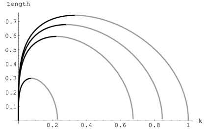
(a)	(b)

Figure 1: (a) The quark antiquark separation $\ell$, in units of $(\pi T_{H})^{-1}$, as a function of $k=\frac{\gamma^{2}}{y_{c}^{4}}$ with $\theta=\left\{0,\frac{\pi}{3},\frac{\pi}{2},\frac{5\pi}{6}\right\}$ from the top to bottom respectively. The dark lines refer to the ”short strings” while the gray lines to the ”long strings”.
(b) The prefactor Z as a function of the angle $\theta$.

To get out of this analysis something which, assuming some kind of universality, should be compared to QCD, we propose to average $Z(\theta)$ over all $\theta$ with a weight $\omega(\theta)$ given by the volume per $\theta$ on $\Omega_{5}$ divided by the total $\Omega_{5}$ volume

$$\omega(\theta)=\frac{vol\Omega_{4}}{vol\Omega_{5}}~{}\sin^{4}\theta~{}=~{}\frac{8}{3\pi}~{}\sin^{4}\theta~{}.$$ (14)

Then the average

$$\overline{Z(\theta)}~{}=~{}\int_{0}^{\pi}Z(\theta)~{}\omega(\theta)~{}d\theta$$ (15)

using (11) can be expressed as an integral over $h$ and evaluated numerically. The result is $\overline{Z}~{}=~{}0.5797$ and gives a suppression factor $\overline{Z}/Z(0)~{}=~{}0.7797$ relative to ref. [7]. We expect a similar averaging to make sense also for the jet quenching parameter.
Comments on the potential
Via AdS/CFT and the standard relation to the Wilson loop the static $q$-$\bar{q}$ potential for large ’t Hooft coupling $\lambda$ is given by

$$V(L,\theta,v)~{}=~{}S_{stat}/T~{},$$ (16)

where $S_{stat}$ is the Nambu-Goto action (4) taken on shell, and one has to identify $\sqrt{\lambda}=R^{2}/\alpha^{\prime}$. Then using (7) one gets

$$V~{}=~{}\frac{T_{H}\sqrt{\lambda}}{\epsilon}~{}\int_{0}^{\ell/2}(y^{4}-\gamma^{2})~{}dx~{}=T_{H}\sqrt{\lambda}~{}\int_{y_{c}}^{\infty}\frac{(y^{4}-\gamma^{2})~{}dy}{\sqrt{(y^{4}-1)(y^{4}-\gamma^{2}-\epsilon^{2}-j^{2}y^{2})}}~{}.$$ (17)

The integral is divergent at $y\rightarrow\infty$. We adopt the usual procedure to subtract two times the action for a string worldsheet located at fixed $x$ and stretching along $y$ from the horizon to infinity. Expressing in addition $\epsilon$ and $\gamma$ via (7),(9) by $h$ and $k$ and transforming the integration variable by $y=y_{c}/w$ we get

$$\frac{V_{ren}}{\lambda^{1/2}T_{H}}=\left\{1+\frac{\gamma^{\frac{1}{2}}}{k^{\frac{1}{4}}}\left(-1+\int_{0}^{1}\Big{(}\frac{1-kw^{4}}{\sqrt{(1-\frac{kw^{4}}{\gamma^{2}})(1-w^{2})(1+hw^{2})}}-1\Big{)}\frac{dw}{w^{2}}\Big{)}\right)\right\}.$$ (18)

As above in the integrals for $\ell$ and $\theta$, the expansion for large $\gamma$ allows a representation in terms of elliptic integrals

$$V_{ren}(L,\theta,v)~{}=~{}T_{H}\lambda^{1/2}\left(1+\frac{\gamma^{1/2}(h+k)}{hk^{1/4}}\Big{(}K(-h)-E(-h)\Big{)}+{\cal O}(\gamma^{-3/2})\right)~{}.$$ (19)

A graphical representation of this leading contribution to the potential as a function of the $q$-$\bar{q}$ separation $\ell$ for various values of the velocity $v$ and the $S^{5}$ angle $\theta$ can be generated by fixing $h(\theta)$ and using (S0.Ex4) and (19) for parametric plots with $k$ as parameter, see fig.2 and fig.3a.

From the field theoretical point of view the potential has to be concave and monotonically growing with $L$. This follows from Osterwalder-Schrader positivity of the Euclidean version of the theory [10]. A generalisation of this rigorous result to the present case, i.e. including the relative $S^{5}$-orientation, has been given in [5]: concavity and monotonic growth in $\ell$ at each fixed $\theta$, $V(L,\theta)\geq V(L,0)$ and, on a more conjectural level, concavity in all directions of the $(L,\theta)$-plane.

Using (S0.Ex4), (19) one gets

$$\left(\frac{\partial V_{ren}}{\partial\ell}\right)_{\theta}~{}=~{}\frac{\gamma\sqrt{h-k}}{2\sqrt{k}}~{},~{}~{}~{}\left(\frac{\partial^{2}V_{ren}}{\partial\ell^{2}}\right)_{\theta}~{}=~{}\frac{h^{2}\gamma^{3/2}}{2(h-3k)k^{3/4}(K(-h)-E(-h))}~{}.$$ (20)

With (10) and $K(-h)-E(-h)<0~{},~{}\forall h\in(0,1]$ we see that, while monotony is always realized, concavity holds on the short string branch ($k<h/3$) only. This perfectly fits with the stability analysis on the string side, where it has been shown that the short (long) string branch is stable (unstable) with respect to small fluctuations [11, 12]. We did not analytically check the extended concavity in the $(L,\theta)$-plane, but the graph in fig.2a suggests its validity.

As seen from fig.2, for large enough $\theta$, part of the short string branch reaches positive values for the potential. Due to our renormalisation prescription this implies a metastable situation [8, 12]. In spite of the stability with respect to small fluctuations, the configuration of two separated worldsheets located at fixed $x$ and stretching along $y$ from the horizon to infinity would be favoured.

At first sight this metastability in the neighbourhood of $\ell_{max}$ could obstruct our averaging proposal for the screening length advocated above. However, another look at fig.3a indicates a weakening of this effect for increasing $\gamma$, such that the critical value for $\theta$ is driven to $\pi$ for $\gamma\rightarrow\infty$, see fig.3b. Since after all our discussion of the screening length concerns its leading behaviour for large $\gamma$, no objection to an averaging over the whole $S^{5}$ remains.

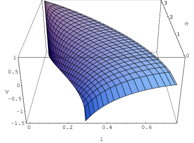
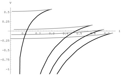
(a)	(b)

Figure 2: (a) Leading order of the potential $V_{ren}$ for the short string branch, in units
  of $\lambda^{\frac{1}{2}}T_{H}$, as a function of separation $\ell$, in units of $\frac{1}{\pi T_{H}}$, and angle $\theta$ for $\gamma=1$.
(b) Leading $V_{ren}$ for $\gamma=1$ and $\theta=\left\{\frac{5\pi}{6},\frac{\pi}{2},\frac{\pi}{3},0\right\}$ from top to bottom respectively.
     The dark lines refer to ”short strings” while the gray lines to ”long strings”.

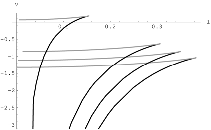
(a)	(b)

Figure 3: (a) Basically the same representation as fig.2b but for $\gamma=cosh(2)$.
(b) Stability analysis represented on the $\gamma$-$\theta$-plane, the short string configuration
     is stable (metastable) up to $\ell_{max}$ in the regions above (below) the curve.

Note that we just discussed the leading large velocity contribution to $V_{ren}$. For the full potential metastability appears even at $\theta=0$ for values of $v<0.45$ i.e. $\gamma<1.12$ [8].
Acknowledgement
This work has been supported in part by the German Science Foundation (DFG) grant DO 447/4-1. H.D. thanks K. Sfetsos for a useful discussion.

References

-
[1]
J. M. Maldacena,
Phys. Rev. Lett. 80 (1998) 4859
[arXiv:hep-th/9803002],
S. J. Rey and J. T. Yee, Eur. Phys. J. C 22 (2001) 379 [arXiv:hep-th/9803001]. - [2] K. Zarembo, Nucl. Phys. B 643 (2002) 157 [arXiv:hep-th/0205160].
-
[3]
N. Drukker,
JHEP 0609 (2006) 004
[arXiv:hep-th/0605151],
N. Drukker, S. Giombi, R. Ricci and D. Trancanelli, “More supersymmetric Wilson loops,” arXiv:0704.2237 [hep-th]. - [4] H. Dorn and H. J. Otto, JHEP 9809 (1998) 021 [arXiv:hep-th/9807093].
- [5] H. Dorn and V. D. Pershin, Phys. Lett. B 461 (1999) 338 [arXiv:hep-th/9906073].
- [6] R. Hernandez, K. Sfetsos and D. Zoakos, JHEP 0603 (2006) 069 [arXiv:hep-th/0510132].
-
[7]
H. Liu, K. Rajagopal and U. A. Wiedemann,
Phys. Rev. Lett. 98 (2007) 182301
[arXiv:hep-ph/0607062].
H. Liu, K. Rajagopal and U. A. Wiedemann, JHEP 0703 (2007) 066 [arXiv:hep-ph/0612168]. - [8] M. Chernicoff, J. A. Garcia and A. Guijosa, JHEP 0609 (2006) 068 [arXiv:hep-th/0607089].
-
[9]
S. D. Avramis and K. Sfetsos,
JHEP 0701 (2007) 065
[arXiv:hep-th/0606190],
S. D. Avramis, K. Sfetsos and D. Zoakos, Phys. Rev. D 75 (2007) 025009 [arXiv:hep-th/0609079],
P. C. Argyres, M. Edalati and J. F. Vazquez-Poritz, JHEP 0704 (2007) 049 [arXiv:hep-th/0612157]. - [10] C. Bachas, Phys. Rev. D 33 (1986) 2723.
- [11] J. J. Friess, S. S. Gubser, G. Michalogiorgakis and S. S. Pufu, JHEP 0704 (2007) 079 [arXiv:hep-th/0609137].
- [12] S. D. Avramis, K. Sfetsos and K. Siampos, Nucl. Phys. B 769 (2007) 44 [arXiv:hep-th/0612139].