Non-parametric inversion of gravitational lensing systems with few images using a multi-objective genetic algorithm

Abstract

Galaxies acting as gravitational lenses are surrounded by, at most, a handful of images. This apparent paucity of information forces one to make the best possible use of what information is available to invert the lens system. In this paper, we explore the use of a genetic algorithm to invert in a non-parametric way strong lensing systems containing only a small number of images. Perhaps the most important conclusion of this paper is that it is possible to infer the mass distribution of such gravitational lens systems using a non-parametric technique. We show that including information about the null space (i.e. the region where no images are found) is prerequisite to avoid the prediction of a large number of spurious images, and to reliably reconstruct the lens mass density. While the total mass of the lens is usually constrained within a few percent, the fidelity of the reconstruction of the lens mass distribution depends on the number and position of the images. The technique employed to include null space information can be extended in a straightforward way to add additional constraints, such as weak lensing data or time delay information.

1 Introduction

The deflection of light from a distant source by the gravitational influence of an intermediate object gives rise to so-called gravitational lensing systems. Images of a source not only provide information about said source, but also encode properties about the mass of the object responsible for the deflection: the gravitational lens.

Gravitational lens inversion, i.e. the determination of the mass density of the lens based on observed image properties, is the focus of this article. Lens inversion procedures are often divided into two categories: parametric and non-parametric methods. Parametric techniques approximate the mass distribution of the lens by a function that is characterized by a small number of parameters. They then optimize these parameters to provide the best possible fit to the observed data. Several such algorithms have been proposed (e.g. lensclean (Kochanek & Narayan, 1992)), and several software packages are publicly available (e.g. gravlens (Keeton, 2001) and lenstool (Kneib et al., 1993)). Non-parametric inversion methods try to avoid this restriction, for example by pixellizing the mass distribution (e.g. Saha & Williams (1997)), pixellizing the lens potential (e.g. Bradač et al. (2005), Koopmans (2005)) or by dynamically adjusting the number of basis functions used (e.g. Diego et al. (2005)).

In a previous article (Liesenborgs et al., 2006), we described a non-parametric inversion routine, intended for strong lensing systems containing many multiply imaged sources. Using a genetic algorithm, we showed through simulations that the mass density of the lens can be reliably retrieved and that the reconstructed sources closely resemble their original counterparts. While such data is currently available (Broadhurst et al., 2005) and more of these systems are likely to be discovered in the future, they are currently far outnumbered by systems containing a handful of images of only one or a few sources.

For this reason, we felt the need to investigate the performance of the original procedure and the required modifications when confronted with a few-sources situation. As in the previous work, simulations are used to determine what can be inferred about the mass density when all the necessary information is available with great accuracy, thereby placing fundamental limits on the amount of information which can be extracted from such a lensing scenario. Again, we will try to avoid imposing any prior on the mass density of the lens: only the information contained in the observed images is used.

The situation being studied here, bears resemblance to the work of Abdelsalam et al. (1998): there, based on the image locations of a few sources, a pixellized mass distribution of a cluster lens was reconstructed. However, while their algorithm uses one position per image, the method presented here makes use of the complete images. Another important difference is that the method described in that article searches for the mass distribution which follows the light map as closely as possible. Below, no information about the light map of the gravitational lens will be used.

The following section contains a brief review of the lensing formalism, genetic algorithms and the original inversion technique. Section 3 illustrates the difficulties encountered with the procedure and describes which measures can be taken to overcome them. After illustrating the effect of these modifications in sections 4 and 5, our conclusions are summarized in section 6.

2 Review

2.1 Lensing formalism

To first post-Newtonian order, the gravitational lens effect can be well described by the so-called lens equation, describing a mapping $\mbox{\boldmath$\beta$}(\mbox{\boldmath$\theta$})$ from the image plane onto the source plane. Our focus is on the strong lensing effect, in which multiple images of a source are generated. It is important to note that when these images are projected back onto the source plane using the lens equation, they must coincide since they are images of the same source. A thorough review of the gravitational lensing formalism can be found in Schneider et al. (1992).

2.2 Genetic algorithms

Genetic algorithms implement a problem-solving strategy based on the principle of natural selection, present in biological systems. The procedure starts with a ‘population’ of trial solutions, stored in an encoded form which is often referred to as the genome. Each member of the population is then evaluated and a fitness measure is assigned. Using the current population, a new one is created by combining genomes – mimicking sexual reproduction – or by copying them – mimicking asexual reproduction. When selecting genomes in this process, a key ingredient of the genetic algorithm is to apply some form of selection pressure: genomes which are deemed more fit, should have a higher probability of creating offspring. This can be achieved by ranking the genomes according to their fitness measures and by assigning a higher selection probability to the genomes with a more favorable rank. After introducing some random mutations to ensure genetic diversity, the newly created population replaces the old one and the procedure is repeated until a stopping criterion is fulfilled. In some cases one can choose to apply ‘elitism’ and copy the best genome in a generation directly to the next generation.

Research into this kind of evolutionary optimization was pioneered by Holland (1975) and the type of genetic algorithm introduced there is now referred to as the canonical genetic algorithm. Currently, genetic algorithms are available in many forms and are used to solve a wide variety of (often high-dimensional) problems, including the automatic generation of computer algorithms (e.g. Koza (1992)). For an excellent introduction to the use of genetic algorithms in an astrophysical context, the interested reader is referred to Charbonneau (1995).

2.3 Inversion method

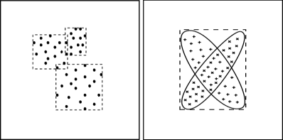
Figure 1: Left panel: back-projected images are enclosed by rectangles of which the sides are parallel to the coordinate axes. The genetic algorithm produces mass distributions which cause these rectangles to overlap increasingly well. Right panel: when different images of an elliptical source are projected back onto the source plane, the situation shown has a good fitness value, even though the images do not overlap well. This problem is easily resolved by allowing the enclosing rectangles to be rotated.

The inversion procedure requires the user to define a square region in which the strong lensing mass will be reconstructed. This region is subdivided in a uniform grid of cells. Each of the grid cells is assigned a basis function, more specifically a projected Plummer sphere (Plummer, 1911). Writing the mass density distribution of the gravitational lens as a weighted sum of these basis functions, the gravitational lens effect is described by the following lens equation:

$$\mbox{\boldmath$\beta$}(\mbox{\boldmath$\theta$})=\mbox{\boldmath$\theta$}-\frac{D_{ds}}{D_{s}D_{d}}\frac{4G}{c^{2}}\sum_{i=1}^{N}\frac{\mbox{\boldmath$\theta$}-\mbox{\boldmath$\theta$}_{s,i}}{|\mbox{\boldmath$\theta$}-\mbox{\boldmath$\theta$}_{s,i}|^{2}+\theta_{P,i}^{2}}M_{i}\mathrm{.}$$ (1)

Here, $\mbox{\boldmath$\theta$}_{s,i}$ is the center of a basis function, $M_{i}$ is its total mass and $\theta_{P,i}$ a measure of its width. A genetic algorithm is then applied to determine the weights $M_{i}$ of each basis function and the resulting mass distribution is used to create a new grid, in which regions containing a larger fraction of the mass will be subdivided further. A Plummer basis function is assigned to each new grid cell and the genetic algorithm again determines the appropriate weights. This procedure can be repeated a number of times, depending on the desired level of detail.

The genetic algorithm is clearly at the heart of this inversion method. For details about genome encoding, reproduction and mutation, the reader is referred to Liesenborgs et al. (2006). Here, we will focus on the fitness evaluation since this determines the evolution of the algorithm towards a solution. The input of the entire procedure consists of the images associated with each source. Using the Plummer weights $M_{i}$ stored in a genome, equation (1) is used to project these images back onto their source planes. As was stated earlier, the correct lens equation generates overlapping images for each source, and it is precisely this criterion that is applied to determine the fitness of a genome. The left panel of Fig. 1 illustrates how the degree of overlap is measured. Each back-projected image is surrounded by a rectangle of which the sides are parallel to the coordinate axes. If the back-projected images of a source overlap perfectly, so will the rectangles that surround each image. For this reason, the degree to which the images overlap will be approximated by the overlap of the associated rectangles. This can easily be calculated: two rectangles will coincide if their corners coincide, which suggests that the separation between corresponding corners can be used to measure the amount of overlap. To assign a fitness value, corresponding corners of the rectangles are connected with imaginary springs and the potential energy of the situation is calculated. Note that in calculating distances between corners, the average size of the rectangles is used as the length scale. This makes sure that the overlap is measured relative to the size of the source. The same procedure is repeated for the other sources and the sum of all these potential energies is used as the fitness measure of the genome. Lower values indicate a better overlap of the back-projected images and therefore correspond to genomes which are deemed more fit. Several runs of this inversion routine typically generate solutions which differ somewhat. This is a result of the inherent randomness present in genetic algorithms which will manifest itself especially when the grid is refined further. Averaging a number of individual solutions yields a final mass density which is far more smooth than any individual solution and inspecting the standard deviation provides information about the amount of disagreement between the generated solutions. This way, the standard deviation of individual solutions yields an indication of the uncertainty in the reconstructed mass density. Note that this is only an indication, as it does not include systematic effects.

Tests with simulations indicate that when many multiply imaged sources are available, this procedure not only creates an excellent map of the lensing mass, but also retrieves the sizes and positions of the sources remarkably well. No prior assumptions are made regarding the mass density or the sources, and by construction, no negative mass densities will arise. The radial images are used in an effective way, i.e. the relative weight of a given image in the fitness value does not depend on its surface area, as in image fitting methods. This is an important feature if one is interested in obtaining the best possible estimate of the central mass density of the lens.

Like other non-parametric inversion algorithms, in reality there are simply a very large number of parameters: the weights of a large amount of basis functions. Plummer basis functions were chosen mainly for simplicity, but also because earlier tests indicated that a wide variety of mass distributions can be approximated by a sum of Plummer basis functions. Similar inversion results can be obtained using Gaussian basis functions; square basis functions appear to be less suitable as they quickly cause complex caustic structures.

3 A first test and algorithm extensions

The inversion technique described above is intended to be used when many multiply imaged sources are available to constrain the mass distribution of the lens. To illustrate the problems one encounters in a situation where the lensing mass is poorly sampled, we use the sources and the lens mass density shown in Fig. 2. The sources have an elliptical shape and are positioned at $z=2.5$ and $z=1.5$ respectively; the lensing mass is located at $z=0.45$. In this article, we use a standard CDM cosmology with a matter density $\Omega=1$ and a Hubble parameter $H_{0}=70$ km s^-1 Mpc^-1 for simplicity. As can be derived from the caustic structures, each source produces five images, the positions of which are displayed in the left panel of Fig. 3. The critical lines corresponding to both redshifts are also indicated in this figure.

3.1 Difficulties

When the procedure outlined above is applied to the images of Fig. 3 (left panel), some undesired effects can be observed. The first one is demonstrated in the right panel of Fig. 1. Because the rectangles used to determine the degree of overlap in the back-projected images are aligned with the coordinate axes, crossing elliptical shapes will be interpreted as overlapping images. Due to the large number of multiply imaged sources in the original study, and hence the large number of independent constraints, this problem did not manifest itself before. The solution to the problem is clear: the rectangles which are placed around the back-projected images should be rotated until they are aligned with their respective images. This can be done in an efficient way using the ‘rotating calipers’ algorithm (Shamos, 1979).

Another problem that surfaced due to the limited number of constraints, is non-overlapping brightness distributions of back-projected images. However, the fitness measure can easily be modified to correct this behavior: each rectangle is placed at a height corresponding to the maximal brightness value of the corresponding image. The average height is used as length scale in this direction and the fitness value is calculated as before, now using three-dimensional virtual springs instead of two-dimensional ones. The situation is illustrated in Fig. 4. More elaborate schemes can easily be implemented to ensure a suitable overlap of the back-projected images, at the cost of increasing the computer work load, but this will suffice for our goals. When these extensions are added to the original genetic algorithm, it is able to create solutions which produce overlapping images when projected back onto the source plane, both in the position and brightness domains.

Unfortunately, when comparing the images predicted by the best lens solution with the observed ones, a more serious problem presented itself. Because of the non-parametric nature of the reconstruction and the lack of firm constraints, the reconstructed lens mass distribution can contain many small-scale fluctuations that generate a host of images other than the observed ones. The right panel of Fig. 3 illustrates this undesired behavior.

Figure 2: Left panel: mass distribution of the input lens (placed at redshift $0.45$) used in the first simulation. The value of $\Sigma_{cr}$ was evaluated at redshift $2.5$. Middle panel and right panel: the two sources, placed at redshifts $2.5$ and $1.5$ respectively, used in the first simulation, together with the caustic structures at these redshifts.

Figure 3: Left panel: the lens and sources of Fig. 2 cause ten images to be generated. The critical lines of the first source are shown as solid lines, those of the second source as dashed lines. The images of the second source are enclosed by small squares. Right panel: the original algorithm can easily produce solutions which cause the back-projected images to overlap well. However, the reconstructed sources and lens in general cause many undesired images to be produced, as is illustrated in this figure.

Figure 4: Back-projected images are surrounded by rotated rectangles and placed at a height corresponding to the maximal brightness values of the images. Corresponding corners are connected with virtual springs (indicated by thick dotted lines) and the potential energy of the situation is used as the fitness measure. This way, reconstructed sources will also overlap in the brightness domain.

3.2 Using the null space

One possible solution to avoid this multitude of spurious images, is to impose some kind of prior on the lensing mass. For example, one could modify the fitness criterion to favor smoother mass distributions. Undoubtedly, this would reduce the number of extra images since smoother mass distributions have less complex caustic structures. However, this goes against the spirit of our endeavor, which is to find out how much information can be retrieved non-parametrically from a few-image lens system.

In order to avoid introducing this kind of bias in the generated solutions, a different approach is used. Note that there is still much information available that has not yet been used. Points in the image plane which are not part of an image of the source, i.e. the null space, provide additional constraints: if they are projected back onto the source plane using the correct lens equation, none of these points will lie inside the source area. Otherwise, an image would be visible at that specific location. Using the null space was already suggested in Diego et al. (2005), but there, only null space points adjacent to the images were used. This can avoid the acceptance of solutions that produce images larger than the observed ones, but it obviously fails to avoid the extra images.

To incorporate the information in the null space, two schemes have been explored. In the first one, a regular grid of null space points is generated and the points which fall inside an input image are removed. To avoid generating images which lie relatively far from the other images, and thereby generating more mass than is necessary, the area in which the null space points are generated should be chosen large enough, i.e. somewhat larger than the area of the images themselves. An appropriate size can easily be discovered after a few attempts, but 10-20% larger is usually adequate. After projecting the images back onto the source plane, their envelope is calculated. This is the smallest convex polygon enclosing all the back-projected points, and is used as the current estimate of the source shape. Next, each point in the null space is projected back onto the source plane and the number of points which lie inside the reconstructed source are counted. Clearly, one would like this count to be as low as possible, since our objective is to remove the extra images. Note that by only considering a discrete number of points in the null space, it is possible that small images are generated which lie in between null space points.

Instead of simply using points, one can also divide the null space into a number of small triangles, similar to the approach in Blandford & Kochanek (1987). When these are projected back onto the source plane, for each triangle the amount of overlap with the reconstructed source is calculated. The corresponding area of the triangle in the image plane is then used as this triangle’s contribution to the null space fitness measure. Again, this number should be as low as possible to avoid generating extra images. The advantage of this method is that it becomes easier to avoid small undesired images, at the cost of increased computational complexity.

In any case, at this point two numbers describe the fitness of a genome under study: one describes the overlap of the back-projected images, the other takes the null space into account. At first, one might try summing the two fitness values, multiplying each term with a specific weight. Indeed, our first successful lens reconstructions used such a technique. However, using a weighted scheme requires the end-user to find and specify acceptable weight values. Furthermore, using specific weight values will automatically bias the path followed in the search space as the optimization routine progresses.

3.3 A multi-objective genetic algorithm

Fortunately, there is no need to specify a weight factor. Genetic algorithms are excellent solvers of multi-objective or multi-criterion optimization problems. Below, some key concepts are introduced. The interested reader is referred to Deb (2001) for an in-depth treatment of this subject.

In a multi-objective genetic algorithm a genome has several fitness measures, each one related to a specific aspect of the optimization problem. A genome is said to dominate another genome if two criteria are met: (i) it is not worse in all fitness measures, and (ii) it is strictly better in at least one fitness measure. Using this concept of dominance, one can identify in a population the members which are not dominated by any other genome, resulting in the so-called non-dominated set. The concept of a non-dominated set is used to devise a new ranking scheme, as there is no longer a single fitness criterion to base the ranking procedure on. First, the non-dominated set of the entire population is calculated. The genomes in this set will receive the highest rank. After removing this set from the population, a new non-dominated set is identified and these genomes receive the next-to-highest rank. The procedure is repeated until all genomes of the population are processed. Afterwards, the genetic algorithm can proceed as before.

When there are conflicting objectives, there is a whole range of optimal solutions: the Pareto-optimal front. There exist procedures to preserve a certain amount of diversity in the population, allowing the Pareto-optimal front to be well sampled by the genetic algorithm. In our specific case however, the objectives are not conflicting and no further modifications are required.

Figure 5: Left panel: when the null space is taken into account, this mass distribution was obtained after averaging twenty individual solutions. Comparing this to the left panel of Fig. 2 shows that much of the general appearance is retrieved. Middle panel and right panel: the reconstructed sources lie close to the true source positions (indicated by crosses). When these figures are compared to the middle and right panels of Fig. 2, it is clear that much of the same caustic structure is present in the reconstruction.

4 Simulation results

Figure 6: Left panel: the difference between the true mass density and the average solution, relative to the critical mass density for a source at redshift $2.5$. This clearly shows that the true shape of the mass density peaks cannot be determined accurately. Right panel: standard deviation of the twenty individual reconstructed mass densities. Individual solutions clearly disagree about the exact shape of the mass density around the peak positions.

Figure 7: Left panel: the reconstructed source and lens of Fig. 5 generated these images and critical lines. The correspondence with the left panel of Fig. 3 is striking. Right panel: the circularly averaged mass densities of input lens and reconstruction, as seen from the mass density peak at $(0.5,-0.5)$.

Figure 8: Left panel: total mass within a specific radius for both input lens and reconstruction, as seen from the origin. Clearly, the total mass is estimated well within a radius of 1′. Right panel: the amount of disagreement in total mass within a specific distance from the origin. Again, within a radius of 1′ the agreement is very good.

Using the procedure outlined above, it is now straightforward to generate solutions which indeed only produce the input images. Averaging twenty such solutions yields the mass density and reconstructed sources shown in Fig. 5. Comparing this figure with Fig. 2, one immediately notices the striking resemblance. This proves that our method is capable of reproducing, at least qualitatively, the mass density distribution of a gravitational lens based on the positions, redshifts, and shapes of very few images and on null space information. The peaks in the reconstructed mass density appear to be somewhat stronger than those of the input lens. The reconstructed sources are very similar in shape to the true sources and their positions lie very close to those of the input sources. The reconstructed sources are, however, more extended than the input sources. The caustic structure presented in the middle and right panels of Fig. 5 are strikingly similar to but more extended than those of the input lens, presented in the middle and right panels of Fig. 2. In this example the method using null space triangles was used, based on a regular $64\times 64$ grid, covering an area of $3.3\times 3.3$ arcmin².

It is interesting to take a look at the difference in mass densities between original and reconstructed lens. The left panel of Fig. 6 shows that the mass density around the peak positions is not reconstructed very well. Inspecting the right panel of the same figure, which displays the standard deviation of the individual solutions, it is clear that precisely these regions differ strongly among the solutions. When the reconstructed source and lens are used to reproduce the images, the result shown in the left panel of Fig. 7 is obtained. The ten input images are indeed reproduced and the critical lines closely resemble those of Fig. 3 (left panel). One cannot ask more from any lens inversion algorithm. The right panel of Fig. 7 shows the circularly averaged mass density, centered on the mass density peak at $(0.5,-0.5)$. This plot visualizes once more the overestimated mass density in that region, although the same general features are clearly present in both original and reconstructed profile. When the total mass of the lens is calculated, the agreement is excellent within a radius of 1′, differing by only a few percent from the true mass, as is shown in Fig. 8. Beyond that radius, the difference starts to increase, indicating that using only the strong lens effect, one cannot obtain a firm handle on the mass density outside the radius of the outer images.

It was mentioned before that the reconstructed sources are somewhat larger (and brighter) than the true sources. Since two sources are used in this simulation, this cannot be the result of the mass sheet degeneracy (e.g. Saha (2000)) and some other type of degeneracy must be at work here. In a single-source scenario, the mass-sheet degeneracy is artificially broken: the mass density of the reconstructions quickly drops to zero outside of the grid and it is unlikely that the procedure will construct a circular area of constant density using (randomly initialized) basis functions arranged on a grid.

5 A second test

One might argue that a system with two sources and ten images still provides a relatively large number of constraints. For this reason, let us now turn to a simple five-image system, created by an elliptical mass distribution. The source and its corresponding images are depicted in the left panel of Fig. 9. The redshifts of the source and the lens are $2.5$ and $0.45$ respectively. Note that in this situation the mass-sheet degeneracy is artificially broken, as explained above.

Figure 9: Left panel: the source used in the simulation of a gravitational lens system with an elliptical mass distribution, relative to the caustic structure. This situation creates five images, which are used as the input of the inversion routine. Center panel: the reconstructed source, relative to the predicted caustics when using a moderately subdivided grid and averaging ten individual solutions. Note that the source and the caustic structure are more extended than their original counterparts. Shown below are the five resulting images as well as the critical lines. Right panel: similar to the center panel, but using a finely subdivided grid. The fitness measures did not improve considerably compared to the situation in the center panel.

In this case, the inversion algorithm seems to easily produce solutions causing a critical line to intersect the two rightmost images. To avoid this, the brightness overlap and positional overlap were used as two separate fitness measures. Since their combination can be seen as a weighting scheme, decoupling them allows a broader search in the model space. Afterwards, the genetic algorithm was indeed able to consistently find solutions which reproduce the input images. After averaging ten solutions obtained using a moderately subdivided grid, the results shown in the center panel of Fig. 9 were obtained. This clearly resembles the true situation, although the source is again larger and brighter. If the grid is subdivided further, this results in the situation depicted in the right panel of Fig. 9, showing more complex critical lines and corresponding caustic structure.

It is important to note that the resulting genome fitness did not improve significantly by using a finer grid. In practice, due to a lack of constraints, one may simply opt for the least complex reconstruction. However, as is shown in the right panel of Fig. 9, the algorithm is indeed able to produce viable solutions containing small-scale variability introduced by using approximately one thousand basis functions. This ability to handle different scales well is, of course, required to qualify as a truly non-parametric technique.

6 Discussion and conclusion

In this article we have presented an extension of our previously proposed inversion algorithm, which was intended to be used on a strong lensing system with many multiply imaged sources. Since currently the number of known strong lensing systems with few sources far exceed those with many, we felt it was appropriate to study the necessary extensions of the original procedure to allow such systems to be inverted non-parametrically. The modifications presented above still use only physically motivated arguments and do not impose any prior on the reconstructed mass density. The inclusion of the null space led to an additional fitness measure, which can be handled efficiently and without the need of a weight parameter using a multi-objective genetic algorithm. In a similar way one could incorporate even more constraints, e.g. from the weak lensing regime or from time delay measurements, without the need for weights. This generic way of handling various types of constraints is clearly a great advantage of the proposed inversion method.

We found that including brightness information is in this case necessary to ascertain acceptable source reconstructions. It is interesting to note that even without this extra information, the inclusion of the null space already brings out most of the general structure of the mass distribution. This suggests that uncertainty in measured image intensities will not prevent a good reconstruction of the mass density, which is important from a practical point of view.

Although the examples shown above seem to suggest a bias towards larger and brighter reconstructed sources, it is easy to create a scenario in which the genetic algorithm will cause the reconstructed sources to be smaller and dimmer. This kind of degeneracy can only be resolved if more data are available or some prior is imposed on the source. The fact that the true source features cannot be obtained with certainty even when all the information is available with the greatest accuracy, indicates that care should be taken when interpreting source data obtained by strong lens inversion in general.

Deviations from the true mass density are to be expected, not only because of the sparse sampling of the lens equation, but also because of the inherent degenerate nature of the lens inversion problem. Nevertheless, the similarities between the original lens systems and the reconstructions are remarkable, especially when taking into consideration that no prior information about the lens was needed. This indicates that much information is present in a strong lensing system and that it can be extracted non-parametrically using only information about the observed images.

Above, we have investigated only the ideal situation, when all image positions and fluxes are known accurately. Practical difficulties like incomplete null space information, obscured images, measurement errors or the effect of a point spread function will further reduce the information content of a strong lensing system. The precise impact of these factors will require further research. Furthermore, if relatively large images are present, it is likely that the simple technique to determine the overlap between images will fail. We are currently exploring methods to take image substructure into account to be able to handle such cases effectively.

References

- Abdelsalam et al. (1998) Abdelsalam H. M., Saha P., Williams L. L. R., 1998, MNRAS, 294, 734
- Blandford & Kochanek (1987) Blandford R. D., Kochanek C. S., 1987, ApJ, 321, 658
- Bradač et al. (2005) Bradač M., Schneider P., Lombardi M., Erben T., 2005, A&A, 437, 39
- Broadhurst et al. (2005) Broadhurst T., Benítez N., Coe D., Sharon K., Zekser K., White R., Ford H., Bouwens R., Blakeslee J.,et al., 2005, ApJ, 621, 53
- Charbonneau (1995) Charbonneau P., 1995, ApJS, 101, 309
- Deb (2001) Deb K., 2001, Multi-Objective Optimization Using Evolutionary Algorithms. John Wiley & Sons, Inc., New York, NY, USA
- Diego et al. (2005) Diego J. M., Protopapas P., Sandvik H. B., Tegmark M., 2005, MNRAS, 360, 477
- Holland (1975) Holland J. H., 1975, Adaptation in natural and artificial systems. University of Michigan Press, Ann Arbor
- Keeton (2001) Keeton C. R., 2001, ArXiv Astrophysics e-prints
- Kneib et al. (1993) Kneib J. P., Mellier Y., Fort B., Mathez G., 1993, A&A, 273, 367
- Kochanek & Narayan (1992) Kochanek C. S., Narayan R., 1992, ApJ, 401, 461
- Koopmans (2005) Koopmans L. V. E., 2005, MNRAS, 363, 1136
- Koza (1992) Koza J. R., 1992, Genetic Programming: On the Programming of Computers by Means of Natural Selection (Complex Adaptive Systems). The MIT Press
- Liesenborgs et al. (2006) Liesenborgs J., De Rijcke S., Dejonghe H., 2006, MNRAS, 367, 1209
- Plummer (1911) Plummer H. C., 1911, MNRAS, 71, 460
- Saha (2000) Saha P., 2000, AJ, 120, 1654
- Saha & Williams (1997) Saha P., Williams L. L. R., 1997, MNRAS, 292, 148
- Schneider et al. (1992) Schneider P., Ehlers J., Falco E. E., 1992, Gravitational Lenses. Gravitational Lenses, XIV, 560 pp. 112 figs.. Springer-Verlag Berlin Heidelberg New York. Also Astronomy and Astrophysics Library
- Shamos (1979) Shamos M. I., 1979, PhD thesis, Yale University