A Combined Spitzer and Chandra Survey of Young Stellar Objects in the Serpens Cloud Core.
Abstract
We present Spitzer and Chandra observations of the nearby (260 pc) embedded stellar cluster in the Serpens Cloud Core. We observed, using Spitzer’s IRAC and MIPS instruments, in six wavelength bands from 3 to 70 , to detect thermal emission from circumstellar disks and protostellar envelopes, and to classify stars using color-color diagrams and spectral energy distributions (SEDs). These data are combined with Chandra observations to examine the effects of circumstellar disks on stellar X-ray properties. Young diskless stars were also identified from their increased X-ray emission.
We have identified 138 YSOs in Serpens: 22 class 0/I, 16 flat spectrum, 62 class II, 17 transition disk, and 21 class III stars; 60 of which exhibit X-ray emission. Our primary results are the following: 1.) ten protostars detected previously in the sub-millimeter are detected at m, seven at m, 2.) the protostars are more closely grouped than more evolved YSOs (median separation : pc), and 3.) the luminosity and temperature of the X-ray emitting plasma around these YSOs does not show any significant dependence on evolutionary class. We combine the infrared derived values of and X-ray values of for 8 class III objects and find that the column density of hydrogen gas per mag of extinctions is less than half the standard interstellar value, for . This may be the result of grain growth through coagulation and/or the accretion of volatiles in the Serpens cloud core.
1 Introduction
Surveys of molecular clouds indicate that 60% of young stars form in clusters (Carpenter, 2000; Allen et al., 2006; Megeath et al., in prep). It is therefore important to study star formation in clusters to understand the influence of the cluster environment in the process of star and planet formation. Of fundamental importance is the understanding of the spatial structure of clusters, and of the evolution of that structure. Observations with the Spitzer and Chandra Space Telescopes are of great importance in the study of cluster structure as they provide the means to identify young stellar objects from the protostellar to pre-main sequence phases, and to categorize these objects into the canonical evolutionary classes (class 0/I, II and III (Lada & Wilking, 1984)). The number and distribution of sources in each of these classes provides unique information on the distribution of star formation sites, the motion of the stars after they form, and the dynamical state of the cluster at large. From these studies, we can better understand the physical processes that govern the fragmentation of molecular clouds, the ensuing trajectories that the resulting young stars make through the cluster, and the eventual fate of the embedded cluster. Clusters also serve as laboratories for the evolution of young stellar objects, and can be used to study the evolution of disks around young stars and the evolution of hot X-ray emitting plasma commonly found around such stars (see for example: Gutermuth et al. (2005); Haisch et al. (2001); Preibisch & Feigelson (2005); Hernadez et al. (2006))
In this paper, we describe a detailed study of the population of young stellar objects in the Serpens cluster identified by observations with Spitzer and Chandra. The Serpens region is an example of a very young, deeply embedded cluster, containing a number of protostars (Harvey et al., 2006; Hurt & Barsony, 1996; Eiroa et al., 1992, 2005; Kaas et al., 2004; Testi et al., 2000). The embedded cluster is heavily extinguished, with a peak extinction exceeding 40 magnitudes in the visual. At a distance of 260 pc, the Serpens cloud core is one of the nearest regions of clustered star-formation to the Sun (see Straiz̆ys et al. (2003) for a discussion of the distance to Serpens). This makes it an excellent candidate for study with Spitzer as it is close enough to both resolve the individual members and to detect the lowest mass members to below the hydrogen-burning limit. Furthermore, the Serpens cluster is rich in protostars. Sub-millimetre and millimetre observations of the region, at 450 , 850 and 3 mm, identify at least 14 objects in the Serpens Cloud Core (Testi et al., 1998, 2000; Davis et al., 1999; Hogerheijde et al., 1999; Harvey et al., 2006). In this paper, we extend the sample of known young stellar objects in Serpens using the high sensitivity of Spitzer and Chandra. We then discuss three topics: the mid-IR spectral energy distributions of protostellar objects detected in the sub-millimeter, the spatial distribution of the Serpens cluster members, and finally, the X-ray properties of the young stellar objects as a function of their evolutionary class.
2 IRAC & MIPS Data Reduction
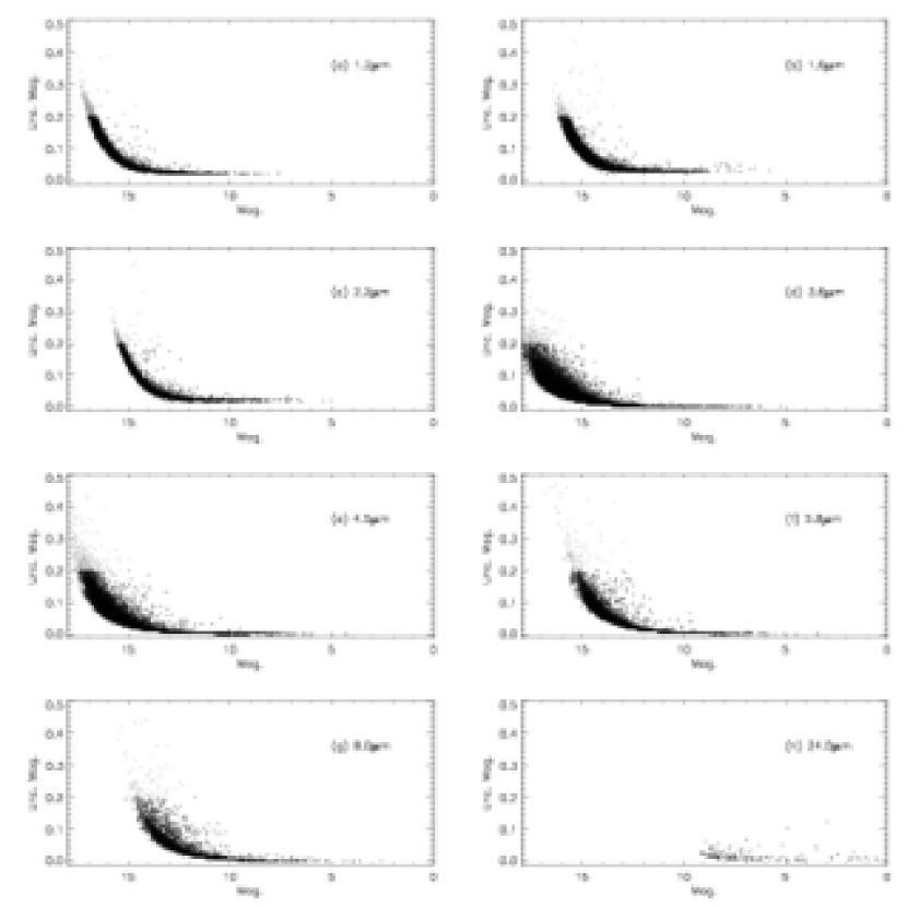
We have obtained Spitzer images of the Serpens Cloud Core in six wavelength bands: the 3.6, 4.5, 5.8 and 8.0 m bands of the InfraRed Array Camera (IRAC; Fazio et al. (2004)) and the 24 m and 70 m bands of the Multi-band Imaging Photometer for Spitzer (MIPS; Rieke et al. (2004)). The photometry extracted from these data was supplemented by , and -band photometry from the 2MASS point source catalog (Skrutskie et al., 2006), resulting in data in nine photometric bands spanning 1-70 m. The uncertainties for the point sources as a function of magnitude are shown in Fig. 1. In the following analysis, only data with uncertainties magnitudes were used. Below, we describe the observations, image reduction and photometry for the Spitzer data.
2.1 IRAC:
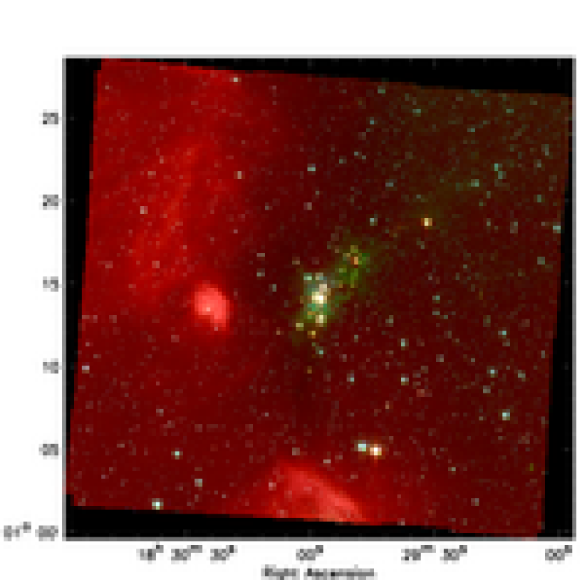
The Spitzer Space Telescope has observed the Serpens cluster with the IRAC instrument at two different epochs. The first epoch was on 1st April 2004; these observations were part of the Guaranteed Time Observation program PID 6, The Structure and Incidence of Embedded Clusters. The second epoch was on 5th April 2004, during which Spitzer executed observations from PID 174 from the cores to disks (c2d) legacy program. The mosaicked regions cover a field in all four of the IRAC wavelength bands (Fig.2). The field is centered on the main Serpens cluster in the Northern Cloud Core. The observations were taken in the high dynamic range mode with a 12 second frame time. In each epoch, two dithered 10.4 second frames and two dithered 0.4 second frames were obtained at each map position.
The analysis used the basic calibrated data (BCD) FITS images from the S11.4 pipeline of the Spitzer Science Center. These data were combined into mosaics using the MOPEX program. The 3.6 m and 4.5 m images were pre-processed by using the IDL-based pulldown corrector by Lexi Moustakas 111http://ssc.spitzer.caltech.edu/irac/pulldown/, and then additional interactive processing steps were applied to locate and remove the remaining column pulldown and mux bleed artifacts in the 3.6 m and 4.5 m images, and banding effects in the 5.8 m and 8.0 m images (Hora et al., 2004). The overlap correction module was used to minimize instrumental offsets between adjacent frames, and the mosaics were constructed on a pixel scale of 0.8627 ′′/pixel, or the IRAC pixel size. The typical total integration time is 41.6 seconds per pixel, although in some regions near the edges of the mosaic, the integration time is 20.8 seconds. The calibration uncertainty across the IRAC bands is estimated at mag (Reach et al., 2005). In addition, there are 5% position dependent variations in the calibration of point sources in the flat-fielded BCD data; these have not been corrected for in our data. Furthermore, these systematic uncertainties have not been added into the random photometric uncertainties reported in this paper.
We used a custom IDL program for point source finding; this program was a heavily modified version of the DAOfind program in the IDLPHOT package (Landsman, 1989). This program first creates a smoothed version of the mosaic by convolving with a Gaussian with pixels, approximately double the FWHM of the point sources, and then subtracts the smoothed version from the mosaic to filter out the extended nebulosity. The noise in a pixel region around the source was calculated to assess the combined instrumental noise, shot noise and noise from the spatially varying extended nebulosity. Point sources with peak values more than 5 above the background were considered candidate detections. After the point sources were identified, aperture photometry then was obtained using the aper.pro program in the IDLphot package. An aperture radius of 2.8 pixels () was used, and a sky annulus from 4.2 to 8.4 pixels ( to ) was used to measure the contribution from extended emission in the aperture. The zero points for these apertures were, 17.8204, 17.3025, 16.7408, and 15.9440 mag for the 3.6, 4.5, 5.8, and 8.0 m bands, respectively, in the native BCD image units of MJy pixels sr-1.
There were 25853, 22703, 6595, and 3946 detections in the 3.6, 4.5, 5.8, and 8.0 respectively, with uncertainties less than 0.2 mag, with 2758 of these detected in all four IRAC bands. The sensitivity of the 8.0 band is the limiting factor in four band detections: it suffers from lower photospheric fluxes, higher background emission, and the presence of bright, structured nebulosity in some parts of the image. The detection threshold in the 3.6 band was 17 magnitudes - far below the hydrogen burning limit for a 1 Myr old star at the distance of Serpens (12 mag at 3.6 m (Baraffe, 1998)).
2.2 MIPS:
Spitzer observed the Serpens cluster twice with the Multiband Imaging Photometer for Spitzer (MIPS; Rieke et al. 2004). In both epochs, the medium scan rate was used. For the first epoch, part of the Guaranteed Time Observation program PID 6, taken on the 6th April 2004, six 0.5 degree scan legs with full-array cross-scan offsets were used. For the second epoch observations (PID 174), 12th April 2005, 12 scan legs of length 0.5 degrees and half-array cross-scan offsets were used. In both epochs, the total map size was approximately 0.5 x 1.5 degrees including the overscan region. All three MIPS bands are taken simultaneously in this mode; because the data at 160 micron are saturated, we do not consider it in our subsequent analysis. The 2nd epoch map had full 70 m coverage, while the first epoch mapped only six wide bands, covering half of the map. Both epochs were combined to form the final maps. The typical effective exposure time per pixel is about 80 seconds at 24 m and 40 seconds at 70 m. The MIPS images were processed using the MIPS instrument team Data Analysis Tool, which calibrates the data and applies a distortion correction to each individual exposure before combining into a final mosaic (Gordon et al., 2005). The data were further processed using various median filters to remove saturation effects and column-dependent background structure. The resulting mosaics have a pixel size of at 24 m and at 70 m.
Stars in the 24 m mosaic were then identified using PhotVis (Gutermuth, 2005), which searched for all point sources with peaks 5 times the RMS noise. Aperture photometry in a 5 pixel aperture was performed on these sources with PhotVis and the photometry was corrected to a 12 pixel aperture radius, with a sky annulus from 12-15 pixels. Adopting a conversion of 6.711 Jy per , multiplying by to correct for the smaller mosaic pixels and by 1.146 to correct from a 12 mosaic pixel aperture to an infinite aperture, and using a zero magnitude flux of 7.3 Jy, the aperture photometry was converted to magnitudes. Due to the larger FWHM of the MIPS 24 m Point Spread Function (PSF), we performed PSF fitting photometry on all the detected sources using the IDL version of DAOPHOT in the IDLPHOT package. The PSF was generated from six bright (3-6 magnitude) stars in the image; these stars were chosen to be bright and uncontaminated by nebulosity. PSF fitting photometry was then performed on the point source detections using the nstar.pro routine in IDLPHOT. The nstar routine requires the input of aperture photometry. Sky values were taken from an annulus from 12 to 15 pixels. These photometry are then adjusted by fitting the PSF to the image data and scaling accordingly. A total of 269 sources were extracted with uncertainties less than 0.2 mag. Three of the sources, numbers 11, 35, and 36, were saturated at 24 m. The fits of these data were adjusted by scaling the point spread function manually, subtracing the PSF from the image, and visually inspecting the residual in the wings of the PSF. The tabulated magnitudes produced the lowest apparent residual. Since raising/lowering the magnitudes by 0.1 mag would produce a distinct over/undersubtraction in the residual image, we adopted an uncertainty of 0.1 magnitude for these values.
The 70 m photometry was extracted from the mosaic using a similar procedure to the 24 m photometry. Aperture photometry was performed on the sources in a 3.66 pixel aperature, with a sky annulus from 3.66-7.92 pixels. The conversion used was 0.675 Jy per , with a factor of 1.927 correcting from a 3.66 pixel to an infinite aperture, and a zero magnitude flux of 0.775 Jy. PSF photometry was not performed on the point sources as there were not enough detections uncontaminated by nebulosity to generate the PSF. The FWHM of the PSF at 70 m is 18′′. The typical uncertainty on the 70 m flux is 15%.
3 Chandra X-ray Data Reduction
The X-ray data were taken from the ANCHORS (AN archive of CHandra Observations of Regions of Star formation222http://cxc.harvard.edu/ANCHORS/) archive, obsid 4479. The raw X-ray data are dominated by events of non-astrophysical origin. To remove these, the raw data were processed using the X-ray Center’s standard processing version 6.13.2 (July 2005). Using acis_process_events on the level 1 events file, a gain correction (conversion from pulse heights to X-ray energy) is applied from CALDB 2.21. The CTI correction for pulse heights distorted by Charge transfer inefficiency and VFAINT background cleaning to remove soft cosmic rays were also applied. Next an energy filter was applied to remove photons above 8 keV and below 300 eV which are typically not of stellar origin. Finally events with bad grades and bad status (grades 1, 5 and 7, status 0 indicative of X-ray signals) and bad time intervals were filtered using the CIAO tool dmcopy. Time-dependent gain corrections were applied and acis_process_events rerun. While there were over 3 level 1 events, our “cleaned” data file used for analysis contained 171,973 events.
Due to vignetting and small gaps between the chips of the I array the effective collecting area on each part of the sky differs. The effective area also depends on the energy of the photon. The exposure map corrects for the changes in the effective area. An exposure map was created using merge_all, accurately representing the average effective area for a 1.7 keV photon. We chose this single energy for the exposure map since it is intermediate between the maximum of the effective area of the HRMA/ACIS system and an estimated mean source energy of 2.0 keV. The exposure map is later applied automatically by CIAO tools extracting count rates and spectra.
3.1 Source Detection
To perform source detection, the data were split into two event lists, one to concentrate on cooler sources with limited noise, consisting of photons with energies between 0.5 and 2.0 keV. The other list contained photons of higher energy between 2.0 and 7.5 keV. WAVDETECT was used for source detection on our cleaned and separated events list to identify sources across the entire I array. Threshold significance was set to detect sources down to 3.5 sigma and the data were searched on scales of 0.5 to 16′′. With these settings, a false detection rate of is expected. The source detection lists were combined to make a single source list of 88 Sources. IN comparison, Giardino et al. (2006) construct their source list from the same data using different filtering criteria on the bottom 10% of the data. There is 95% agreement between the two source catalogues.
From the location of the 88 sources, regions were calculated which would contain 95% of the X-ray energy of each sources. The regions are based on the PSF and chip position for each source. The routine mk_psf was used to obtain images of the PSF at various off-axis angles (arcmin), and rotation angles (degrees), around the ACIS array. At each source location an ellipse was generated to enclose 95% of the total X-ray energy following Wolk et al. (2006).
3.2 Spectral Analysis
Analysis of the X-ray spectrum of each source was performed to determine the bulk temperature of the corona and the intervening column of hydrogen. For each source with over 25 counts, Source and background pulse height distributions in the total band (0.3-8.0 keV) were constructed. The final fits were done with CIAO version 3.1.0.1 using the CIAO script psextract to extract source spectra and to create an Ancillary Response Function (ARF) and Redistribution Matrix Function (RMF) files which correct for the detector response at each location. Model fitting of spectra was performed using Sherpa (Freeman et al., 2001). The data for each source were grouped into energy bins which required a minimum of 8 counts per bin and background subtracted. The optimization method was set to Levenberg-Marquardt and –Gehrels statistics were employed. An absorbed one–temperature “Raymond–Smith” plasma (Raymond & Smith, 1977), was fitted using a two step fitting procedure. Initial conditions were set so that and keV. Then an initial fit was made with an absorbed thermal blackbody model. These fit results were then used as initial conditions for the absorbed Raymond–Smith plasma model.
4 Band Merging
To generate a catalog of the photometry from all detected sources in the Serpens field, the photometry from the combined IRAC, MIPS and Chandra data were merged. In addition, the data were also merged with the 2MASS point source catalog to provide , and -band photometry for each detected Spitzer source (Skrutskie et al., 2006). Sources observed in different wavelength bands which were located within of each other were considered to be the same source; if while comparing two bands, multiple sources in one of the bands satisfied this criteria, the closest source was chosen.
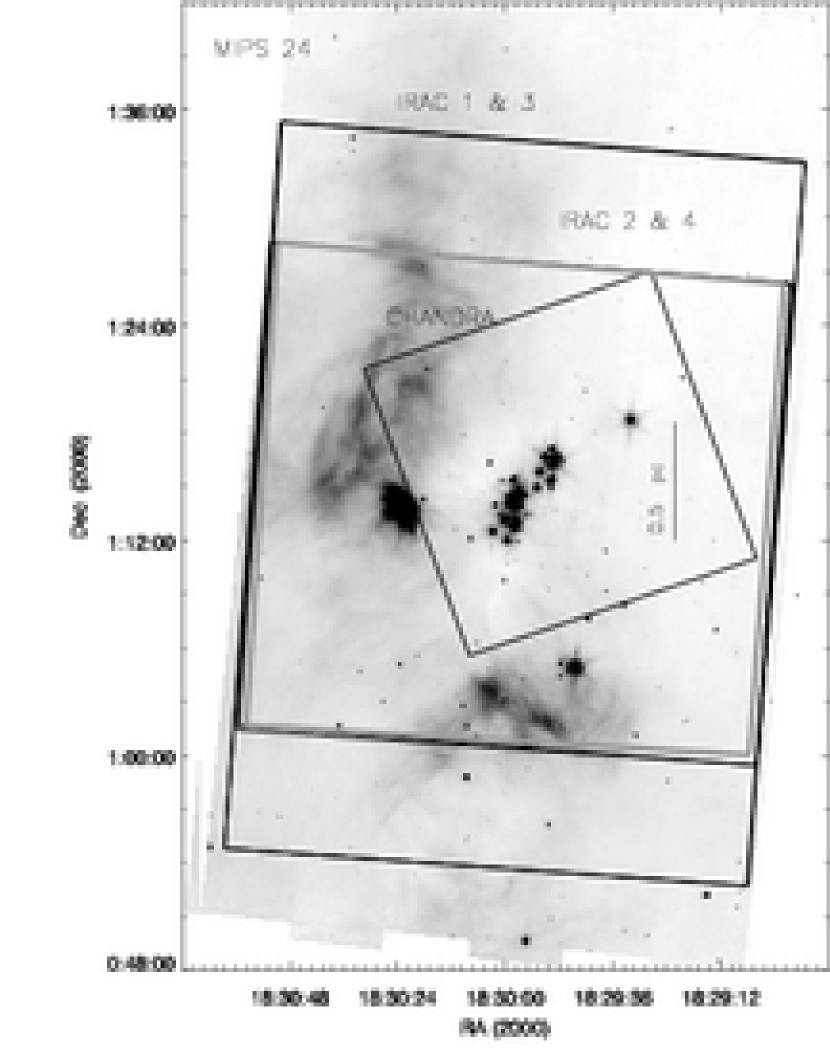
The field of view (FOV) of each instrument did not cover the same region of the cluster, being most limited by the IRAC FOV in the infrared, and overall by the Chandra FOV. The MIPS data covered the entire IRAC field, while the 2MASS survey is not spatially limited. Furthermore, the IRAC detectors are split into two groups, channels 1 & 3 (3.6 & 5.8 ) and channels 2 & 4 (4.5 & 8.0 ), whose FOVs are offset from one another by . The field studied in the remainder of this paper is the overlap region of all five Spitzer bands, the IR-field (Fig.3). The size of the overlap regions is 26′ 28′. In comparison, the Chandra image of Serpens covered a 17′ 17′ field of view (the IRX-field), centered on the northwestern edge of the cluster, 2′ from the center of the IRAC FOV (Fig. 3). X-ray data is not available for all the sources in our catalog.
5 Identification of Young Stellar Objects
The Serpens field contains 19,181 sources with a detection in at least one band with photometric uncertainty in the IR-field (122 having detections in all five bands); however, only a small fraction of these are bona fide YSOs. Three methods were applied to these data to identify possible young stellar objects: selection of stars with IR excesses on IR color-color diagrams, identification of X-ray luminous YSOs by comparison of X-ray sources with IR detections, and finally, a search for extremely red mid-IR sources among the detections.
5.1 Detection by InfraRed Excess
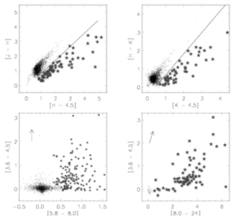
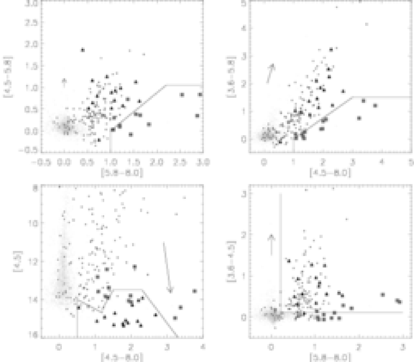
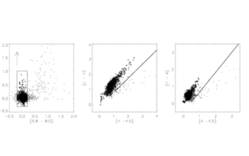
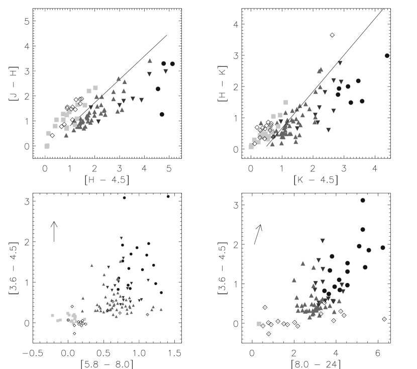
Young stellar objects can be identified by their excess emission at IR wavelengths. This emission arises from reprocessed stellar radiation in the dusty material of their natal envelopes or circumstellar disks. The infrared identification of YSOs is carried out by identifying sources that possess colors indicative of IR excess and distinguishing them from reddened and/or cool stars (Megeath et al., 2004; Allen et al., 2004; Gutermuth et al., 2004; Muzerolle et al., 2004). The main limitation of this method is the contamination from extragalactic sources such as PAH-rich star-forming galaxies and AGN; both of these have colors similar to young stellar objects. Four color-color diagrams were used to determine the color excess of the sources: an IRAC [3.6] - [4.5] vs. [5.8] - [8.0] diagram, an IRAC-MIPS [3.6] - [4.5] vs. [8.0] - [24] diagram, and two IRAC-2MASS diagrams J - H vs. H - [4.5] and H - K vs. K - [4.5], Fig.4. In the following analysis we required all photometry to have uncertainties mags in all bands used for a particular color-color diagram. The numbers of sources for each diagram which satisfy this criteria are 2417, 122, 3748, and 4251, respectively.
5.1.1 IRAC Color-Color Diagram
To identify sources with true IR excesses, it is necessary to distinguish between reddened or cool stars and those with excess emission arising from heated dust grains. A reddening law in the IRAC bands was determined by Flaherty et al.(2006), which shows the [5.8] - [8.0] color to be particularly insensitive to reddening and stellar temperature, and is thus a reliable measure of excess emission due to dust. Sources with a color beyond mag are likely to possess excesses and not to be reddened or cool stars (Fig.6).
Extragalactic sources such as PAH rich star-forming galaxies and AGN will also satisfy this criteria (Stern et al., 2005). Sources with a color more than below were considered galaxies and were removed; those with a 24 detection are reconsidered separately. Gutermuth et al.(submitted) have recently developed a method for substantially reducing extragalactic contamination built on the Bootes Shallow Survey data (Eisenhardt et al., 2004) and the Spitzer cores to disks legacy program methods (Jorgensen et al., 2006; Harvey et al., 2006) . The galaxies are eliminated either by their colors, which unlike YSOs are often dominated by PAH features in the 5.8 and 8.0 bands, or by their faintness. AGN are typically much fainter than the YSOs found in nearby star-forming regions and are removed by this criterion. It should be noted that very faint or embedded flat spectrum sources may be erroneously filtered by this method also. Fig.5 shows the color-color and color-magnitude diagrams used to identify star-forming galaxies with strong PAH emission and AGN.
Nebulosity may also result in the misidentification of sources. There are 55 sources with excesses in the [5.8]-[8.0] color, but little evidence of an excess in the [3.6]-[4.5] color. Examination of the spectral energy distributions for these sources (Sec. 6) showed that these sources exhibit excess emission only in the 8.0 band. Subsequent analysis showed that seventeen of these also showed excesses in the 24 band, but 38 showed no 24 detection. The seventeen 24 excess sources followed the distribution of the other bona fide YSOs in the field, while the 38 sources with weak 8.0 and no 24 excess were found in regions of bright 8.0 nebulosity to the East of the cluster (Fig. 2). These sources appear to have their 8.0 photometry contaminated by the nebulosity and were removed from the sample. In general, all sources with [5.8]-[8.0] excesses which do not show an excess at 24 excess or a are removed.
In total, 146 potential YSOs were identified in the IRAC color-color diagram. Of these, 62 are likely to be contaminants and have been removed from the source list.
5.1.2 IRAC-2MASS Color-Color Diagrams
The shorter wavelength 3.6 and 4.5 IRAC bands are much more sensitive to stellar photospheres than the longer wavelength 5.8 and 8.0 bands; where the shorter wavelength bands have 17,385 and 15,539 detections with , respectively, the longer wavelength bands having 4,670 and 2721 detections. Hence many sources cannot be characterized with the IRAC color-color diagram. For this reason, it is important to develop methods to identify sources with infrared excesses that rely only on the shorter wavelength bands. Since we cannot distinguish between reddening and infrared excess from circumstellar dust with only two bands, we combine the near-IR data from the 2MASS point source catalog with the 3.6 and 4.5 band photometry (Skrutskie et al., 2006). This provides the ability to detect objects which are too faint for detection in the 5.8 and 8.0 bands. In particular, we concentrate on the vs. diagram and the vs diagram. These diagrams take advantage of the excellent sensitivity of Spitzer in the 4.5 m band and the stronger infrared excess emission at 4.5 m compared to that at shorter wavelength (Gutermuth, 2005). For highly reddened sources which are not detected in the -band, the vs. diagram can be used. It should be noted that the IRAC 3.6 and 4.5 data can detect sources too faint or reddened to have been detected by 2MASS. Deeper near-IR imaging is needed to detect these sources in the , and -bands.
We calibrated the combined IRAC-2MASS color-color diagrams using a sample of stars which show no evidence for infrared excesses out to 8.0 , and which had uncertainties in all IRAC-2MASS bands, c.f. Fig. 6. They were identified primarily by their [5.8]-[8.0] color, which is not significantly affected by extinction (Flaherty et al. 2006). The criteria used were the following:
The [3.6]-[4.5] color was also limited to values less than one to eliminate contamination from protostars which can have [5.8]-[8.0] close to that of pure photospheres (Hartmann et al., 2005).
This sample of reddened photospheres was then plotted on the v and vs. color-color diagrams to define where the reddened photospheres fall in the diagrams (Fig.6). Reddening vectors derived from Flaherty et al. (2006) were placed on the diagrams so that all of the pure photospheres were blueward (to the left) of the vectors. Sources which were more than redward of the reddening vectors were selected as having an excess.
Using this analysis on the vs. diagram, the following criteria for infrared excess stars was established:
where 0.912 is the slope of the reddening curve. There were 72 sources detected using these criteria, 27 of which are not found with the IRAC color-color diagram. Of the 27, 12 were found to be contaminants.
In the vs. diagram, the infrared excess stars were identified using the following criteria:
where 0.873 is the slope of the reddening curve. There were 50 sources detected via this plot, 8 not detected on the IRAC or vs. color-color diagrams. Three of the eight were found to be contaminants.
There were 24 sources identified as having an excess on the IRAC-2MASS color-color diagrams that did not have photometry in all the IRAC bands and did not show a [3.6]-[4.5] color excess. In these cases, the observed infrared excess resulted from a discontinuity between the 2MASS and IRAC photometry; such a discontinuity may be the result of time variability or contaminated photometry. These sources were not selected as infrared-excess sources.
To minimize contamination from AGN, sources which lacked 5.8 and 8.0 detections and were identified solely in the IRAC-2MASS color-color diagrams were rejected if their 3.6 magnitude was fainter than 15 mag. At the distance of Serpens, this magnitude is well below the cutoff of the Hydrogen-burning limit for 1-3 Myr stars (12-13 mag; Baraffe (1998)). From our analysis of the IRAC color-color diagram (sec 5.1.1), sources identified as AGN dominate this region (Fig. 7).
5.1.3 IRAC-MIPS Color-Color Diagram
For young stars with circumstellar disks, the [3.6] - [4.5] vs. [8.0] - [24.] color-color diagram is very sensitive to the IR excess emission from dust at 3-5 AU (Muzerolle et al., 2004). It is particularly effective at identifying stars with little to no mid-IR excess shortward of 8.0 due to inner holes in their disks. These transition disks appear to be in a state of evolution where the inner disk has been cleared of small dust grains by planets or grain growth (Lin & Papaloizou, 1986). We used the following selection criteria:
A lower limit of 0.4 mag was used to conservatively eliminate pure photospheres even in the presence of photometric scatter due to nebulosity and source confusion. This criteria also excludes likely extragalactic sources which have colors [8.0] - [24.] (Muzerolle et al., 2004). A total of 75 young stellar objects were identified on these diagrams, 15 of which were not previously identified in the IRAC and IRAC-2MASS color-color diagrams. Three of the fifteen were identified as extra-galactic contaminants.
5.1.4 Completeness
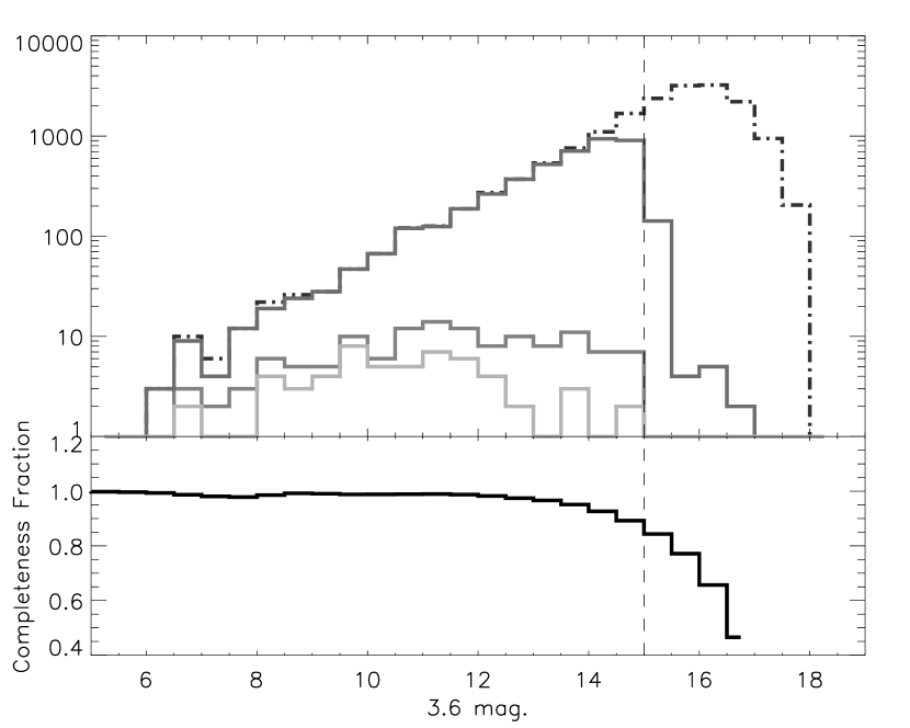
Estimates for the 90% completeness limit of our Spitzer photometry were calculated via the method of inserting artifical stars into the mosaics and then employing our detection algorithms to identify them. The 90% completeness estimates were 15.0, 15.0, 14.5, 12.5, 7.5 at 3.6, 4.5, 5.8, 8.0, and 24 , respectively, for the IRAC and MIPS photometry.
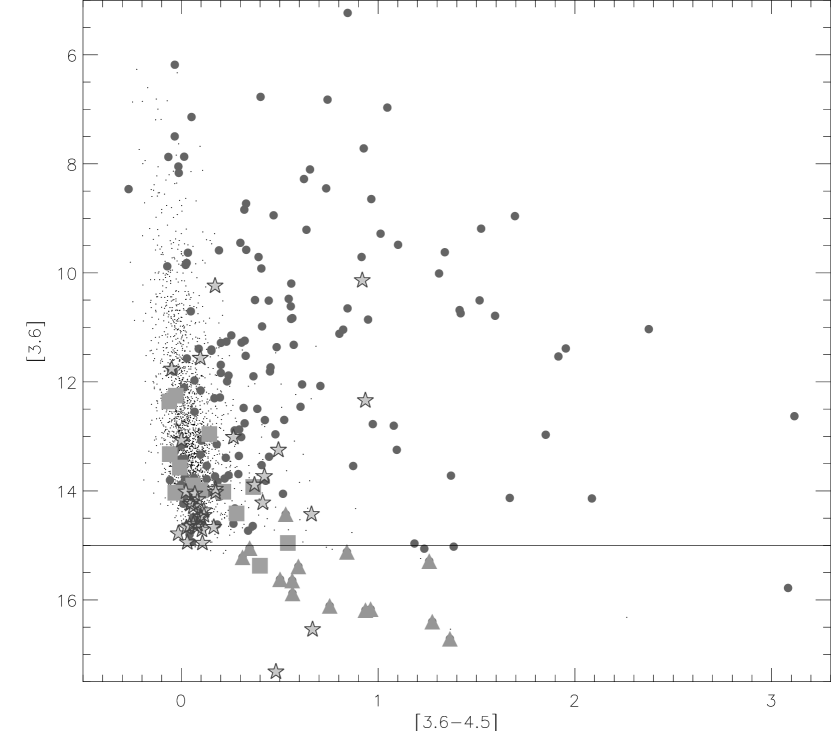
Fig. 8 plots the histograms and completeness of sources at 3.6 . The dashed black line plots the number of 3.6 detections by magnitude. We have also plotted the number of sources which have sufficient signal to noise in the relevant bands that they can be placed on the IRAC, IRAC-MIPS and/or IRAC-2MASS color-color diagrams (upper grey line). These are the sources which can be searched for IR-excesses. The final YSO catalogue sources are also plotted (lower gray line), as are the YSOs detected in X-rays (lower light gray line). The ratio of the number of sources with mag. that can be placed on the color-color diagrams to the total number of sources with mag. (and correcting this number for completeness by dividing by the fraction of artifical stars recovered in each magnitude bin) is or 81%.
The same ratio for detections above 14.5 and 14 magnitudes, the percentages are 93% and 97% respectively. These fractions represent lower limits on the completeness of the YSOs, as the number of contaminating field stars is rising with increasing magnitude, while the number of YSOs does not show an equivalent rise. Magnitudes of 14.5 and 15 for IRAC 3.6 , correspond to masses of 0.02 and 0.03 at 1 Myrs, and 0.03 and 0.04 at 3 Myrs (Baraffe, 1998). This completeness limit is for pre-main sequence stars with IR-excess emission from circumstellar disks. Since the fraction of sources with IR-excesses varies with mass and age (Lada, 1987; Hernadez et al., 2006), the completeness with respect to all pre-main sequence cannot be estimated with the available data.
5.2 II: Extremely Red Mid-IR Sources
Deeply embedded protostars may only be observable at 8.0 or 24 , and thus not be detected by the previous methods (Gutermuth et al., 2004). In order that these objects are not overlooked, the SED of each of the 24 detections that was not already selected was visually examined. Three sources were identified at 24 only, and one source was identified at 8.0 and 24 . One of sources detected at 24 lies at the position of a known sub-millimetre source, SMM1 (Testi et al., 1998); it is one of the brightest 24 sources on our image () and is also seen at 70 . Another source coincides with SMM8 (Testi et al., 1998); this is detected in both 8.0 and 24 . It is a fainter source, 11.5 mag at 8.0 and 6.3 mag at 24 . One of th esources is near the (sub)mm source SMM3, and is probably associated with that source. However, given the lack of clear detections in the IRAC-bands and the lack of a clearly identifiable 70 counterpart in this crowded region, we consider this 24 source a tentative YSO.
The remaining source, detected only at 24 , was detected in only one of the two epochs of MIPS observations, and is probably an asteroid.
5.3 III: X-ray Luminous Stars
Young stellar objects may also possess elevated levels of X-ray emission () which can be used to distinguish them from field stars (Feigelson & Montmerle, 1999; Feigelson & Kriss, 1981). We utilize this property to identify YSOs that do not have emission from a dusty disk (evolutionary class III) and would otherwise be indistinguishable from field stars. Protostars (class 0/I) and pre-main sequence stars with disks (class II) with elevated X-ray emission may also be identified. The Chandra image of Serpens covered a 17’ 17’ field of view centred on the cluster, and X-ray data is not available for all the sources in our catalog, c.f. Table 2.
The Chandra observations detected 88 sources in the region, a mix of genuine YSOs and AGN. The coordinates of these sources were matched against the 19,000 IR sources, with 67 matches, or 76%. The lower limit of the X-ray luminosity detectable in Serpens with Chandra can be estimated by comparison with the COUP data, see Feigelson et al. (2005), as , assuming a distance of 260 pc to Serpens and an exposure time of 88 ks. We match the X-ray sources with IR analogues to reduce the contamination from AGN; an X-ray source with no IR counterpart is assumed to be AGN contamination.
Of the 67 matches, 40 were IR excess sources previously identified, 3 sources had only been detected in some of the infrared bands and consequently could not be placed on the color-color diagrams used to identify infrared excess sources. The remaining 24 sources did not exhibit an IR-excess. Of the 67 IR matches, 27 of the X-ray luminous stars are not in the list of infrared excess sources. Of these 27 sources, five of the sources with Chandra and Spitzer detections were identified as probable AGN using the criteria in Sec 5.1.1. An additional two sources which did not show detections in all of the IRAC bands had 3.6 magnitudes fainter than 15; these seven sources were cosidered to be contaminating AGN. In total, 60 YSOs were detected in X-rays, 20 of which are new to the YSO catalog. The completeness of the X-ray data can be assessed from Fig. 8; it should be noted that only 78% of the YSOs from class 0/I to transistion disk lie in the IRX-field, thus the completeness of the X-ray data is limited partially by the smaller field of view. For we detect 57% of the YSOs in X-rays, this percentage drops quickly for fainter magnitudes. This corresponds to a mass of 0.18 for an age Myr and an (Baraffe, 1998).
5.4 Summary of Identified Objects
A total of 229 candidate objects were identified in the overlap IR-field through the methods outlined above. A list of 200 candidate members was compiled from the color-color diagrams, 66 were detected in X-rays in the IRX-field, and three as extremely red mid-IR objects. After contaminant removal there remained a total of 138, which we consider to be bona fide young stellar objects. The membership of Serpens is estimated to be more tahn 97% complete to 14 mag at 3.6 , or 0.04 at 1 Myrs (Baraffe, 1998), for sources with mid-IR excess emission. As will be shown, 50% of objects in each evolutionary class are detected in X-rays, thus we are likely missing 21 class III members in the IRX-field. By scaling the Harvey et al. (2006) results to our 0.2 field, we estimate that there is of order 1 AGB contaminant in our catalogue. We have removed 15 AGN and 13 galaxies with strong PAH-emission features, and estimate that 1 such contaminating object remains in the final source list (Gutermuth et al., submitted). We estimate that 1 or less of the class III sources may be a dMe contaminant. A list of the coordinates 137 of the sources identified as young stellar objects in the Serpens Cloud Core is given in Table 4 with associated identifiers. The photometry of the sources is given in Table 5. These two tables do not list the photometry for two sources detected only by MIPS, SMM1 and SMM3, whose fluxes are listed in Table 6. Since SMM3 is only clearly detected by Spitzer at 24 , we have not included SMM3 in the 138 sources.
6 Evolutionary Classification
The evolutionary state of a young stellar object can be inferred from the Spitzer mid-infrared photometry (Allen et al., 2006). The classification of the Serpens sources was carried out using four different diagnostics: mid-IR colors (Allen et al., 2004; Megeath et al., 2004), the slope of the Spectral Energy Distribution (SED) (Gutermuth et al., 2004), the dereddened SED slope, and the shape of the SEDs (as ascertained by visual inspection). Each source was classified as either class 0/I, flat spectrum, class II, transition disk, or class III (Lada & Wilking, 1984, see following subsections for the definition of these classes).
Classification of the sources was carried out by first noting their locations on the IRAC, IRAC-2MASS and IRAC-MIPS color-color diagrams and assigning each source a preliminary class (Megeath et al. (2004); Allen et al. (2004); Gutermuth et al. (2005); Muzerolle et al. (2004), see Fig. 9). Typically, the IRAC color-color diagram was used for the initial assignment of the evolutionary class. An exception was made in the case of the transition disk objects which do not always possess an 8.0 excess and are most clearly identified by their [8.0] - [24.] color from the IRAC-MIPS diagram.
This was followed by the construction of SEDs for all sources. Examples of the SEDs for the different evolutionary classes are given in Fig.10. For each SED, a slope was calculated. The conversion from magnitudes to fluxes in W cm-2 s-1 used the following zero fluxes for the , , , [3.6], [4.5], [5.8], [8] and [24] bands respectively: . The slope was calculated by a least-squares fit over the available IRAC bands, and where possible IRAC and MIPS. The near-IR magnitudes were not included as they are most susceptible to extinction.
The Serpens cluster contains many deeply embedded members with extinctions reaching 40 . For sources with detections in at least two of the near-IR bands, we have measured the extinction using a method developed by Gutermuth (2006). This method uses the extinction law of Flaherty et al (2006) and the YSO loci from Meyer et al. (1997) and Gutermuth (2006) to determine the extinction and deredden the sources. The slope of the SED of the dereddened source was also measured.
In the majority of cases the SED slope and color-color diagram methods agreed (118, 86%). Where they did not, further examination was undertaken to ascertain where the discrepancy arose: 18 members (14%) were classed differently via the IRAC and the dereddened SED methods. Visual inspection of these objects was carried out to better distinguish their class. In 17/18 cases the class derived from the dereddened data was the final choice. The remaining two objects were detected at 8.0 and 24 , and 24 only, and are coincident with known (sub)mm protostars.
6.1 Class 0/I Protostars
Class 0/I sources are protostellar objects surrounded by in-falling dusty envelopes. They are characterized by rising SEDs in the infrared (Lada, 1987). The standard criteria, that class 0 sources with (Andre et al., 1993), cannot be established from the Spitzer data. As some known class 0 sources have been detected with Spitzer we refer to all sources showing rising SEDs as class 0/I objects (Hatchell et al., submitted). These sources were identified in our data by their rising SEDs (; note we used the 3.6-24 slope when available, these may be different to the 3.6-8.0 slopes listed in Table 5), and by satisfying one of the two following criteria: (Allen et al., 2004; Megeath et al., 2004):
There can be some overlap between highly reddened class II sources (stars with disks) and class 0/I objects (Whitney et al., 2003b). To distinguish between these sources, we used the dereddened SEDs. Sources that showed dereddened SEDs that looked like other class II sources were deemed class II. These objects are found in the class 0/I region of the IRAC color-color diagram in Fig. 8. Although all class 0/I objects might be thought of as class II like objects reddened by their protostellar envelopes; the envelope also results in the scattering of a significant component of light in the near and mid-IR (Kenyon et al., 1993; Whitney et al., 2003a; Doppman et al., 2005). In addition, there may be a contribution from thermal emission from the inner envelope. For this reason, class I objects cannot be simply dereddened, and the application of our dereddening algorithm results in SEDs which appear distinctly different than the class II objects (see Fig. 9). In total, 22 class 0/I protostars were identified.
6.2 Flat Spectrum Objects
Flat spectrum sources possess a ’flat’ SED () (Greene et al., 1994), they do not exhibit the steeply rising SED of protostars (class 0/I), but the have too much excess for it to arise simply from a circumstellar disk (class II). Flat spectrum sources are thought to be an intermediate phase between the class 0/I and class II phase where the central star and disk are surrounded by a thin infalling envelope (Calvet et al., 1994). Initially 26 objects were tentatively classified as flat spectrum sources, using the undereddened , many because they lacked the necessary near-IR bands to further constrain their classification. This class is particularly sensitive to contamination from AGN, as both have similar colors. Each flat spectrum object was individually examined, and where possible its dereddened slope was used, to distinguish between class 0/I (), class II (), and flat spectrum, (). We used the 3.6-24 slope for sources with 24 detections; in other cases we used the 3.6-8.0 slope () given in Table 5. Finally, the locations of all the flat spectrum members were plotted on the IRAC color-color diagram; these sources delineated the boundary between the class 0/I and II objects (Fig. 8). In total, 16 flat spectrum objects were identified.
6.3 Class II
Class II sources are identified by having an (Greene et al., 1994; Andre et al., 1994), and the following mid-IR colors (Allen et al., 2004; Megeath et al., 2004):
Note that we have lowered the minimum slope from -1.6 to -2 in order to contain evolved or anaemic disks found in other star forming regions (Lada et al., 2006; Hernadez et al., 2006). The class II members were refined by addition of the reddened class II objects initially classed as protostars: in total 8 sources (6%) were reclassified from class 0/I to class II. Class II sources from the IRAC-2MASS diagrams were distinguished from protostars by their slopes in the available IRAC bands. In total, 62 class II stars were identified.
6.4 Transition Disks
Seventeen sources were plotted that had an excess at 8.0 and/or 24 but none at shorter IRAC wavelengths.
These sources are considered to be transition disk objects, stars with a cleared inner disk but retaining an outer disk starting at a few AU (Muzerolle et al., 2004; McCabe et al., 2006). It is thought that the inner disk might be cleared due to formation of planets or the agglomeration of the dust particles into larger mm-sized grains (Calvet et al., 2002; Lin & Papaloizou, 1986; Muzerolle et al., 2004). Those with weaker excess () may be debris disks (Muzerolle et al., 2004). Identification of these objects by SED slope is unreliable, due to the jump in flux at the longer wavelengths (Fig. 9). Visual examination of the SED must be carried out to verify that they show excess only longward of 8.0 . They tend to lie near the lower boundary of the class II region on the IRAC color-color diagram, showing little or no excess on the [3.6] - [4.5] color-axis and varying degrees of excess along the [5.8] - [8.0] color-axis (Fig. 8). They are more reliably identified using the IRAC-MIPS color-color diagram (Fig. 8). In total we find 17 transition disk candidates. An additional 3 sources were initially classed by their mid-IR color excesses as Class II sources, but were identified as transition disk objects from the lack of excess shortward of 24 in their dereddened SEDs. These sources appear in the Class II region in the IRAC and IRAC-MIPS color-color diagrams. (Fig. 8). There is a possible source of contamination in the transition disk sources: AGB stars, which have similar colors (Blum et al., 2006), with . This affects eight of the sources, spectroscopy will be needed to determine whether these sources are contamination or members.
6.5 Class III
Class III objects are pre-main sequence stars which do not have circumstellar disks detectable in the mid-IR. They exhibit colors in the color-color diagrams consistent with reddened photospheres, an SED which approximately follow a Rayleigh-Jeans law (Lada, 1987), and exhibit no excess in the mid-IR. In total, 21 of the X-ray identified YSOs were found to be class III. We cannot distinguish between class III stars without elevated X-ray emission and field stars in the line-of-sight. Considering both the smaller field of view of the Chandra observations and the fact that only a fraction of young stars show elevated X-ray emission (see the X-ray discussion in Sec 7.4), a substantial number of unidentified class III objects may exist in the cluster. Further spectroscopic information on stars in the field will be required to positively identify these Class III sources.
7 Discussion
We have identified 138 young stellar objects: 22 class 0/I objects, 16 flat spectrum sources, 62 class II objects, 17 transition disks, and 21 class III objects. In the following discussion we use this sample to address four topics. First, we compare our results to previous studies of the Serpens embedded cluster. Second, we identify Spitzer analogs to sub-millimeter sources previously found in this region. Third, we study the spatial distribution of the sources as a function of their evolutionary class. Finally, we discuss the X-ray properties of the YSOs detected in the Chandra X-ray observavtions.
7.1 Previous Infrared and X-ray Studies
Eiroa & Casali (1992) observed the Serpens cluster in the J, H, K, and nbL bands and identified 50 young stellar objects in the region. We match all 50 sources to detections in our overlap region, although an offset of up to 9′′ was needed to identify their counterparts in our data. Of the 50 sources, 34 have been identified as YSOs in our analysis. The remaining sixteen sources were found to have IRAC colors of reddened stellar photospheres without infrared excesses or to have too few bands to classify reliably, and none of these sixteen sources showed X-ray emission. These sources cannot be established as YSOs by our criteria.
A previous study by Kaas et al. (2004) using the ISOCAM instrument on-board ISO, identified 77 cluster members in a 0.13 region centred on the Serpens core, at wavelengths of 6.7 and 14.3 . Of these, 70 matched with a Spitzer detection in the IR-region, with the remaining 7 outside of the overlap region but detected in one or more Spitzer bands. A maximum offset of 9′′ was used to match the sources to our data. Of the 70 sources, 56 are identified as YSOs in our final catalogue, while the remaining 14 were found to be reddened stellar photospheres without infrared excesses or X-ray detections. These remaining 14 were not identified as YSOs in our analysis. Of the YSOs in common with Kaas, two of our class II objects are classified as class I by Kaas and one of our class III objects is classified as class II by Kaas.
A previous study of the Serpens Core was undertaken in X-rays by Preibisch (2003) and Preibisch (2004) with the XMM-Newton Satellite. In one observation of ks and two observations of ks each over and energy range of 0.15-5 keV, 47 sources were detected; 4 class I, 2 flat spectrum, and 41 class II young stars. These observations are not as deep as the 88 ks Chandra integration, and do not possess as high an angular resolution. We detect a total of 60 X-ray sources in the Chandra data, 13 more members than the Preibisch study. Twelve of these newly discovered X-ray sources are class 0/I or flat spectrum sources, indicating that the Chandra observations are detecting more deeply embedded X-ray sources.
Eiroa et al. (2005) describes VLA 3.5cm observations of the Serpens Core, identifying 22 sources, thirteen of which matched to infrared counterparts. Nine of these are class 0/I sources including SMM1 and SMM5, one is a flat spectrum, two are class II and one is class III. Three further sources were matched to counterparts detected in one or two bands only. The class III object is detected in the X-ray, thus all thirteen sources have one of our two criteria for membership: an infrared excess and/or an infrared counterpart (with or without an excess) to an X-ray detection. The remaining six sources without infrared counterparts are most likely background sources which are too faint and/or reddened to be detected in the 2MASS or Spitzer infrared data. The fluxes of the VLA sources coincident with the protostars detected in the (sub)mm are given in Table 6. Eight of the 13 VLA sources with infrared counterparts have Chandra X-ray counterparts as well; hence, 60% of the VLA sources are detected by Chandra. In comparison, in the Ophiuchus core (165 pc), 8/28 or 36% of the VLA sources had both X-ray and infrared counterparts (Gagne et al., 2004). In the Coronet cluster (140 pc), 9/15 or 60% of the Radio sources have been detected in multi-epoch analysis of X-ray data (Forbrich et a., 2006). The measurements are consistent within the statistical uncertanties of the ratios, even though the sensitivities vary substantially; the X-ray detection rates in the Coronet cluster were found in 20 ks observations, while the Oph core observation was nearly 5 times longer.
Giardino et al. (2006) have recently submitted the results of the Chandra observations of the Serpens cluster. This work was done in collaboration with our team, and they have reported the evolutionary classes listed in this paper. Table 4, listing the coordinates and identifiers of the YSOs, provides the cross reference for the Giardino et al. (2006) source numbers in the eighth column.
Harvey et al. (2006) presents IRAC observations of the Serpens cloud as part of the Spitzer Legacy project ”From Molecular Cores to Planet-forming Disks” (c2d; Evans et al. (2003)). The surveyed area covers a much larger field of deg2 than covered in this paper. They identified 257 young stellar objects throughout the field, in two main groupings. One, labeled ’A’ in Harvey et al. (2006), is the Serpens main core cluster studied in this paper, the second region, cluster ’B’, being about to the south of the main core. An important difference between this work and that of Harvey et al. (2006) is the selection of class III objects. The Harvey et al. (2006) criterion for class III sources required an ; their class III objects are sources with weak infrared emission from a disk that we would classify as a weak class II or transition disk object. In contrast, our class III sources are defined as lacking in infrared emission yet exhibit detectable X-ray emission. Bearing this in mind, the numbers of class I, flat spectrum, class II, and class III members identified in their larger field were 30, 33, 163, and 31, respectively.
7.2 Protostars in the Serpens Clusters
The number of young stellar objects identified is 138. There are 38 protostars (22 class 0/I, 16 Flat Spectrum) and 100 pre-main sequence stars (62 class II, 17 transition disks, and 21 class III). Protostellar class 0/I and flat spectrum sources account for 28% of the YSOs detected. The ratio of protostars to pre-main sequence stars with disks is 48%; this high number indicates that Serpens is unusually rich in protostars, and is in agreement with the 56% fraction found in Kaas et al. (2004). Over the entire Serpens cloud, the ratio was found to be 38% (Harvey et al., 2006). In comparison, the fraction of protostars to stars with disks detected with the Spitzer Cores to Disks (c2d) survey was 14% in the IC 348 cluster and 36% in the NGC 1333 cluster (Jorgensen et al., 2006), and 50% in Chameleon II (Porras et al., 2007).
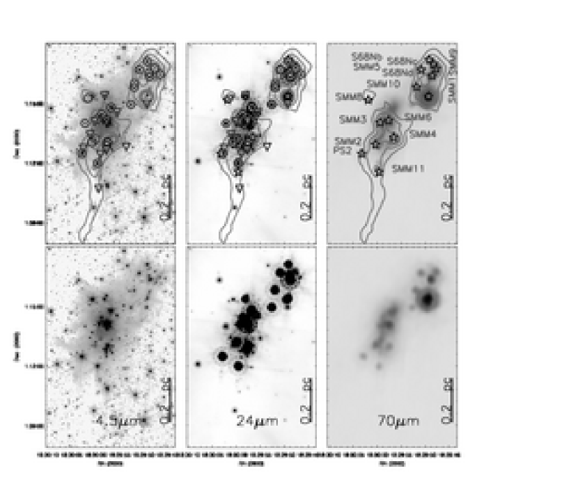
Previous observations at sub-millimeter and millimeter wavelengths have identified a number of presumably protostellar sources in the Serpens cluster. Studies by Testi et al. (2000), Davis et al. (1999), and Williams & Meyers (1999) identify fourteen objects detected at wavelengths of 3 mm or 850 m with flux densities greater than 3 mJy beam-1, and significance above 5 . Table 6 lists these objects with their identifiers, coordinates, and fluxes from the above mentioned papers combined with our Spitzer photometry. These are also shown in Fig. 11. We now discuss these sources:
SMM1: At the location of SMM1 we find a bright 24 and 70 source. Outflow knots associated with SMM1 are visible in our 4.5 IRAC mosaic, and diffuse emission is visible in the 8.0 ; however, we do not identify a compact source at this location. This appears to be a umambiguous example of a Class 0 object too deeply embedded to be detected shortward of 24 .
SMM2: Two Spitzer identified class 0/I sources are found within of the SMM2 source; these sources appear to be beyond the positional uncertainties in the 3 mm data () and are not coincident with SMM2. There is also 70 m emission in the region around SMM2, it is not clear which of the three sources (SMM2 and the two class 0/I) contribute to 70 m emission. Interestingly, there is a faint slightly extended 4.5 m source toward the position of SMM2. This suggests that the SMM2 source may be a protostellar source with associated infrared emission, although the lack of 24 m emission is puzzling.
SMM3: There is a 24 m source within of the location of SMM3, which we tentatively assign to it. While there is extended 70 m emission in the region of SMM3, no point source could be photometered due to flux contamination from nearby bright sources. While there is faint emission towards this source in the IRAC bands, it is confused with image artifacts from neighboring bright sources.
SMM4: There are no sources identified in the IR coincident with SMM4, but two small areas of nebulosity can be seen in the 4.5 image. Again, this suggests that a protostellar source may reside in SMM4, but if so, there is a lack of bright 24 m and 70 m emission from the source.
SMM5, SMM9, S68Nb, S68Nc and S68Nd: These five sources are associated with the group of four class 0/I objects on the northwestern side of the cluster. In addition, the outflow jet associated with object S68Nc is visible in the IRAC bands. This region has previously been considered devoid of more evolved pre-main sequence stars, however we have identified two class II members in the vicinity.
SMM6, SMM8, SMM10, PS2: There is a flat spectrum source at the position of SMM6 and class 0/I objects at the positions of SMM8, SMM10 and PS2. Recent work by Haisch et al. (2006) identified SMM6 as the primary component of a double system. We do not see the companion in our data, as it is contaminanted by the flux from SMM6 itself.
SMM11: While there is no IR counterpart at the position of SMM11 from Testi et al. (1998), a class 0/I object north of its position is detected out to 70 m. We also note that the peak of SMM11 in the SCUBA 850 data is southeast of our class 0/I source and northwest of the Testi source. While it is possible that these are three separate objects, it seems unlikely; the position of this source needs to be re-examined in subsequent submillimeter observations.
Of the fourteen (sub)mm objects, seven correspond directly to sources detected in the IRAC bands, three are detected only with MIPS, and four are not detected at m. With the exception of SMM11, all of the (sub)millimeter sources are coincident with 70 m emission; however, the low angular resolution of the 70 m map () makes it difficult to extract the 70 m photometry for an individual source. In seven of these sources, the 70 m flux can be extracted; these fluxes are tabulated in Table 6 and the resulting SEDs are shown in Figure 12. For the remaining sources, the 70 m emission is too confused to photometer accurately. Three of the fourteen sources have X-ray detections in our data: SMM5, SMM6, and S68Nb. These appear to be Class I sources in that they show bright emission shortward of 24 m; there is no detectable X-ray emission toward the sources with weak or no detected emission shortward of 24 m, i.e. the probable Class 0 sources.
7.3 Spatial Distribution
The spatial distribution of young stellar objects in a cluster gives insight into the fragmentation processes leading to the formation of protostellar cores and the subsequent dynamical evolution of the stars as they evolve from the protostellar to the pre-main sequence stage (Allen et al., 2006). Recent work has shown that in many clusters the sources trace the underlying molecular gas distribution (Gutermuth et al., 2005). Kaas et al. (2004) made the first maps of the distribution of class II and class I objects in Serpens, demonstrating that the class I sources were significantly more clustered than the class II sources.
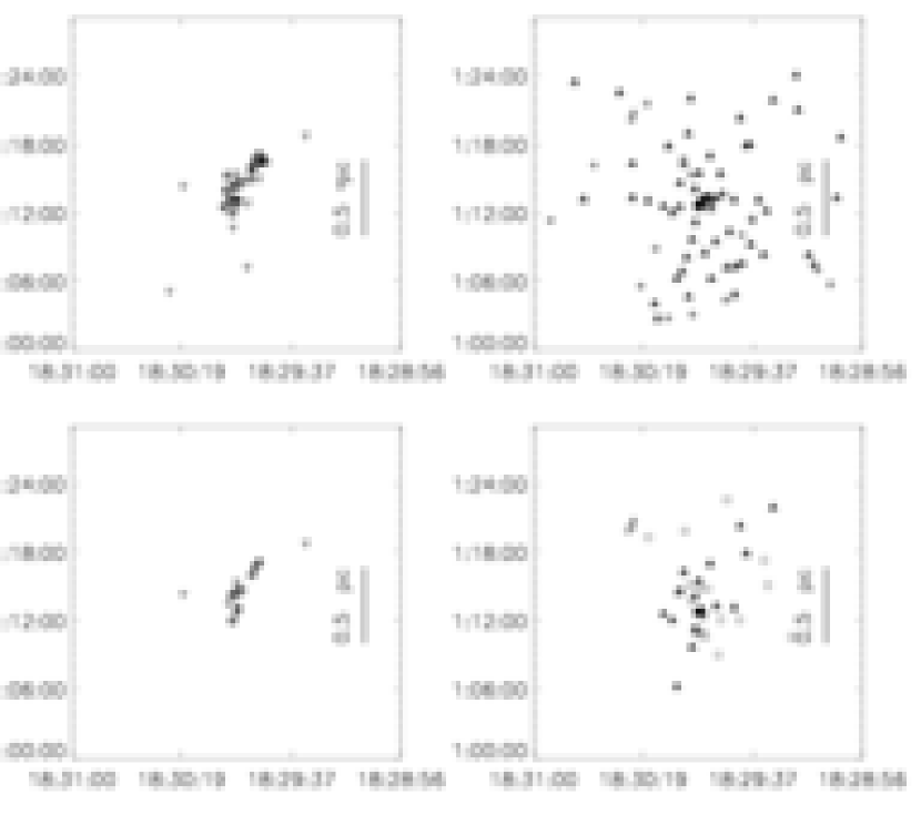
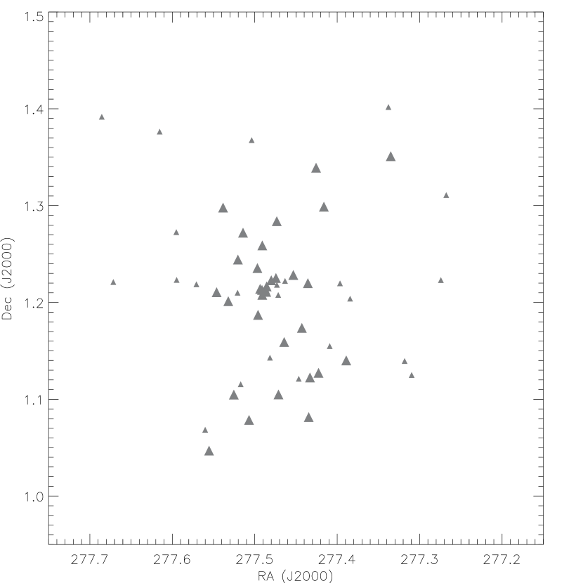
Fig. 13 shows the distribution of young stars as a function of their evolutionary class. This is shown for the sample of IR-excess stars and the sample of X-ray luminous stars. The most significant difference is between the class 0/I and flat spectrum sources, which are concentrated in a narrow filament in the center of the cluster, and the class II sources. Although there is a peak in the class II density in the center of the cluster, the majority of the class II sources, as well as the transition disk and class III sources, are found in an extended halo surrounding the protostars.
The protostars are coincident with the dense molecular ridge mapped by the 850 SCUBA map of Davis et al. (1999, 2000). The class 0/I and flat spectrum sources concentrated in two groups coincident with the two dominant molecular gas clumps (Fig. 11), confirming the previous work of Testi et al. (2000) and Kaas et al. (2004). These are coincident with the column density peaks of the 850 m map and have size 0.2 pc in diameter. The northern group contains 9 Class 0/I and 1 flat spectrum source, seven of which are found in a region only 0.1 pc in diameter, and 4 class II sources. The southern group contains a mixture of 12 class 0/I, 10 flat spectrum, 16 class II, 1 transition disk, and 5 class III sources in a pc diameter region. In the southwestern quadrant of this grouping is a small wishbone shaped sub-grouping. This sub-grouping of stars contains eight stars in an area 0.1 pc in diameter; including three class 0/I objects, one flat spectrum source and four class II sources. The higher fraction of class II sources in the southern group suggests that it is more evolved than the northern group. Finally, the X-ray data shows a grouping of four class III objects in the southwestern quadrant of the cluster within a 0.1 pc diameter region. This grouping is unusual in that it is the only apparent group of class III objects; all of the remaining class III objects are scattered around the cluster. If this is a bona fide group and not a chance alignment, it is of great interest why these objects have dispersed their circumstellar material.
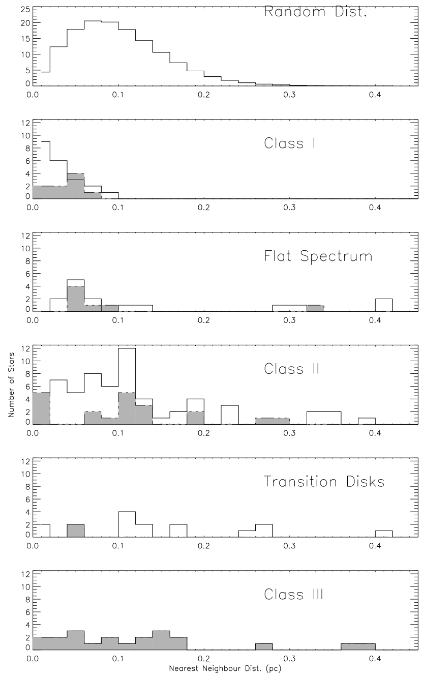
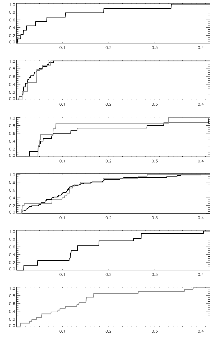
The spatial distribution of the cluster sources was examined for each of the five evolutionary classes using a nearest neighbour technique. The nearest neighbour distance is the projected distance to the nearest YSO of the same evolutionary class, using the adopted distance of 260 pc. Figure 14 (left) shows the distribution of nearest neighbour distance between the members of each class. The class 0/I sources are by far the most densely clustered, with a median separation of 0.024 pc. In comparison, the median nearest neighbor distances of the remaining evolutionary classes are significantly greater: flat spectrum - 0.079 pc, class II - 0.097 pc, transition disks - 0.132 pc and class III - 0.131 pc. The median distances for the flat spectrum and transition disk are biased to higher values by the small numbers (and hence low densities) of these sources. The class III sources mean distance may be biased to a lower values by the limited field of view of the Chandra data. These scales are smaller than the 0.12 and 0.25 pc separations for class I and II previously derived from ISOCAM observations (Kaas et al., 2004), which were limited by the lower angular resolution of ISO. Also plotted in Figure 14 are the cumulative distribution curves for the YSOs by class, showing how densely the sources are distributed over the field. A Kolmogorov-Smirnov (K-S) test was performed to ascertain the probability that they are derived from the same parent distribution. The Class I sources are dissimilar to each of the other classes, reflecting their more highly clustered nature (Table 3). The distributions of the four remaining classes are statistically indistinguishable (Table 3).
For each evolutionary class, 10K random distributions of stars were generated, with the number of stars equal to the number of objects in the given evolutionary class. For the class III sources, the randomly distributed stars were constrained to fall within the IRX-field, for all other classes, the random distribution covered the region of the IR-field that contained 90% of the sources. The resulting nearest neighbor distributions of the observed YSOs and the random distributions were compared for each class using the K-S test. The probabilities that the random and observed distributions were drawn from the same parent distribution were calculated for all 10K distributions; the mean values of the probablilities for each class are listed in Table 3.
Our results indicate that the median projected spacing of protostars in Serpens sources is only 5000 AU, and the spacing is as close as 2000 AU in certain regions such as the wishbone and the northern group. The actual physical spacings are probably larger; if we assume the sources are randomly distributed relative to each other, the median spatial separation between sources would be AU. If we assume that each protostar will form an 0.5 star, then for dense core densities of and cm-3 (Jijina et al., 1999; Olmi & Testi, 2002), such a protostar would have to accrete from a volume 12,000 and 4000 AU in diameter, respectively. Thus, assuming volume densities typical of dense molecular cores, the accretion volumes would be densely packed if not overlapping.
Is the observed spacing consistant with Jean’s fragmentation? The Jean’s length is given by (Jeans, 1928): . If we set the Jean’s length to be pc, adopt temperatures of 12 and 17 K (Jijina et al., 1999), and solve for the density, the resulting densities are cm-1 and cm-1. The observed gas densities range from cm-3 to cm-3 (Jijina et al., 1999; Olmi & Testi, 2002). Thus, the observed median separation is consistant (i.e. within a factor of two) with Jeans fragmentation given the highest observed densities in Serpens. At these highest observed densities, the spacing would also be approximately equal to the radius of a critical Bonner-Ebert sphere () (Ebert, 1955; Bonner, 1956). In either case, the spacing of objects at the Jeans spacing and Bonner-Ebert radius further indicate that the volumes of gas accreting onto the protostars are tightly packed or overlapping. We note that unlike the case of Teixeira et al. (2006), there is not a well defined peak in the distribution of nearest neighbor separations; many objects are found at separations much smaller than the median separation. This is in keeping with Young et al. (2006) who resolved one of the Teixeira et al. sources into a multiple system.
The close spacing of the protostars raises the possibility that competitive accretion is taking place. In competitive accretions models, several protostars accrete from a common reservoir of gas. These objects compete for gas from the reservoir; this process can lead to a distribution of masses similar to the initial mass function (Bate & Bonnell, 2005). In models of competitive accretion, protostars accrete mass through a Bondi-Hoyle accretion at a rate of
where is the volume density of the gas, is the instantaneous mass of the accreting protostar, is the sound speed of the gas and is the velocity of the star relative to the gas (Bondi & Hoyle, 1944; Bonnell & Bate, 2006; Shu, 1992). Williams & Meyers (2000) measured the velocities of 5 of the protostars in the northern group by using detections in the () line conicident with the protostars. The RMS 1-D velocity dispersion of these protostars is 0.26 km s-1, implying a 3-D velocity dispersion of 0.45 km s-1. Assuming a density of cm-3, a velocity of 0.45 km s-1, and a kinetic temperature of 17 K (implying a sound speed of 0.22 km s-1), for a protostar with a mass of 0.1 M⊙, the Bondi-Hoyle accretion rate is M⊙ per year, and for a protostar with a mass of 0.5 M⊙, the accretion rate is M⊙ per year. Given these accretion rates, adopting a protostellar lifetime of 300,000 (Hatchell et al., submitted), and considering that the rate will increase as the object grows in mass, the young protostars in the northern group could accrete a significant portion of their ultimate mass through Bondi-Hoyle accretion. Consequently, competitive accretion remains a viable process for the formation of stars in the Serpens cluster.
Finally, the close spacing and velocities of the protostars in the northern group suggest that their envelopes could impinge on one another. We note that the 3 mm continuum observations ( beamsize) of Williams & Meyers (2000) did not resolve the the sizes of the protostars in the northern group of Serpens. This does not rule out our previous estimates that the accretion volumes extend 5000 to 10,000 AU; the BIMA measurements may only be sensivite to dense inner regions of the protostars. However, for the present analysis, we use a size of 1000 AU, assuming that the protostars are spheres with diameters just below the angular resolution of the BIMA observations. We follow the analysis in Gutermuth et al. (2005), adopting a mass of 0.5 M⊙, a velocity of 0.26 km s-1 and a peak density for the northern group of seven protostars in a volume 0.1 pc in diameter. The resulting time between collisions for a given object is 200,000 years, less than the protostellar lifetime. Consequently, if the objects in this group remain in bound orbits within this region for 300,000 years, the typical protostellar lifetime (Hatchell et al., submitted), all of the protostars could experience collisions between their envelopes and the envelopes of other protostars in the group.
In summary, Jean’s length, Bonner-Ebert sphere and simple volumetric arguments all suggest that the accreting envelopes around the protostars in Serpens are often tightly packed, if not overlapping. We find that for the conditions present in the northern group, the protostars may accrete a significant amount of their mass through Bondi-Hoyle accretion from a common envelope, and competitive accretion may occur within the group. Furthemore, collisions between the sources are likely. In total, our analysis suggests that the interactions between protostars can play an important role in the formation of stars within the dense groups observed in Serpens.
7.3.1 The Substellar Candidates and their Spatial Distribution
Using the models of Baraffe (1998) we calculate the magnitude of the hydrogen burning limit at K-band to be 12.5 mag for an assumed 1 Myr old cluster at a distance of 260 pc to Serpens. Of the 138 sources in Serpens, 34 have K-band detections fainter than 12.5 magnitudes, 2 of which are class 0/I and one flat spectrum. Since we cannot measure the dereddened photospheric luminosities of the class 0/I and flat spectrum objects, these sources are discounted, leaving 31 candidate (23 class II and 8 class III) brown dwarfs members. Harvey et al. (2006) has also identified numerous substellar candidates in the Serpens ’B’ cluster to the south of the core. We cannot rule out that these sources are older objects or objects that appear underluminous for other reasons (Peterson et al., submitted; Slesnick et al., 2004). Searches for brown dwarfs in other regions have shown that infrared spectroscopy is essential to confirm that faint objects are protostellar in nature (Luhman, 2001). Assuming that the 23 class II objects were to be positively identified as substellar, this would lead to an upper limit of 23/138 or 17% of the total YSO population being substellar. This would be somewhat higher than the substellar fractions found in Chameleon 1 (5%) and IC348 (8%) (Luhman, 1999, 2005), though in agreement with Kaas et al. (2004), who estimate 20% of Serpens sources are substellar.
Interestingly, the spatial distribution of the 12.5 class II objects appears more extended that the brighter class II (Fig. 15). In particular, although smaller in number, the most distant objects north, west, and east of the core of the cluster have 12.5. This may be biased by the high reddening in the centre of the cluster which would preclude detections of faint objects in the near-IR. Using deeper near-IR photometry of the center of the cluster Kaas et al. (1999) also found that sources with dereddened 12.5 were non-centralised. Spectroscopy of the fainter objects is needed to confirm their substellar nature.
7.4 X-ray Characteristics
In recent years many studies have been undertaken to investigate the emission properties of pre-main sequence stars and protostars in the higher energy X-ray region of the spectrum (Wolk et al., 2006; Getman et al., 2005). In developed, hydrogen burning stars, X-ray activity arises from magnetic fields generated as a result of shear between the core radiative zone and the outer convective zone. The process behind the generation of the highly increased levels of emission in young stellar objects remains uncertain; suggested causes being magnetic disk-locking between the star and disk (Hayashi et al., 1996; Isobe et al., 2003; Romanov et al., 2004), accretion onto the star (Kastner et al., 2002; Favata et al., 2003, 2005), and alternative dynamo models for coronal emission (Küker & Rüdiger, 1999; Giampapa et al., 1996). In main sequence stars, there is a trend of decreasing X-ray activity with age; this trend has not yet been conclusively shown for pre-main sequence stars. Chandra has recently examined the X-ray properties of the Orion Nebula Cluster (ONC), in a project known as the Chandra Orion Ultra-Deep Project (COUP). Although the Serpens sample is much smaller than the COUP survey, the analysis of Serpens has the advantage of excellent 3.6-24 photometry; observavtions longward of 4.5 are difficult in the center of the ONC due to the bright infrared emission from the molecular cloud. This photometry allows us to accurately ascertain the evolutionary class of each object, and study the dependence of the X-ray properties with evolutionary state. Only those detections with X-ray count in excess of 100 were considered when examining emission properties to ensure reliable estimates.
Of the 138 identified members, 60 were conclusively shown to exhibit X-ray emission. Nine of the X-ray detections are associated with Class 0/I sources (43% of class 0/I’s in IRX-field), a further eight with flat spectrum members (56%). Twenty detections have class II counterparts (45%), while two of the transition disks are detected in X-rays (25%). The remaining 21 sources did not exhibit an IR-excess and were identified as a class III YSO solely on their X-ray emission; hence, 21/138 or 15% of the sources were identified solely by Chandra. There appears to be no evidence that the detection rate depends on evolutionary class; within 1 , the detection rates of class 0/I, flat spectrum, and class II sources are identical. The detection rate may be largely a function of the sensitivity of the Chandra observations; the majority of T Tauri stars have (Preibisch et al., 2005) while our sample is complete to . Since we cannot identify class III sources without X-ray emission, we cannot establish the fraction of class III sources detected in X-rays. As we will argue subsequently, the X-ray properties of the class II and lII objects appear to be indistinguishable. Assuming that this similarity holds for the fraction of detected sources, then the fraction of classs III sources detected is the same as that for the class II objects, and we estimate the total number of class III objects to be . If, further, we take into account that the IRX-field contains only 71% of the class II population, and we assume that the class III sources show a similar spatial distribution, then the total population of class III objects may be as high as 65.
The ratio of the number of X-ray detected pre-main sequence stars with disks (class II and transition disk) to the total number of X-ray detected pre-main sequence stars (Class II, Class III, and transition disk) is found to be 22/(22+21) = 51%. The number counts method of Gutermuth et al. (2005) was not applicable here due to the high density of background stars. These values are comparable to the disk fraction of a 2 Myr old cluster (Hernadez et al., 2006); consistent with the suggestion of Kaas et al. (2004) that the class II population of Serpens is 2 Myr old. However, this older age seems odd considering the large number of protostars in this region. In a future paper, we will examine the positions of these objects on the H-R diagram to better determine the age of the Serpens cluster.
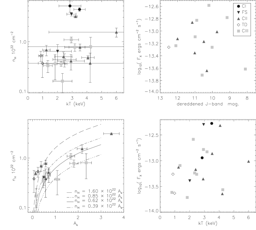
Fig.16(a) shows plasma temperature against the column density of Hydrogen in the intervening gas between us and the hot plasma. The class I and flat spectrum sources show column densities five times greater than the class II and III sources, with one exception. This is not surprising since the class 0/I and flat spectrum sources are surrounded by infalling envelopes. The one exception is a class II object with an unusually high column density, this may be a source where an edge-on disk around the star is occulting the hot plasma. There does appear to be a correlation of plasma temperature with column density: the values of these 26 sources show a Spearman rank coefficient of 0.55. However, the mean values of kT for greater and less than are keV and keV, respectively, indicating that there is no strong dependence. This indicates that the column density is not biasing our determination of the temperature to higher values by selectively absorbing the soft X-ray flux. Soft X-ray photons are more highly absorbed than hard X-ray photons, by up to 90% when (Feigelson et al., 2005). Further more, it shows that there is no significant trend of plasma temperature with evolutionary class.
Fig.16(c) shows the X-ray flux corrected for absorption and for the different classes. Although the class 0/I objects appear slightly more luminous, this may be a bias due to the fact that the class 0/I sources are much more highly absorbed and consequently the weaker class I objects may not have had the 100 counts we require to perform the analysis of the X-ray spectrum. The 8 class II and 9 class III sources have statistically indistinguishable values; the mean values of the class II are keV and and the mean value for the class III sources is keV and . The mean values for the class I are keV and , for the flat spectrum are keV and , and for the transistion disks are keV and . Using the combined class II and class III sample we find only some indication of a weak correlation of kT with X-ray flux, with a Spearman rank coefficient of 0.39. In comparison, Jeffries et al. (2006) find a trend of increasing kT with X-ray in a combined study of several young clusters. Finally, the mean plasma temperatures for the class 0/I and flat spectrum sources are not significantly different than those values for class II and class III sources. Thus, we find no significant dependence of plasma temperature on evolutionary class for the detected X-ray sources.
The X-ray flux of pre-main sequence stars has been found to vary with bolometric luminosity (Feigelson et al., 1993; Casanova et al., 1995). Although we cannot measure the bolometric luminosities, we can examine the X-ray flux as a function of the dereddened J-band magnitude, which is the infrared band least contaminated by infrared excess emission and is thus a good proxy for photospheric emission (Fig.16(b)). We find again that the class II and class III sources appear indistinguishable. In particular, if we limit our analysis to dereddened where we detect 90% of the class II sources in X-rays, we find that the for class II and for class III. A similar lack of dependence is found in NGC 1333 and Ori (Getman et al., 2002; Hernadez et al., 2006). This suggests that the mechanism generating the X-ray flux is similar during the class II and III phases. Getman et al. (2002) find a clear relationship between and J-band magnitude of slope in NGC1333, while Casanova et al. (1995) find a slope of 0.30 in the Ophiuchi cloud. Our results give a slope of , which is consistent with these other young clusters, although there is a large uncecrtainty due to the scatter in our data. In conclusion, we find that there is no clear observational motivation for invoking different mechanisms for generating the X-ray emission in the class I, II and III phases.
The combined X-ray and infrared results can be used to calibrate the relationship between gas column density and the extinction measured in the infrared. We calculated for each star using the method of Gutermuth et al. (2004), which is based on the reddening loci from Meyer et al. (1997) and the extinction law of Flaherty et al. (2007). These values can be compared to the column density of hydrogen atoms, , which is calculated from the inferred absorption of the X-ray emission. Previous measurements of this value lead to an approximately linear fit of (Vuong et al., 2003; Feigelson et al., 2005) for stellar sources, while the value for the diffuse ISM ranges from (Vuong et al., 2003; Gorenstein, 1975). Fig.16(c) plots the hydrogen column density against the calculated exctinction in the K-band. As shown in this plot, the Vuong et al. (2003) relationship agrees with our data for , but diverges from the points with . A similar divergence has also been found in the more deeply embedded stars in the RCW 108 region (Wolk et al., 2007).
Interestingly, the class II sources always show a higher value of for a given . The colors of the class II objects can be affected by both absorption and scattering of the light from the central source by a flared disk; the extent of this effect would be determined, predominantly, by the inclination of the disk and the sizes of grains in the disk (Whitney et al., 2003b). For example, the colors of an edge-on disk system, where the central star is highly obscured by the disk, would be dominated by scattered light. In such a case, the disk absorbs both the infrared and the X-ray emission from the star, but the scattered infrared light reduces the observed reddening of the star and hence the inferred value of . To eliminate the uncertainties in the determination of due to circumstellar material, we fit only the class III objects. The resulting relationship is . Assuming a standard conversion of (Rieke & Lebofsky, 1985), this slope is 2.5 times lower than that derived by previous authors. In comparison, a fit to the class II objects results in . The poor fit and higher slope are further indication that the disks around these objects affect the measurement of , possibly leading to spuriously low values of . We now focus on the slope derived from the class III objects, the possible systematic uncertainties in that slope, and a possible explanation for the low value of the slope.
Systematic underestimation of : If the measurements of were systematically underestimated by a factor of 2.5, then this would lead to the shallower slope observed. However, the determinations of the values appear to be robust. We calculated only for those sources with relatively high S/N ( counts). These values of were found to be consistent using two different models for the plasma. A bias could occur in the determination of when the soft X-ray emission is totally absorbed; however inspection shows that this is not the case here. Furthermore, values of calculated by our software for stars in the Orion COUP survey are within 5% of the values published in Getman et al. (2005); this is further validation of the accuracy of our analysis.
Sytematic overestimation of : The value of is determined by the selective absorption in the near-infrared bands (Gutermuth et al., 2004); this selective absorption was converted to by using an assumed value of . We use the Indebetouw et al. (2005) reddening law where the adopted ratio of . This is equivalent to a near-IR general to selective absorption of . Changes in the reddening law in the molecular cloud could change this ratio. In molecular clouds, Flaherty et al. (2007) report a flattening in the infrared reddening law for compared to the diffuse ISM reddening law measured by Indebetouw et al. (2005); however, they found no significant difference in the reddening law for between the molecular clouds and the diffuse ISM. Alternatively, Nishiyama et al. (2006) report of 1.44, lower than the value in Indebetouw et al. (2005), and they find evidence of variations in this value toward different lines of sight toward the galactic center. If the slope found in our data were wholly due to an overestimation of , then the value of would have to decrease to 0.73, and the value of must change to 2.37. This value of is higher than the values in the literature and would require a steepening of the reddening law between 1 & 2 .
Growth and Coagulation of Dust Grains: The ratio can be affected by increases in the sizes of dust grains; this would simply increase the value of and hence reduce the ratio of . The value of is given by:
where is the column density of dust, is the radius of a dust grain, and is the extinction efficiency (Whittet, 2003). In the limit of , , which would be the case for a standard grain size distribution (Mathis et al., 1977) of ,
where is the refractive index. Thus, there is a strong dependence on the size of the grain, and the value of can be changed simply by growing grains to larger sizes; for example the scattering term in goes as , hence a 25% increase in grain size can increase the scattering efficiency by a factor of 2.5.
Grain growth in molecular clouds may occur through both coagulation and the accretion of grain mantles; these processes would be accelerated in the dense molecular gas found in the Serpens cloud core. For example, Jura (1980) explained changes in the ratio in Ophiuchus through the coagulation of grains. The collision time between grains is (Jura, 1980)
For a and a velocity of 0.1 km s-1 (Jura, 1980), the collision timescale is 30,000 years. Thus it is likely that a dust grain in the Serpens cloud would have had multiple collisions with other grains. Alternatively, the growth can be through the accretion of mantles of volatiles such as H2O, NH3, O2, N2 and CO. The accretion timescale is given by
where s is the specific density of the mantle, is the change in the size of the dust grain due to the mantle, is the sticking coefficient (), is the temperature of the gas, is the density of the molecule forming the mantle, and is the mass of the molecule forming the mantle (Whittet, 2003). Thus the rate of mantle accretion is proportional to the density of the gas; again, the high density of the gas in the Serpens cloud would accelerate the rate of mantle accretion. A detailed calculation of the rate requires consideration of the gas phase abundances of the different possible volatiles, and is beyond the scope of this paper.
Self consistent modeling of the extinction over multiple wavelength bands is needed to study the impact of grain growth on both the relationship between and and the shape of extinction law with which is derived. Further observational work is also needed to confirm our observed slope using a larger number of class III objects from multiple star forming regions. However, this study demonstrates the value of using combined Chandra, near-IR, and Spitzer observations to identify deeply embedded class III objects and search for variations in the extinction law within molecular clouds.
8 Conclusion
We have undertaken an intensive study of the Serpens Cloud Core in the mid-IR with Spitzer and in the near-IR with 2MASS. We have merged these data with Chandra X-ray observations and investigated various X-ray properties of protostars and pre-main sequence stars. These data provide perhaps the most complete census to date of the young stellar objects in one of the nearest embedded clusters to the Sun.
-
•
We identify 138 young stellar objects, after removing contamination. These include 38 protostars (22 class 0/I, 16 Flat Spectrum) and 100 pre-main sequence stars (62 class II, 17 transition disks, and 21 class III). The ratio of protostellar objects (class 0/I and flat spectrum) to pre-main sequence stars (class II, transition disk, and class III) is 38:100 or 29% of the total number of identified members. The ratio of protostars to pre-main sequence stars with disks is 48%. These high numbers indicate that Serpens is unusually rich in protostars. We estimate that as many as 44 class III sources may be missing, implying a total membership of 182.
-
•
We have searched for Spitzer counterparts to 14 (sub)mm sources in the Serpens cluster. Seven are detected as point sources at 3.6-8.0 , a total of 10 have been detected at 24 , and an additional two show nebulosities at . All but one are coincident with 70 emission, although for many of the protostars, the low angular resolution of the 70 data precludes accurate photometry of the sources.
-
•
We find that the spatial distribution of the protostars is distinctly different than the pre-main sequence stars. While the class 0/I sources and most of the flat spectrum sources are concentrated in the central molecular gas filament, the class II, transition disk and class III sources are distributed over a much more extended region. The median projected spacing of the Class 0/I sources is only 5000 AU; these sources are highly clustered. In contrast, the distribution of the remaining classes are statistically indistinguishable from a random distribution.
-
•
The protostars are concentrated in two groups coincident with the two dominant molecular gas clumps, as has been previously reported. The density of protostars in these groups suggest that the volumes of gas from which these protostars accrete may touch or overlap. The spacing is also similar to both the Jean’s length and the radii of critical Bonner Ebert spheres. Based on published ambient gas densities and velocities of the protostars in the northern group, we find that competitive accretion could be occurring in this groups. Furthermore, collisions between protostellar envelopes may be common.
-
•
Of the 138 sources, 60 exhibit detectable X-ray emission. Nine of the detections are associated with class I sources (43% of members in class), a further eight with flat spectrum members (56%). Twenty-one detections have class II counterparts (45%), while only two of the transition disks are detected in X-rays (25%). Twenty class III sources were identified solely by their X-ray emission. There appears to be no evidence of a trend in the detection rate of sources by evolutionary class. The fraction of X-ray detected pre-main sequence stars (i.e. class II, transition disks and class III sources) with disks is 51%.
-
•
We find no evidence for a dependence of the temperature of the X-ray emitting plasma on the evolutionary class, and find no difference in the X-ray luminosity of detected class II and classs III objects. Consequently, there is no evidence that the generation mechanism of the X-ray emission depends on the presence of an infalling envelope or circumstellar disk.
-
•
We find an observed relationship of , which is much shallower than found in other studies. The most likely explanation for this is a change in the near-IR reddening law that would affect the shape and magnitude of the reddening law. Such changes could result from grain coagulation and/or grain growth from the accretion of mantles of volatiles; both such processes may occur relatively quickly due to the high gas (and presumably dust grain) densities in the Serpens cloud core.
This work is based on observations made with the Spitzer Space Telescope (PID 6, PID 174), which is operated by the Jet Propulsion Laboratory, California Institute of Technology under NASA contract 1407. Support for this work was provided by NASA through contract 1256790 issued by JPL/Caltech. Support for the IRAC instrument was provided by NASA through contract 960541 issued by JPL. This publication makes use of data products from the Two Micron All Sky Survey, which is a joint project of the University of Massachusetts and the Infrared Processing and Analysis Center/California Institute of Technology, funded by the National Aeronautics and Space Administration and the National Science Foundation. This research has made use of the NASA/IPAC Infrared Science Archive, which is operated by the Jet Propulsion Laboratory, California Institute of Technology, under contract with the National Aeronautics and Space Administration. E. Winston would like to thank the Irish Research Council for Science, Engineering, and Technology (IRCSET) for funding and support.
References
- Allen et al. (2004) Allen, L., Calvet, N., D’Alessio, P., et al, 2004, ApJSS, 154, 363-366.
- Allen et al. (2006) Allen, L. et al., 2006, Protostars & Planets V.
- Andre et al. (1993) Andre, P., Ward-Thompson, D., & Barsony, M., 1993, ApJ, 406, 122-141.
- Andre et al. (1994) Andre, P., Montmerle, T., 1994, ApJ, 420, 837.
- Armitage et al. (2003) Armitage, P. J., Clarke, C. J. & Francensco, P. 2003, MNRAS,342, 1139.
- Baraffe (1998) Baraffe, I., 1998, A&A, 337, 403,
- Bate & Bonnell (2005) Bate, M. R. & Bonnell, I. A. 2005, MNRAS, 356, 1201
- Blum et al. (2006) Blum, R.D., et al., 2006, ApJ , 132, 2034-2045.
- Bondi & Hoyle (1944) Bondi, H., Hoyle, F., 1944, Mon. Not. R. Astron. Soc., 104, p.273.
- Bonnell & Bate (2005) Bonnell, I. A.& Bate, M. R., 2005, MNRAS, 362, 915.
- Bonnell & Bate (2006) Bonnell, I. A.& Bate, M. R., 2006, MNRAS, 370, 488.
- Bonner (1956) Bonner, W.B., 1956, MNRAS, 116, 351.
- Calvet et al. (2002) Calvet, N., D’Alessio, P., Hartmann, L, Wilner, D, Walsh, A, Sitko, M., 2002, ApJ, 568, 1008.
- Calvet et al. (1994) Calvet, N., Hartmann, L., Kenyon, S.J., Whitney, B.A., 1994, ApJ, 434, 330.
- Carpenter (2000) Carpenter, J.M., 2000, AJ, 120, 3139-3161.
- Casanova et al. (1995) Casanova, S., Montmerle, T., Feigelson, E.D., Andre, P., 1995, ApJ, 439, 752.
- Davis et al. (1999) Davis, C.J., Matthews H.E., Ray T.P., et al, 1999, Mon. Not. R. Astron. Soc 309, 141-152.
- Davis et al. (2000) Davis, C.J., et al., 2000, ApJ, 530, L115-L118.
- Doppman et al. (2005) Doppman, G.W., Greene T.P., Covey K.R., Lada C.J., 2005, ApJ, 130, 1145-1170.
- Ebert (1955) Ebert, R., 1955, Z. Astrophys., 37, 217.
- Eiroa et al. (1992) Eiroa, C., Casali M., 1992, A&A, 262, 468-482.
- Eiroa et al. (2005) Eiroa, C., Torrelles J.M., Curiel S., Djupvik A.A., 2005, ApJ, 130, 643-651.
- Eisenhardt et al. (2004) Eisenhardt, P.R., et al., 2004, ApJS, 154, 48.
- Evans et al. (2003) Evans, N.J. II, et al., 2003, Pub. Astron. Soc. Pacific, 115, 965-980.
- Favata et al. (2003) Favata, et al., 2003, A&A, 403, 187.
- Favata et al. (2005) Favata, et al. , 2005, ApJS, 160, 469.
- Fazio et al. (2004) Fazio, G.G., et al., 2004, ApJS, 154, 10.
- Feigelson et al. (2005) Feigelson, E., Getman, R., et al., 2005, ApJ, 160.
- Feigelson & Montmerle (1999) Feigelson, E. D., Montmerle, T., 1999, ARA&A, 37, 363-408.
- Feigelson et al. (1993) Feigelson, E.D., Casanova, S., Montmerle, T., Guibert, J., 1993, ApJ, 416, 623.
- Feigelson & Kriss (1981) Feigelson, E. D.; Kriss, G. A., 1981, ApJ, 248, L35-L38.
- Flaherty et al. (2007) Flaherty, K.M., et al., 2007, ApJ, submitted.
- Forbrich et a. (2006) Forbrich, J., Preibisch Th., & Menten K.M., 2006, A&A, 446, 155-170.
- Freeman et al. (2001) Freeman, P., Doe, S., Siemiginowska, A., Proc. SPIE Vol. 4477, p. 76-87, Astronomical Data Analysis, Jean-Luc Starck; Fionn D. Murtagh; Eds.
- Gagne et al. (2004) Gagne, M., Skinner, S. L., Daniel, K. J., 2004, ApJ, 613, 393-415.
- Getman et al. (2005) Getman, K. V., et al., 2005, ApJS, 160, 319-352.
- Getman et al. (2002) Getman, K. V., et al., 2002, ApJ, 575, 345-377.
- Giampapa et al. (1996) Giampapa, M.S., et al., 1996, ApJ, 463, 707.
- Giardino et al. (2006) Giardino G., Favata, F., et al., 2007, ApJ (submitted).
- Gordon et al. (2005) Gordon, K. D., et al. 2005, PASP, 117, 503.
- Gorenstein (1975) Gorenstein, P., 1975, ApJ, 198, 95.
- Gutermuth et al. (2005) Gutermuth, R., Megeath, S. T., Pipher, J., Williams, J. P., Allen, L., Myers, P., Raines, S. N., 2005, ApJS, 154, 374.
- Gutermuth et al. (2004) Gutermuth, R., Megeath, S. T., Muzerolle, J., Allen, L., Pipher, J., Myers, P., Fazio, G. G., 2004, ApJS, 154, 374.
- Gutermuth (2005) Gutermuth, R., 2005, PhD Thesis.
- Gutermuth et al. (submitted) Gutermuth, R., et al., 2007, ApJ (submitted).
- Greene et al. (1994) Greene, T.P., Wilking, B.A., Andre, P., Young, E.T., Lada, C.J., 1994, ApJ, 434, 614.
- Haisch et al. (2001) Haisch, K. E. Jr., Lada, E. A. & Lada, C. J. 2001, ApJ, 553, L153.
- Haisch et al. (2006) Haisch, K. E. Jr., Barsony, M., Ressler, M.E., Greene, T.P., 2006, AJ, 132, 2675-2684.
- Hartmann et al. (2005) Hartmann, L., Megeath, S.T., Allen, L.E., Luhman, K., Calvet, N., D’Alessio, P., Franco-Hernandez, R., Fazio, G., 2005, ApJ, 629, 881-896.
- Harvey et al. (2006) Harvey, P., Chapman N., Lai S-P., 2005, ApJ, 644, 30-325.
- Hatchell et al. (submitted) Hatchell, J., arXiv:astro-ph/0612601v1.
- Hayashi et al. (1996) Hayashi, M.R., Hibata, K., Matsumoto. R., 1996, ApJ, 468, L37.
- Hernadez et al. (2006) Hernadez, J., et al., 2006, submitted to ApJ.
- Hogerheijde et al. (1999) Hogerheijde, M., van Dishoeck E., Salverda J., 1999, ApJ, 513, 350-369.
- Hora et al. (2004) Hora, J., et al., Proc. SPIE, 5487, 77.
- Hurt & Barsony (1996) Hurt, R., Barsony M., 1996, ApJ, 460, L45-L48.
- Isobe et al. (2003) Isobe, H., et.al., 2003, PASJ, 55, 967.
- Indebetouw et al. (2005) Indebetouw, R., Mathis, J.S., Bebler, B.L. et al., 2005, ApJ, 619, 931-938.
- Jayawardhana et al. (1999) Jayawardhana, R., Hartmann, L, Fazio, G, Fishter, R. S., Telesco, C. M., & Pina, R. K. 1999, ApJ, 521, L129.
- Jeans (1928) Jeans, J.H., Astronomy & Cosmogony, 1928, The University Press, Cambridge, UK.
- Jeffries et al. (2006) Jeffries, R.D., Evans, P.A., Pye, J.P., Briggs, K.R., 2006, Mon. Not. R. Astron. Soc., 367, 781-800.
- Jijina et al. (1999) Jijina, J., Myers, P.C., Adams, F.C., 1999, ApJ Supplement Series, 125, 161-236.
- Jorgensen et al. (2006) Jorgensen, J., Harvey, P., et al, 2006, ApJ, 645, 1246-1263.
- Jura (1980) Jura, M., 1980, ApJ, 235, 63.
- Kaas et al. (2004) Kaas, A.A., Olofsson G., Bontemps S., et al, 2004, A&A, 421, 623-642.
- Kaas et al. (1999) Kaas, A.A., 1999, AJ, 118, 558-571.
- Kastner et al. (2002) Kastner, J.H., et al., 2002, ApJ, 567, 434.
- Kenyon et al. (1993) Kenyon, S. J., Calvet, N., Hartmann, L., 1993, ApJ, 414, 676.
- Krumholz et al. (2005) Krumholz, M. R., McKee, C. F., & Klein R. I., 2005, Nature, 438, 332.
- Küker & Rüdiger (1999) Küker, M., & Rüdiger, G., 1999, A&A, 346, 922.
- Lada & Wilking (1984) Lada, C.J., Wilking. B.A., 1984, ApJ, 287, 610-621.
- Lada (1987) Lada, C.J., IAU Symp. 115, 1987, Star Forming Regions ed. M Peimbert & J. Jugaku.
- Lada et al. (2006) Lada, C.J., et al., 2006, AJ, 131, 1574.
- Landsman (1989) Landsman, W.B., 1989, Bulletin of Amer. Astron. Soceity, Vol. 21, p784.
- Lin & Papaloizou (1986) Lin, D. N. C., Papaloizou, J., 1986, ApJ, 309, 846-857.
- Luhman (1999) Luhman, K. L. 1999, ApJ, 525, 466.
- Luhman (2001) Luhman, K. L. 2001, ApJ, 560, 287.
- Luhman (2005) Luhman, K.L., 2005, Protostars and Planets V.
- Mathis et al. (1977) Mathis, J.S., Rumpl, W., Nordsiek, K.H., 1977, ApJ, 217, 425.
- McCabe et al. (2006) McCabe, C., Ghez A.M., et al, 2006, ApJ, 636, 932-951.
- Megeath et al. (2004) Megeath, S.T., Gutermuth R.A., Allen L.E., Pipher J.L., Myers P.C., Fazio G.G., 2004, ApJS, 154, 367.
- Megeath et al. (in prep) Megeath, S.T., et al., in prep.
- Meyer et al. (1997) Meyer, M. R.; Calvet, N.; Hillenbrand, L. A., 1997, AJ, 114, 288-300.
- Muzerolle et al. (2004) Muzerolle, J., Megeath, S., Gutermuth, R., Allen, L., Pipher, J., Hartmann, L., et al., 2004, ApJ, 154, 379.
- Nishiyama et al. (2006) Nishiyama, S., et al., 2006, ApJ, 638, 839.
- Olmi & Testi (2002) Olmi, L., Testi L., 2002, A&A, 392, 1053-1068.
- Peterson et al. (submitted) Peterson, D., et al., submitted.
- Porras et al. (2007) Porras, A., et al., 2007, ApJ, 656, 493-504.
- Preibisch (2003) Preibisch, T., 2003, A&A, 410, 951-959.
- Preibisch (2004) Preibisch, T., 2004, A&A, 428, 569-577.
- Preibisch & Feigelson (2005) Preibisch, T., Feigelson, E., 2005, ApJS, Vol. 160.
- Preibisch et al. (2005) Preibisch, T., Kim, , Favata, F., et al., 2005, ApJS, Vol. 160.
- Raymond & Smith (1977) Raymond, J. C., Smith, B. W., 1977, ApJ, 35, 419-439.
- Reach et al. (2005) Reach, W.T., et al., 2005, ASP, 117, 978-990.
- Rebull et al. (2007) Rebull, L.M., et al., 2007, astro-ph/0701711.
- Rieke et al. (2004) Rieke, G., et al., 2004, ApJS, 154, 25-29.
- Rieke & Lebofsky (1985) Rieke, G.H., Lebofsky, M.J., 1985, ApJ, 288, 618-621.
- Romanov et al. (2004) Romanov, M.M., et al., 2004, ApJ, 616, L151.
- Shu (1992) Shu, F. 1992, The Physics of Astrophysics, Vol. II.
- Skrutskie et al. (2006) Skrutskie, M.F., Cutri R.M., Stiening R., et al., 2006, AJ, 131, 1163.
- Slesnick et al. (2004) Slesnick, C. L., Hillenbrand, L. A., Carpenter, J. M., 2004, ApJ, 610, 1045-1063.
- Stern et al. (2005) Stern, D., Eisenhardt, P., Gorjian, V., et al., 2005, ApJ, 631, 163-168.
- Straiz̆ys et al. (2003) Straiz̆ys, V., C̆ernis, K., Bartas̆iūtė, S., 2003, A&A, 405, 585.
- Teixeira et al. (2006) Teixeira, P., Lada, C.J., Young E.T., Marengo M., Muench A., et al., 2006, ApJ, 636, L45-L48.
- Testi et al. (1998) Testi, L., Sargent, A., 1998, ApJ, 508, L91-L94.
- Testi et al. (2000) Testi, L., Sargent, A., Olmi L., Onella J., 2000, ApJ, 540, L53-L56.
- Vuong et al. (2003) Voung, M. H., et al., 2003, A&A, 408, 581-599.
- Werner et al. (2004) Werner, M.W., et al., 2004, ApJS, 154, 1.
- Whitney et al. (2003a) Whitney, B. A., Wood, K., Bjorkman, J. E., Wolff, M. J., 2003, ApJ, 591, 1049-1063.
- Whitney et al. (2003b) Whitney, B. A., Wood, K., Bjorkman, J. E., Cohen, M., 2003, ApJ, 598, 1079-1099.
- Whittet (2003) Whittet, D.C.B., 2003, IOP, Dust in the Galactic Environment, 2nd Ed..
- Williams & Meyers (1999) Williams, J., Meyers P., 1999, ApJ 518, L37-L40.
- Williams & Meyers (2000) Williams, J., Meyers P., 2000, ApJ, 537, 891-903.
- Wolk et al. (2006) Wolk, S. J., Spitzbart, B. D., Bourke, T. L., Alves, J., 2006, AJ, 132, 1100-1125.
- Wolk et al. (2007) Wolk, S. J., Bourke, T. L., et al., 2007, in prep.
- Young et al. (2006) Young, E.T., Teixeira, P.S., et al. , 2006, ApJ, 642, 972-978.
| IR-excess | X-ray Detected | Extremely Red | Total | |
|---|---|---|---|---|
| Identified | 200 | 67 | 3 | 229 |
| Contam. | 87 | 7 | 1 | 91 |
| YSOs | 113 | 60 | 2 | 138 |
| Class | IR-field | IRX-field | X-ray Detections |
|---|---|---|---|
| 0/I | 22 | 22 | 9 ( 43%) |
| Flat | 16 | 15 | 8 ( 53%) |
| II | 62 | 44 | 20 ( 46%) |
| Trans. | 17 | 8 | 2 ( 25%) |
| III | 21 | 21 | 21 |
| I | Flat | II | Trans. | III | |
|---|---|---|---|---|---|
| Random | 0.05 | 0.13 | 0.67 | 0.21 | |
| I | |||||
| Flat | 0.45 | 0.28 | 0.73 | ||
| II | 0.45 | 0.016 | 0.60 | ||
| Trans. | 0.28 | 0.016 | 0.35 |
| Spitzer ID | RA (2000) | Dec (2000) | EC aaIdentifiers from Eiroa et al. (1992). | Kaas bbIdentifiers from Kaas et al. (2004). | Class 0 ccIdentifiers from Testi et al. (1998); Williams & Meyers (1999); Davis et al. (1999). | Chandra ID | GFG ID ddIdentifiers from Giardino et al. (2006). |
|---|---|---|---|---|---|---|---|
| 1 | 18:30:02.09 | 1:13:58.81 | CK7 | ||||
| 2 | 18:29:57.83 | 1:12:51.62 | EC95 | Kaas317/345 | 72 | 53 | |
| 3 | 18:29:59.57 | 1:11:58.80 | Kaas330 | 25 | 60 | ||
| 4 | 18:29:58.76 | 1:14:26.47 | EC103 | Kaas326 | 23 | ||
| 5 | 18:29:47.01 | 1:16:26.82 | EC27 | Kaas237 | |||
| 6 | 18:29:49.24 | 1:16:31.74 | Kaas249 | ||||
| 7 | 18:29:49.58 | 1:17:05.92 | EC76 | Kaas254 | S68Nb | 17 | 28 |
| 8 | 18:29:57.59 | 1:13:00.44 | SVS4-10 | Kaas312 | 12 | 46 | |
| 9 | 18:29:56.88 | 1:14:46.62 | CK3 | Kaas307 | 67 | 43 | |
| 10 | 18:30:02.73 | 1:12:28.14 | EC129 | Kaas347 | PS2 | ||
| 11 | 18:29:49.11 | 1:16:19.97 | SN68d | ||||
| 12 | 18:29:57.64 | 1:13:04.54 | |||||
| 17 | 18:30:00.68 | 1:13:01.23 | |||||
| 18 | 18:29:59.92 | 1:13:11.58 | Kaas331 | ||||
| 19 | 18:29:59.61 | 1:14:12.33 | 78 | 61 | |||
| 20 | 18:29:52.85 | 1:14:56.08 | Kaas276 | 33 | |||
| 21 | 18:29:52.20 | 1:15:47.59 | Kaas270 | SMM10 | |||
| 22 | 18:29:52.20 | 1:15:59.02 | 20 | 32 | |||
| 23 | 18:29:48.09 | 1:16:44.98 | Kaas241 | SMM9/S68N | |||
| 24 | 18:29:51.14 | 1:16:40.49 | Kaas265 | SMM5 | 18 | 30 | |
| 27 | 18:29:58.18 | 1:15:21.91 | CK4 | Kaas321 | 74 | 55 | |
| 28 | 18:30:00.20 | 1:14:03.56 | 79 | 62 | |||
| 30 | 18:30:01.09 | 1:13:24.44 | EC121 | Kaas341 | 81 | 66 | |
| 31 | 18:30:01.53 | 1:15:14.93 | EC123 | SMM8 | |||
| 32 | 18:29:18.85 | 1:14:16.94 | |||||
| 33 | 18:30:23.43 | 1:05:04.84 | |||||
| 34 | 18:29:53.84 | 1:12:47.40 | |||||
| 35 | 18:29:57.72 | 1:14:06.06 | SVS20 | Kaas314 | SMM6 | 70 | 48 |
| 36 | 18:29:31.97 | 1:18:42.66 | Kaas159 | 9 | 9 | ||
| 37 | 18:29:57.82 | 1:12:37.97 | EC94 | Kaas318 | 22 | 52 | |
| 38 | 18:29:55.68 | 1:14:31.34 | CK9 | Kaas298 | 63 | 37 | |
| 39 | 18:29:54.07 | 1:07:11.10 | Kaas287 | ||||
| 40 | 18:30:18.17 | 1:14:16.89 | 44 | 83 | |||
| 44 | 18:29:59.38 | 1:10:40.92 | |||||
| 45 | 18:29:59.02 | 1:12:24.92 | Kaas327 | ||||
| 47 | 18:30:02.48 | 1:12:43.44 | |||||
| 48 | 18:29:49.70 | 1:14:56.71 | EC40 | Kaas253 | |||
| 53 | 18:29:14.32 | 1:07:30.14 | |||||
| 54 | 18:30:05.01 | 1:12:35.99 | |||||
| 55 | 18:30:22.83 | 1:16:21.34 | |||||
| 56 | 18:29:55.56 | 1:08:34.34 | |||||
| 57 | 18:29:21.08 | 1:24:06.66 | |||||
| 58 | 18:30:22.74 | 1:13:23.58 | |||||
| 59 | 18:29:59.22 | 1:14:07.82 | CK8 | Kaas328 | 77 | 59 | |
| 60 | 18:30:04.09 | 1:06:55.86 | |||||
| 61 | 18:29:56.66 | 1:12:39.17 | EC80 | Kaas306 | 21 | 42 | |
| 62 | 18:29:55.19 | 1:13:22.43 | EC73 | Kaas294 | |||
| 64 | 18:29:38.18 | 1:09:17.53 | |||||
| 65 | 18:29:43.92 | 1:07:20.99 | Kaas219 | ||||
| 66 | 18:29:51.43 | 1:09:32.94 | |||||
| 67 | 18:30:09.22 | 1:17:52.66 | |||||
| 68 | 18:29:47.19 | 1:07:16.02 | |||||
| 69 | 18:29:53.83 | 1:13:30.80 | EC68 | Kaas285 | |||
| 70 | 18:29:57.81 | 1:12:28.17 | EC91 | Kaas320 | |||
| 71 | 18:29:44.28 | 1:04:53.50 | Kaas221 | ||||
| 72 | 18:29:04.26 | 1:18:39.08 | |||||
| 73 | 18:30:07.70 | 1:12:04.49 | Kaas366 | 86 | 75 | ||
| 74 | 18:30:13.28 | 1:02:48.93 | |||||
| 75 | 18:29:32.24 | 1:12:39.94 | |||||
| 76 | 18:30:16.97 | 1:13:07.47 | |||||
| 77 | 18:30:00.89 | 1:22:03.59 | |||||
| 78 | 18:30:03.41 | 1:16:19.45 | EC135 | Kaas348 | 84 | 69 | |
| 79 | 18:29:46.28 | 1:10:25.33 | |||||
| 80 | 18:29:56.53 | 1:12:59.53 | SVS4-2 | Kaas304 | 66 | 40 | |
| 81 | 18:29:53.59 | 1:17:01.91 | EC67 | Kaas283 | 60 | 34 | |
| 82 | 18:29:33.37 | 1:08:24.42 | Kaas173 | ||||
| 83 | 18:29:57.80 | 1:15:31.89 | CK13 | Kaas319 | 71 | 50 | |
| 84 | 18:30:06.08 | 1:06:17.11 | Kaas357 | 42 | 73 | ||
| 85 | 18:29:56.94 | 1:12:47.88 | EC84 | Kaas309 | 68 | 44 | |
| 86 | 18:29:53.16 | 1:12:27.78 | |||||
| 87 | 18:29:54.50 | 1:14:47.11 | EC70 | Kaas291 | 61 | 35 | |
| 88 | 18:30:41.16 | 1:13:15.94 | |||||
| 89 | 18:30:14.42 | 1:04:06.44 | |||||
| 90 | 18:30:44.52 | 1:23:30.19 | |||||
| 91 | 18:29:35.18 | 1:13:10.95 | |||||
| 92 | 18:30:01.66 | 1:04:42.96 | |||||
| 93 | 18:29:42.15 | 1:20:20.93 | Kaas216 | 47 | |||
| 94 | 18:29:39.87 | 1:17:56.02 | Kaas202 | 57 | 18 | ||
| 95 | 18:29:51.18 | 1:13:19.71 | EC51 | Kaas266 | 49 | 31 | |
| 96 | 18:29:53.09 | 1:06:17.85 | |||||
| 97 | 18:29:05.82 | 1:13:22.94 | |||||
| 98 | 18:30:04.89 | 1:14:39.48 | 85 | 71 | |||
| 99 | 18:29:53.54 | 1:13:05.34 | |||||
| 100 | 18:29:44.53 | 1:13:11.59 | EC11 | Kaas224 | 59 | 23 | |
| 101 | 18:30:11.09 | 1:12:37.93 | Kaas393 | 87 | 79 | ||
| 102 | 18:30:27.67 | 1:22:35.02 | |||||
| 103 | 18:29:41.44 | 1:07:38.15 | Kaas207 | ||||
| 104 | 18:29:20.41 | 1:21:03.78 | |||||
| 105 | 18:29:57.89 | 1:12:46.42 | EC98 | Kaas322 | 73 | 54 | |
| 106 | 18:29:48.77 | 1:13:42.12 | EC33 | Kaas242 | |||
| 109 | 18:30:02.31 | 1:08:08.82 | |||||
| 110 | 18:30:00.31 | 1:09:44.59 | 13 | 63 | |||
| 112 | 18:29:56.28 | 1:13:21.14 | |||||
| 114 | 18:29:49.69 | 1:15:28.85 | Kaas258 | ||||
| 115 | 18:29:38.59 | 1:18:01.39 | |||||
| 118 | 18:30:01.79 | 1:18:59.84 | |||||
| 119 | 18:29:29.80 | 1:21:57.38 | 5 | 6 | |||
| 122 | 18:29:13.01 | 1:07:00.64 | |||||
| 124 | 18:29:08.17 | 1:05:44.68 | |||||
| 127 | 18:29:37.67 | 1:11:30.01 | |||||
| 128 | 18:30:23.12 | 1:20:09.65 | 46 | 85 | |||
| 134 | 18:29:37.58 | 1:11:17.55 | |||||
| 136 | 18:29:16.36 | 1:08:22.13 | |||||
| 140 | 18:30:37.33 | 1:16:09.02 | |||||
| 143 | 18:30:53.70 | 1:11:20.64 | |||||
| 156 | 18:30:00.07 | 1:03:05.81 | |||||
| 157 | 18:30:22.39 | 1:20:44.12 | 45 | 84 | |||
| 158 | 18:30:00.60 | 1:15:20.21 | |||||
| 161 | 18:30:17.29 | 1:21:32.83 | |||||
| 165 | 18:29:58.43 | 1:12:50.35 | 75 | ||||
| 166 | 18:30:13.96 | 1:08:51.47 | Kaas407 | ||||
| 170 | 18:30:09.43 | 1:02:47.06 | Kaas379 | ||||
| 174 | 18:30:03.58 | 1:16:41.04 | |||||
| 176 | 18:29:41.52 | 1:10:04.52 | |||||
| 180 | 18:29:47.64 | 1:04:22.28 | |||||
| 181 | 18:30:19.60 | 1:05:34.31 | |||||
| 187 | 18:30:16.80 | 1:19:17.13 | |||||
| 189 | 18:30:03.01 | 1:19:49.71 | 83 | ||||
| 190 | 18:29:57.39 | 1:14:50.47 | 88 | 45 | |||
| 192 | 18:29:57.65 | 1:10:53.56 | 69 | 47 | |||
| 193 | 18:29:57.55 | 1:10:47.01 | 50 | ||||
| 195 | 18:30:01.24 | 1:15:03.73 | 82 | 67 | |||
| 196 | 18:29:59.11 | 1:11:20.09 | 76 | 58 | |||
| 198 | 18:29:59.05 | 1:11:13.82 | 24 | 57 | |||
| 199 | 18:29:47.21 | 1:22:34.69 | 40 | 27 | |||
| 201 | 18:29:55.34 | 1:10:34.31 | 62 | 36 | |||
| 203 | 18:30:05.50 | 1:14:24.87 | 51 | 72 | |||
| 204 | 18:29:56.33 | 1:12:18.04 | 65 | 39 | |||
| 205 | 18:29:56.17 | 1:10:57.66 | 64 | 38 | |||
| 209 | 18:29:50.53 | 1:08:58.22 | 41 | 29 | |||
| 215 | 18:29:42.32 | 1:12:01.99 | 58 | 21 | |||
| 216 | 18:30:00.64 | 1:13:40.38 | Serpens13 | Kaas338 | 80 | 65 | |
| 218 | 18:29:49.47 | 1:12:04.29 | 48 | ||||
| 220 | 18:30:24.44 | 1:19:50.66 | 36 | ||||
| 221 | 18:29:22.70 | 1:10:33.09 | 37 | 2 | |||
| 224 | 18:29:31.64 | 1:15:05.59 | 54 | ||||
| 225 | 18:29:33.06 | 1:17:16.68 | 56 | 11 |
| ID | J | H | K | 3.6 | 4.5 | 5.8 | 8.0 | 24.0 | Class | CID aaChandra X-ray Idenifier number. | bbSlope of SED calculated from available IRAC data points. Note slopes of FS objects fall between -0.30.3 when 24 point is included. | AK ccThis source was saturated at 24 , the photometry was fit using the PSF wings as described in text. |
|---|---|---|---|---|---|---|---|---|---|---|---|---|
| 1 | 16.044 | 14.9210.118 | 13.3890.046 | 10.6510.003 | 9.8060.002 | 9.0810.003 | 8.2070.002 | 4.0300.004 | 0/1 | -0.06 | ||
| 2 | 15.7520.093 | 12.4550.045 | 10.5180.029 | 8.6460.004 | 7.6800.003 | 6.8740.004 | 5.6390.004 | 1.0990.013 | 0/1 | 72 | 0.56 | |
| 3 | 17.913 | 17.371 | 14.6490.099 | 8.9590.003 | 7.2630.002 | 6.1950.002 | 5.3090.001 | 1.5040.006 | 0/1 | 25 | 1.27 | |
| 4 | 15.185 | 14.0250.069 | 11.8430.042 | 9.4850.004 | 8.3830.005 | 7.3320.005 | 6.6190.005 | 2.4710.021 | 0/1 | 23 | 0.46 | |
| 5 | 17.731 | 15.836 | 13.4030.041 | 11.0410.004 | 10.2180.005 | 9.6140.007 | 8.9100.004 | 5.4630.022 | 0/1 | -0.44 | ||
| 6 | 18.248 | 17.326 | 13.4460.04 | 10.7420.004 | 9.3220.004 | 8.2550.003 | 7.0510.006 | 1.6650.022 | 0/1 | 1.35 | ||
| 7 | 16.889 | 15.6580.145 | 12.670.036 | 9.6210.002 | 8.2820.003 | 7.3020.002 | 6.4470.002 | 2.7410.009 | 0/1 | 17 | 0.76 | |
| 8 | 16.454 | 14.104 | 13.0550.085 | 9.1880.007 | 7.6650.004 | 6.7470.004 | 5.9770.007 | 1.4310.014 | 0/1 | 12 | 0.77 | |
| 9 | 12.0460.045 | 10.7850.057 | 9.2980.034 | 6.8220.002 | 6.0790.002 | 5.5410.001 | 4.2280.001 | 0.5740.008 | 0/1 | 67 | 0.06 | |
| 10 | 15.2040.061 | 11.920.033 | 9.9170.023 | 7.7160.002 | 6.7890.002 | 6.0440.002 | 5.1990.001 | 1.2670.004 | 0/1 | 0.01 | ||
| 11 | 18.253 | 17.301 | 14.9250.200 | 11.0320.005 | 8.6560.004 | 6.8970.004 | 5.1780.002 | -0.030.1 ccThis source was saturated at 24 , the photometry was fit using the PSF wings as described in text. | 0/1 | 2.21 | ||
| 12 | 16.0460.113 | 13.7650.055 | 12.0230.052 | 10.1370.008 | 9.2170.006 | 0/1 | 0.74 | |||||
| 17 | 14.1290.059 | 12.4600.029 | 11.4620.029 | 10.3540.023 | 0/1 | 1.39 | ||||||
| 18 | 12.6290.019 | 9.5130.003 | 7.6720.002 | 6.2620.002 | 0.9870.008 | 0/1 | 4.35 | |||||
| 19 | 12.3410.035 | 11.4060.031 | 10.3130.044 | 5.2420.037 | 0/1 | 78 | 1.03 | |||||
| 20 | 11.3860.005 | 9.4330.003 | 8.1140.002 | 6.9790.003 | 1.8760.006 | 0/1 | 2.16 | |||||
| 21 | 11.5340.005 | 9.6170.003 | 8.7240.003 | 7.9580.002 | 1.7290.009 | 0/1 | 1.12 | |||||
| 22 | 15.7810.081 | 12.6970.012 | 11.0270.009 | 10.2350.012 | 0/1 | 20 | 3.40 | |||||
| 23 | 12.9690.006 | 11.1180.004 | 10.0390.005 | 9.0690.005 | 3.5070.036 | 0/1 | 1.54 | |||||
| 24 | 10.0110.002 | 8.7010.005 | 7.4040.002 | 6.3560.002 | 1.8130.007 | 0/1 | 18 | 1.38 | ||||
| 27 | 13.0720.029 | 11.1880.028 | 9.8590.022 | 8.2780.002 | 7.6540.002 | 7.1810.002 | 6.4050.001 | 2.7740.011 | FS | 74 | -0.74 | |
| 28 | 15.7060.086 | 13.9120.033 | 12.8210.018 | 11.3200.006 | 10.7490.004 | 10.0940.024 | 9.0610.021 | 5.5770.034 | FS | 79 | -0.26 | |
| 30 | 17.925 | 15.3670.12 | 13.220.033 | 11.1170.003 | 10.3140.003 | 9.8620.006 | 9.2440.006 | 4.90990.103 | FS | 81 | -0.77 | |
| 31 | 11.5440.083 | 6.3210.050 | 0/1 | |||||||||
| 32 | 16.6740.16 | 15.4530.135 | 14.8480.148 | 13.7200.013 | 12.3490.011 | 11.4670.017 | 10.8980.024 | 7.5270.022 | FS | 0.34 | ||
| 33 | 13.4030.03 | 12.4340.035 | 11.7790.023 | 10.8450.002 | 10.2870.002 | 9.8920.005 | 9.1130.003 | 5.2680.005 | FS | -0.91 | ||
| 34 | 18.32 | 17.294 | 15.1150.166 | 14.0530.010 | 13.5360.012 | 13.0130.031 | 12.1360.029 | 8.9540.061 | FS | -0.67 | ||
| 35 | 12.2220.026 | 9.2420.036 | 7.0510.024 | 5.2310.002 ddPhotometry at this wavelength is saturated. | 4.3860.002 ddPhotometry at this wavelength is saturated. | 3.4260.001 | 2.5910.001 ddPhotometry at this wavelength is saturated. | -0.330.1 ccThis source was saturated at 24 , the photometry was fit using the PSF wings as described in text. | FS | 70 | 0.21 | |
| 36 | 11.6310.024 | 9.8030.032 | 8.5840.021 | 6.9680.001 | 5.9210.002 | 5.0450.001 | 3.9170.001 | 0.510.1 ccThis source was saturated at 24 , the photometry was fit using the PSF wings as described in text. | FS | 9 | 0.62 | |
| 37 | 17.197 | 14.4120.061 | 11.6640.028 | 9.7090.003 | 8.7930.004 | 8.2260.005 | 7.5680.005 | FS | 22 | -0.45 | ||
| 38 | 15.3370.05 | 12.4690.026 | 10.6530.018 | 9.2810.003 | 8.2680.002 | 7.4420.002 | 6.7320.003 | 3.7080.016 | FS | 63 | 0.06 | |
| 39 | 15.9810.118 | 14.3560.049 | 13.510.047 | 11.8080.004 | 11.3580.004 | 10.9640.008 | 10.2260.009 | 7.0570.007 | FS | -1.07 | ||
| 40 | 13.3070.026 | 11.7730.032 | 10.8950.02 | 10.4760.002 | 9.9310.002 | 9.2780.003 | 8.2750.004 | 4.3930.007 | FS | 44 | -0.32 | |
| 44 | 14.1390.010 | 12.0520.005 | 10.9310.007 | 10.1820.007 | 6.8240.014 | FS | 1.59 | |||||
| 45 | 12.7740.007 | 11.8010.006 | 11.0670.012 | 10.1760.011 | 5.8990.012 | FS | 0.09 | |||||
| 47 | 13.5430.011 | 12.6690.013 | 11.7070.046 | 11.1530.063 | FS | -0.06 | ||||||
| 48 | 10.7880.003 | 9.1930.003 | 8.1710.002 | 7.3930.002 | 4.2250.020 | FS | 0.99 | |||||
| 53 | 14.6090.036 | 13.6580.037 | 13.1470.032 | 12.4780.005 | 12.1620.005 | 11.9180.015 | 11.3290.013 | 8.7180.041 | 2 | -1.58 | 0.21 | |
| 54 | 15.9490.11 | 14.6960.096 | 13.7320.051 | 12.7010.005 | 12.2760.003 | 11.8650.019 | 11.2240.025 | 2 | -1.18 | 0.28 | ||
| 55 | 15.6190.084 | 14.4260.068 | 13.5890.057 | 13.0130.012 | 12.7480.030 | 12.4770.057 | 2 | -1.85 | 0.29 | |||
| 56 | 14.229 | 14.7680.098 | 14.3190.107 | 13.2480.014 | 12.7550.011 | 2 | -0.93 | |||||
| 57 | 16.2770.132 | 15.3530.114 | 14.7640.115 | 13.9470.031 | 2 | 0.09 | ||||||
| 58 | 16.0210.094 | 15.0350.111 | 14.5470.091 | 13.7330.017 | 13.3110.015 | 12.5920.168 | 2 | -0.67 | 0.29 | |||
| 59 | 11.750.025 | 10.3680.03 | 9.5050.02 | 8.1030.003 | 7.4480.004 | 6.8880.009 | 6.1530.009 | 4.0300.015 | 2 | 77 | -0.64 | 0.57 |
| 60 | 16.7730.203 | 14.8760.077 | 14.1680.067 | 13.3580.008 | 13.0660.009 | 12.6600.023 | 12.1120.038 | 8.2010.016 | 2 | -1.43 | 0.45 | |
| 61 | 18.127 | 16.539 | 14.0560.056 | 10.6830.004 | 9.2690.003 | 8.7610.005 | 8.4280.005 | 5.5010.025 | 2 | 21 | -0.39 | |
| 62 | 16.0350.108 | 13.4690.036 | 12.0270.025 | 10.8300.004 | 10.2660.004 | 9.8930.006 | 9.0760.004 | 4.9270.008 | 2 | -0.90 | 1.92 | |
| 64 | 15.9030.106 | 14.7510.073 | 14.5150.116 | 13.0690.022 | 13.0690.023 | 2 | -2.86 eeSlope & classification uncertain due to lack of photometry in all Spitzer bands. The IR-excess may be due to a mismatch between the 2MASS & IRAC photometry. | 0.58 | ||||
| 65 | 13.8960.028 | 12.450.031 | 11.5960.024 | 10.5090.002 | 10.0650.002 | 9.7370.004 | 9.3290.004 | 6.9610.009 | 2 | -1.53 | 0.68 | |
| 66 | 15.6660.073 | 14.9630.092 | 13.202 | 13.6920.014 | 13.4020.017 | 12.8970.043 | 12.6970.071 | 2 | -1.68 | |||
| 67 | 15.4190.065 | 13.9740.046 | 12.9530.032 | 11.3630.003 | 10.8780.003 | 10.5030.006 | 9.9480.005 | 7.1070.012 | 2 | -1.27 | 0.53 | |
| 68 | 15.9120.09 | 14.8180.068 | 14.4270.086 | 13.8150.009 | 13.3860.009 | 13.0860.038 | 12.1680.027 | 2 | -1.03 | 0.52 | ||
| 69 | 16.4530.146 | 14.2860.048 | 13.010.035 | 11.8970.005 | 11.5310.005 | 10.8890.009 | 10.2690.011 | 7.2660.036 | 2 | -0.94 | 1.44 | |
| 70 | 18.165 | 15.8230.176 | 12.9690.033 | 10.8560.004 | 9.9080.003 | 9.4660.011 | 8.9670.014 | 6.0450.023 | 2 | -0.77 | 3.51 | |
| 71 | 8.5180.019 | 6.5480.038 | 5.3820.02 | 4.2670.002 | 3.4480.001 | -0.2410.009 | 2 | 0.18 | 1.23 | |||
| 72 | 16.6760.185 | 15.9880.192 | 15.4890.216 | 14.4660.019 | 14.3700.025 | 2 | 3 | -2.49 eeSlope & classification uncertain due to lack of photometry in all Spitzer bands. The IR-excess may be due to a mismatch between the 2MASS & IRAC photometry. | ||||
| 73 | 12.2480.023 | 10.8380.032 | 10.0680.023 | 8.9440.003 | 8.4750.003 | 8.0720.002 | 7.3010.001 | 4.3360.003 | 2 | 86 | -1.01 | 0.70 |
| 74 | 13.7190.029 | 12.7690.033 | 12.3510.025 | 11.8360.004 | 11.6350.004 | 11.4200.012 | 10.7860.017 | 7.5820.023 | 2 | -1.69 | 0.29 | |
| 75 | 16.2960.113 | 15.7260.156 | 14.8560.122 | 14.6580.0168 | 14.5790.022 | 14.2660.079 | 2 | -2.13 eeSlope & classification uncertain due to lack of photometry in all Spitzer bands. The IR-excess may be due to a mismatch between the 2MASS & IRAC photometry. | ||||
| 76 | 16.4790.147 | 15.1760.137 | 14.2410.086 | 13.3740.009 | 12.9270.007 | 12.6060.022 | 12.0170.033 | 8.3140.058 | 2 | -1.34 | 0.38 | |
| 77 | 15.860.093 | 15.0840.11 | 14.5150.10 | 13.9650.026 | 13.7920.028 | 13.3610.127 | 2 | -1.72 | ||||
| 78 | 12.2830.03 | 11.0530.035 | 10.3820.026 | 9.7090.002 | 9.3170.002 | 8.9490.003 | 7.7490.002 | 4.4850.004 | 2 | 84 | -0.65 | 0.51 |
| 79 | 13.210 0.026 | 12.3090.028 | 11.9180.023 | 11.2450.002 | 10.9230.003 | 10.5940.006 | 10.0380.005 | 7.8480.008 | 2 | -1.49 | 0.23 | |
| 80 | 15.0130.056 | 12.8050.035 | 11.5220.025 | 10.1960.004 | 9.6370.005 | 9.0880.007 | 8.4120.008 | 5.1360.037 | 2 | 66 | -0.82 | 1.48 |
| 81 | 12.6050.022 | 11.2390.031 | 10.4110.021 | 9.5770.002 | 9.2480.002 | 8.9230.003 | 8.3240.002 | 5.9270.013 | 2 | 60 | -1.45 | 0.58 |
| 82 | 9.7930.026 | 9.3690.027 | 9.2110.023 | 8.8410.003 | 8.5210.004 | 8.0010.002 | 6.8210.003 | 4.0970.004 | 2 | -0.54 | ||
| 83 | 16.2060.138 | 12.7920.036 | 10.8050.022 | 9.2090.003 | 8.5740.004 | 8.2790.003 | 7.7530.004 | 4.6980.024 | 2 | 71 | -1.26 | 2.76 |
| 84 | 12.940.026 | 11.8330.032 | 11.230.022 | 10.4990.002 | 10.1250.002 | 9.7750.004 | 8.9030.003 | 5.7910.003 | 2 | 42 | -1.06 | 0.38 |
| 85 | 15.1680.051 | 12.4730.035 | 11.0870.025 | 9.9190.004 | 9.5130.006 | 9.0290.006 | 8.5910.017 | 2 | 68 | -1.32 | 2.17 | |
| 86 | 16.8340.002 | 15.6820.141 | 14.4530.094 | 13.5270.008 | 13.1190.008 | 12.6420.021 | 11.7770.017 | 2 | -0.86 | 1.33 | ||
| 87 | 14.1740.041 | 13.3320.042 | 12.8 0.035 | 12.3000.008 | 12.1320.009 | 11.9370.028 | 11.8470.053 | 3 | 61 | -2.35 | 0.02 | |
| 88 | 14.5040.038 | 13.7280.045 | 13.2440.034 | 12.4950.005 | 12.1090.005 | 11.6450.012 | 10.8860.013 | 7.7260.048 | 2 | -1.02 | ||
| 89 | 15.2460.065 | 14.3120.056 | 13.9210.065 | 12.9620.007 | 12.4840.006 | 12.0740.017 | 11.3770.015 | 8.8680.016 | 2 | -1.07 | 0.29 | |
| 90 | 14.481 | 14.690.083 | 14.5010.092 | 13.8880.016 | 13.5160.013 | 2 | -1.41 | |||||
| 91 | 15.4840.07 | 14.4510.08 | 13.690.068 | 12.8730.006 | 12.5790.006 | 12.2420.017 | 11.7830.016 | 2 | -1.62 | 0.11 | ||
| 92 | 16.0690.115 | 14.1870.052 | 13.0970.034 | 12.0470.005 | 11.4330.004 | 11.0620.009 | 10.1980.014 | 6.8470.025 | 2 | -0.80 | 1.16 | |
| 93 | 13.2860.027 | 12.5170.035 | 12.0420.03 | 11.5220.005 | 11.1950.003 | 10.6470.006 | 9.3380.003 | 6.3510.003 | 2 | 47 | -0.35 | |
| 94 | 14.4710.034 | 12.830.032 | 11.9370.026 | 10.9830.003 | 10.5730.003 | 10.1980.006 | 9.3880.005 | 6.2940.006 | 2 | 57 | -1.06 | 0.95 |
| 95 | 16.4820.141 | 14.5120.056 | 13.6010.047 | 12.7590.006 | 12.4380.007 | 12.1290.019 | 11.4450.021 | 8.5580.022 | 2 | 49 | -1.38 | 1.44 |
| 96 | 14.3830.035 | 13.0520.032 | 12.5610.028 | 11.4290.003 | 11.2760.003 | 10.9130.007 | 10.2360.006 | 7.4930.011 | 2 | -1.48 | 0.77 | |
| 97 | 16.3410.129 | 15.7960.154 | 14.814 | 14.4820.015 | 14.3820.022 | 2 | -2.47 eeSlope & classification uncertain due to lack of photometry in all Spitzer bands. The IR-excess may be due to a mismatch between the 2MASS & IRAC photometry. | |||||
| 98 | 13.6630.029 | 12.7160.032 | 12.2410.026 | 11.7340.004 | 11.2810.004 | 10.9090.008 | 10.2600.008 | 8.1160.025 | 2 | 85 | -1.20 | 0.24 |
| 99 | 14.890.041 | 14.1270.036 | 13.7420.057 | 13.0130.008 | 12.7080.008 | 12.5180.022 | 12.1050.027 | 2 | -1.86 | 0.03 | ||
| 100 | 13.2290.024 | 12.2170.035 | 11.7650.028 | 11.2620.003 | 11.0330.003 | 10.6690.007 | 9.8370.006 | 6.9620.004 | 2 | 59 | -0.23 | 0.36 |
| 101 | 13.258 | 12.4810.037 | 11.9560.026 | 11.1470.003 | 10.8930.003 | 10.2380.006 | 9.3470.005 | 6.4250.005 | 2 | 87 | -0.74 | 0.14 |
| 102 | 15.9480.119 | 15.3150.129 | 14.4820.093 | 14.2120.017 | 14.1610.018 | 13.8190.089 | 2 | -2.12 eeSlope & classification uncertain due to lack of photometry in all Spitzer bands. The IR-excess may be due to a mismatch between the 2MASS & IRAC photometry. | ||||
| 103 | 11.6030.022 | 10.3860.028 | 9.6440.019 | 8.7280.002 | 8.3990.002 | 8.0730.002 | 7.2440.001 | 4.1690.005 | 2 | -1.18 | 0.42 | |
| 104 | 12.8330.033 | 11.2500.041 | 10.3250.028 | 9.4490.002 | 9.1490.002 | 8.8990.003 | 8.5170.003 | 5.9840.013 | 2 | -1.82 | 0.83 | |
| 105 | 16.553 | 12.5200.042 | 9.9690.034 | 8.4490.003 | 7.7140.003 | 7.0530.004 | 6.3530.006 | 2 | 73 | -0.46 | 3.45 | |
| 106 | 17.230 | 15.2880.106 | 13.4510.041 | 12.0750.004 | 11.3680.003 | 10.9540.008 | 10.3090.008 | 7.4910.015 | 2 | -0.89 | 1.84 | |
| 109 | 13.2470.006 | 12.1520.005 | 11.3810.011 | 10.6770.015 | 8.6780.033 | 2 | 0.06 | |||||
| 110 | 10.5050.002 | 8.9890.003 | 7.9710.002 | 7.2360.002 | 4.8170.003 | 2 | 13 | 0.86 | ||||
| 112 | 14.9650.131 | 13.7800.068 | 13.0380.111 | 12.5310.091 | 2 | -0.11 | ||||||
| 114 | 12.8040.019 | 11.7250.029 | 11.1240.039 | 10.4320.049 | 2 | -0.21 | ||||||
| 115 | 14.6430.018 | 14.2810.025 | 14.1230.071 | 13.6680.157 | 2 | -1.81 | ||||||
| 118 | 14.600.027 | 14.3370.025 | 14.0360.073 | 13.5360.101 | 2 | -1.65 | ||||||
| 119 | 14.2090.016 | 13.6270.050 | 13.0210.045 | 2 | 5 | -1.09 | ||||||
| 122 | 8.7510.02 | 7.2740.047 | 6.5950.02 | 6.1820.001 | 6.2150.002 | 5.9710.002 | 5.8190.002 | 4.9120.004 | TD | -2.42 | 0.89 | |
| 124 | 10.6590.022 | 10.2410.031 | 10.0710.019 | 9.8790.002 | 9.9520.002 | 9.8650.005 | 9.6780.006 | 7.5070.008 | TD | -2.63 | ||
| 127 | 11.4560.022 | 9.5860.027 | 8.8250.024 | 8.1660.002 | 8.1790.003 | 7.9310.002 | 7.7220.002 | 6.2140.015 | TD | -2.33 | 1.34 | |
| 128 | 13.3380.029 | 12.5640.033 | 12.1950.03 | 11.9730.004 | 11.9070.005 | 11.9360.016 | 11.9360.038 | 8.0510.033 | TD | 46 | -2.86 | 0.06 |
| 134 | 11.2110.022 | 9.3270.027 | 8.5070.021 | 7.8690.002 | 7.8550.002 | 7.6370.002 | 7.4620.002 | 6.6880.034 | TD | -2.38 | 1.35 | |
| 136 | 16.3250.128 | 15.3260.115 | 14.8200.132 | 14.2170.015 | 13.8030.017 | 13.6330.073 | 12.029 | 8.5360.036 | 2 | -1.75 | 0.29 | |
| 140 | 10.3880.022 | 8.8340.027 | 8.2360.024 | 7.8740.002 | 7.9390.002 | 7.7380.002 | 7.6510.002 | 7.1340.029 | TD | -2.58 | 1.00 | |
| 143 | 11.120.024 | 9.6180.023 | 8.9260.021 | 8.4640.002 | 8.7320.003 | 8.4240.003 | 8.3350.002 | 7.5480.009 | TD | -2.64 | 0.92 | |
| 156 | 14.1590.031 | 12.7020.031 | 12.1010.023 | 11.6880.004 | 11.4870.004 | 11.1550.013 | 10.0370.023 | 5.6570.016 | TD | -0.98 | 0.90 | |
| 157 | 13.1 0.027 | 12.2370.036 | 11.9060.03 | 11.5620.004 | 11.4660.004 | 11.3690.012 | 7.1780.023 | TD | 45 | -2.51 | 0.24 | |
| 158 | 17.663 | 12.6350.035 | 8.9870.022 | 6.7710.001 | 6.3690.002 | 5.8490.001 | 5.7930.001 | 5.1810.012 | TD | -1.71 | 6.26 | |
| 161 | 9.7470.021 | 8.190.049 | 7.5420.024 | 7.1410.002 | 7.0890.002 | 6.8970.003 | 6.6940.003 | 5.4640.004 | TD | -2.35 | 1.01 | |
| 165 | 18.127 | 14.7520.070 | 12.2560.025 | 10.610.006 | 10.0580.008 | 9.6220.011 | 9.0110.021 | TD | 75 | -1.05 | 3.89 | |
| 166 | 13.7870.03 | 12.7440.035 | 12.3590.029 | 11.8830.004 | 11.6430.004 | 11.3690.011 | 10.6400.009 | 7.3620.007 | TD | -1.46 | 0.47 | |
| 170 | 10.6320.023 | 8.9440.028 | 8.0860.027 | 7.4960.001 | 7.5300.002 | 7.2660.002 | 7.0190.002 | 5.3370.004 | TD | -2.28 | 1.06 | |
| 174 | 18.198 | 16.001 | 14.2430.069 | 12.6980.005 | 12.1750.006 | 11.8700.016 | 11.2410.018 | 7.7960.037 | TD | -1.24 | ||
| 176 | 12.9280.039 | 11.0780.038 | 10.3310.03 | 9.8540.002 | 9.8320.002 | 9.5840.004 | 9.4370.004 | 7.4110.006 | TD | -2.36 | 1.32 | |
| 180 | 11.2790.005 | 10.9740.005 | 10.6520.018 | 10.0960.014 | 5.8730.015 | TD | -1.52 | |||||
| 181 | 14.7130.021 | 14.6080.021 | 13.4220.066 | 7.1200.007 | 2 | -1.73 | ||||||
| 187 | 16.1820.121 | 15.7540.170 | 15.2070.157 | 14.9430.033 | 14.9130.039 | 3 | 35 | -2.74 | ||||
| 189 | 16.2490.122 | 15.9360.190 | 15.0470.143 | 14.7830.021 | 14.7990.031 | 14.9160.125 | 3 | 83 | -3.14 | |||
| 190 | 13.2990.031 | 11.6690.03 | 10.9420.026 | 10.2370.007 | 10.0670.011 | 9.7130.037 | 3 | 88 | -1.87 | 1.08 | ||
| 192 | 8.1070.021 | 8.13 0.053 | 8.0640.016 | 8.0490.002 | 8.0640.002 | 8.1210.002 | 8.0490.002 | 7.7260.019 | 3 | 69 | -2.91 | |
| 193 | 9.1490.021 | 9.1410.039 | 9.0720.023 | 9.0570.003 | 9.0880.004 | 9.0120.004 | 3 | 50 | -2.96 | |||
| 195 | 15.4310.072 | 13.1080.032 | 12.0220.02 | 11.2840.006 | 11.0840.007 | 10.8800.016 | 10.7960.022 | 3 | 82 | -2.31 | 1.81 | |
| 196 | 14.2060.036 | 12.5570.031 | 11.8770.026 | 11.4060.003 | 11.2530.004 | 11.2210.009 | 11.1220.019 | 3 | 76 | -2.58 | 1.10 | |
| 198 | 16.917 | 16.191 | 14.4420.09 | 12.4570.006 | 11.8510.005 | 11.5030.013 | 11.2950.024 | 3 | 24 | -1.57 | ||
| 199 | 11.7970.022 | 10.52 0.031 | 10.0820.021 | 9.8190.002 | 9.7920.002 | 9.7650.005 | 9.6510.005 | 3 | 40 | -2.70 | 0.71 | |
| 201 | 14.0410.032 | 13.3450.033 | 12.9230.033 | 12.5480.005 | 12.4810.006 | 12.3970.019 | 12.5090.039 | 3 | 62 | -2.83 | ||
| 203 | 15.1560.052 | 14.4240.056 | 14.1040.069 | 13.7340.009 | 13.5630.012 | 13.4490.062 | 13.3820.083 | 3 | 51 | -2.49 | 0.04 | |
| 204 | 15.3330.065 | 14.2450.056 | 13.59 0.044 | 13.1460.008 | 12.9660.013 | 12.7680.044 | 12.9890.071 | 3 | 65 | -2.68 | 0.29 | |
| 205 | 12.4960.025 | 11.7050.028 | 11.4120.023 | 11.3920.004 | 11.3040.004 | 11.3310.010 | 11.1000.012 | 3 | 64 | -2.58 | 0.16 | |
| 209 | 14.3750.037 | 13.0160.032 | 12.5270.026 | 12.1570.007 | 12.0590.009 | 11.8220.024 | 11.7280.067 | 3 | 41 | -2.36 | 0.79 | |
| 215 | 16.836 | 14.37 0.059 | 12.8770.035 | 11.9910.004 | 11.7580.005 | 11.6040.012 | 11.6100.022 | 3 | 58 | -2.45 | 2.35 | |
| 216 | 13.3590.032 | 11.1620.032 | 10.1170.022 | 9.5870.002 | 9.3950.002 | 9.2600.005 | 9.2470.005 | 3 | 80 | -2.50 | 1.68 | |
| 218 | 16.1970.104 | 14.8330.065 | 14.4270.078 | 13.9100.011 | 13.8590.015 | 13.6970.049 | 13.8440.105 | 3 | 48 | -2.78 | 0.80 | |
| 220 | 12.4460.024 | 11.9450.028 | 11.8250.023 | 11.7620.003 | 11.8110.005 | 11.7050.019 | 3 | 36 | -2.77 | |||
| 221 | 12.1610.026 | 11.1160.031 | 10.8950.023 | 10.7060.002 | 10.6580.003 | 10.6820.007 | 10.6270.0081 | 3 | 37 | -2.81 | 0.47 | |
| 224 | 15.9570.093 | 14.7190.052 | 14.1850.064 | 13.9120.009 | 13.8490.014 | 13.9210.058 | 13.9210.110490 | 3 | 54 | -2.93 | 0.65 | |
| 225 | 11.3770.022 | 10.33 0.031 | 9.9470.024 | 9.6310.002 | 9.5970.002 | 9.5320.004 | 9.4930.005 | 3 | 56 | -2.72 | 0.47 |
| Identifer | RA aaCoordinates from Testi et al. (1998), except S68Nb-d taken from Williams & Meyers (2000). Brackets indicate possible offset location of SMM11. | Dec aaCoordinates from Testi et al. (1998), except S68Nb-d taken from Williams & Meyers (2000). Brackets indicate possible offset location of SMM11. | Spit. RA | Spit. Dec | 3.6 | 4.5 | 5.8 | 8.0 | 24 | 70 | 450 bbPeak Fluxes in mJy/beam from Davis et al. (1999), assuming all flux from source falls in one beam. | 850 bbPeak Fluxes in mJy/beam from Davis et al. (1999), assuming all flux from source falls in one beam. | 3 ccCoordinates & Peak Fluxes from Williams & Meyers (2000). | 3.5 ddPeak Fluxes from Eiroa et al. (2005). | CXO eeThe Chandra Identifier number, as in Table 4. |
|---|---|---|---|---|---|---|---|---|---|---|---|---|---|---|---|
| J2000 | J2000 | J2000 | J2000 | (mJy) | (mJy) | (mJy) | (mJy) | (mJy) | (mJy) | (mJy) | (mJy) | (mJy) | (mJy) | I.D. | |
| SMM1 | 18:29:49.69 | 1:15:20.55 | 18:29:49.66 | 1:15:21.56 | 10.7 ffExtended nebulous source. | 1538 | 28034 | 35700 | 6100 | 233. | 7.54 | ||||
| SMM2 | 18:30:00.33 | 1:12:55.33 | 3400 | 700 | |||||||||||
| SMM3 | 18:29:59.41 | 1:14:01.25 | 18:29:59.27 | 1:14:02.90 | 472 | 7100 | 1500 | ||||||||
| SMM4 | 18:29:56.73 | 1:13:17.07 | 18:29:56.69 | 1:13:20.71 | 0.29 ffExtended nebulous source. | 2.53 ffExtended nebulous source. | 2.25 ffExtended nebulous source. | 10800 | 2900 | 0.12 | |||||
| SMM5 | 18:29:51.16 | 1:16:40.65 | 18:29:51.14 | 1:16:40.47 | 27.8 | 59.4 | 125 | 183 | 1376 | 3705 | 3900 | 900 | 20.7 | 0.15 | 18 |
| SMM6 | 18:29:57.71 | 1:14:08.12 | 18:29:57.73 | 1:14:06.03 | 2269 | 3163 | 4899 | 5897 | 9676 | 5452 | 1900 | 500 | 0.17 | 70 | |
| SMM8 | 18:30:01.79 | 1:15:09.43 | 18:30:01.53 | 1:15:14.90 | 1.55 ggSpitzer fluxes associated with sources contaminated by flux from nearby bright objects. | 21.6 | 1300 | 400 | |||||||
| SMM9 | 18:29:48.16 | 1:16:44.43 | 18:29:48.10 | 1:16:44.97 | 1.82 | 6.41 | 11.1 | 15.1 | 289 | 5664 | 9100 | 1600 | 36.1 | 0.28 | |
| S68Nb | 18:29:49.55 | 1:17:10.53 | 18:29:49.58 | 1:17:05.89 | 39.8 | 87.4 | 137 | 169 | 585 | 17.7 | 17 | ||||
| S68Nc | 18:29:48.71 | 1:16:57.00 | 18:29:48.88 | 1:16:55.23 | 2.41 ggSpitzer fluxes associated with sources contaminated by flux from nearby bright objects. | 0.27 ggSpitzer fluxes associated with sources contaminated by flux from nearby bright objects. | 20.4 | ||||||||
| S68Nd | 18:29:48.96 | 1:16:23.01 | 18:29:49.12 | 1:16:19.95 | 10.8 | 61.9 | 200 | 543 | 7340 | 7489 | 32.3 | ||||
| SMM10 | 18:29:52.08 | 1:15:48.74 | 18:29:52.20 | 1:15:47.59 | 6.83 | 25.5 | 37.2 | 42.1 | 1487 | 4953 | 2700 | 600 | 25.3 | 0.14 | |
| SMM11 | 18:29:59.67 | 1:11:32.27 | [18:29:59.57] | [1:11:58.77] | 2700 | 900 | [3] | ||||||||
| PS2 hhDetected in Testi et al. (1998), no flux listed. | 18:30:03.15 | 1:12:27.53 | 18:30:02.73 | 1:12:28.11 | 230 | 345 | 439 | 534 | 2275 | 2319 |