Three-dimensional Monte Carlo simulations of the quantum linear Boltzmann equation

Abstract

Recently the general form of a translation-covariant quantum Boltzmann equation has been derived which describes the dynamics of a tracer particle in a quantum gas. We develop a stochastic wave function algorithm that enables full three-dimensional Monte Carlo simulations of this equation. The simulation method is used to study the approach to equilibrium for various scattering cross sections and to determine dynamical deviations from Gaussian statistics through an investigation of higher-order cumulants. Moreover, we examine the loss of coherence of superpositions of momentum eigenstates and determine the corresponding decoherence time scales to quantify the transition from quantum to classical behavior of the state of the test particle.

I Introduction

In recent times major efforts have been devoted to the study and understanding of the dynamics of open systems Breuer and Petruccione (2007), both in order to give a realistic, quantitative description of the time evolution of a quantum system coupled to a generally larger system considered as environment, as well as with the aim to engineer suitable environments driving the dynamics of the quantum system according to the will of the experimenter. When considering an open system one can either use a phenomenological description for the system-environment interaction, as well as for the environment itself, or rely on a strictly microscopic description of the physical system considered. While the first approach can be more viable and flexible, the second is clearly of more fundamental nature. In the present paper we will focus on the second approach, performing a numerical study of a recently observed Vacchini (2000); Hornberger (2006) quantum master equation for the description of the motion of a quantum test particle in a gas. Such a master equation is the quantum version of the classical linear Boltzmann equation and gives a microscopic description of the dynamics of the test particle, only relying on the gas properties and on the detailed expression of the interaction between test particle and gas particles. The quantum linear Boltzmann equation is characterized by its covariance under translations Vacchini (2001a), and has been used in a simplified form for the quantitative description of experiments on collisional decoherence Hornberger et al. (2003, 2004); Vacchini (2004). Quantitative experiments, testing the transition from the quantum to the classical world, are in fact typical situations in which a truly microscopic description of the physical system of interest is mandatory.

The translation-covariant quantum linear Boltzmann equation that will be studied here may be written in the form of a quantum master equation for the time-dependent density matrix $\rho(t)$ of the test particle,

$$\frac{d}{dt}\rho(t)={\mathcal{L}}\rho(t).$$ (1)

The infinitesimal generator ${\mathcal{L}}$ represents a superoperator in Lindblad form Lindblad (1976); Gorini et al. (1976). It is well known that such a quantum master equation with Lindblad structure allows an unravelling through a stochastic process for the state vector in the particle’s Hilbert space. Here, we will concentrate on the so-called quantum jump method in which the state vector follows a piecewise deterministic process, consisting of smooth, deterministic evolution periods and discontinuous, random quantum jumps Dalibard et al. (1992); Mølmer et al. (1993); Dum et al. (1992); Carmichael (1993). It will be demonstrated that the application of this method to the quantum Boltzmann equation (1) is indeed feasible and leads to a simple and numerically efficient three-dimensional Monte Carlo simulation technique for the dynamical behavior of the particle.

By means of this technique we will study in particular relaxation properties of this master equation for various microscopic scattering cross sections, as well as deviations from Gaussian statistics. Given the quantum nature of the equation we will also investigate the time evolution of quantum superposition states.

The paper is organized as follows. In Sec. II we briefly introduce the quantum linear Boltzmann equation together with its basic features, while in Sec. III we show how to apply the Monte Carlo wave function method to this master equation, which has a very intuitive physical meaning when working in the momentum representation. In Sec. IV we describe the numerical algorithms used and present the simulation results. Besides studying relaxation dynamics and deviation from Gaussian statistics, we will focus on decoherence effects in momentum space, comparing relaxation and decoherence rates and providing analytical estimates for the latter. Finally, in Sec. V we comment on our results and point out possible extensions and generalizations of the work.

II Quantum master equation

We briefly introduce the quantum master equation that we want to study numerically, together with its most relevant features, referring the reader to Vacchini (2000, 2001b, 2001a); Petruccione and Vacchini (2005); Hornberger (2006) for a more detailed presentation. The explicit form of the Lindblad generator of Eq. (1) is given by

$${\mathcal{L}}\rho(t)=-\frac{i}{\hbar}[H_{0},\rho(t)]+\frac{n_{\mathrm{gas}}}{m_{*}^{2}}\int d\mathbf{Q}\,\sigma(\mathbf{Q})\\ \times\Big{[}e^{\frac{i}{\hbar}\mathbf{Q}\cdot{\mathbf{X}}}\sqrt{S(\mathbf{Q},{\mathbf{P}})}\rho(t)\sqrt{S(\mathbf{Q},{\mathbf{P}})}e^{-\frac{i}{\hbar}\mathbf{Q}\cdot\mathbf{X}}\\ -\frac{1}{2}\left\{{S(\mathbf{Q},{\mathbf{P}})},\rho(t)\right\}\Big{]},$$ (2)

where $H_{0}={\mathbf{P}}^{2}/2M$ is the kinetic energy of the test particle with mass $M$, ${\mathbf{X}}$ and ${\mathbf{P}}$ are its position and momentum operators respectively, $n_{\mathrm{gas}}$ is the number density of the gas, $m$ is the mass of the gas particles, and $m_{*}=mM/(m+M)$ denotes the reduced mass.

The master equation (1) with the generator (2) is the quantum version of the classical linear Boltzmann equation, provided collisions can be described in Born approximation, or the scattering cross section only depends on the momentum transfer experienced by the test particle in the collision. We denote such a scattering cross section by $\sigma(\mathbf{Q})$. A more general expression of the quantum linear Boltzmann equation, including the full scattering cross section on general grounds, has been obtained in Hornberger (2006), and relies on the appearance of the operator-valued scattering amplitude. It coincides with Eq. (1) in Born approximation or when the full scattering cross section only depends on the momentum transfer. Such a master equation describes the motion of a quantum test particle interacting through collisions with a dilute gas of environmental particles. The positive quantity ${S(\mathbf{Q},{\mathbf{P}})}$, here appearing operator-valued, is a two-point correlation function of the gas related to the spectrum of its density fluctuations. It is most often expressed in its dependence on the momentum transfer $\mathbf{Q}$ and on the energy transfer $E(\mathbf{Q},\mathbf{P})=Q^{2}/2M+\mathbf{P}\cdot\mathbf{Q}/M$ characterizing a collision in which the test particle gains a momentum $\mathbf{Q}$, changing its momentum from $\mathbf{P}$ to $\mathbf{P}+\mathbf{Q}$. For the case of a free gas of particles described by a Maxwell-Boltzmann distribution it is explicitly given by

$$S(\mathbf{Q},\mathbf{P}) =S(\mathbf{Q},E(\mathbf{Q},\mathbf{P}))$$ (3)

$$=\sqrt{\frac{\beta m}{2\pi}}\frac{1}{Q}\exp\left[-\frac{\beta}{8m}\frac{(2mE(\mathbf{Q},\mathbf{P})+Q^{2})^{2}}{Q^{2}}\right],$$

where $\beta=1/k_{\mathrm{B}}T$ is the inverse temperature of the gas.

In full generality this two-point correlation function known as dynamic structure factor Schwabl (2003); Pitaevskii and Stringari (2003) is given by the Fourier transform with respect to momentum transfer $\mathbf{Q}$ and energy transfer $E(\mathbf{Q},\mathbf{P})$ of the time dependent density-density autocorrelation function of the medium,

$$S(\mathbf{Q},E)=\frac{1}{2\pi\hbar}\int dt\int d\mathbf{X}\,e^{\frac{i}{\hbar}(Et-\mathbf{Q}\cdot\mathbf{X})}G(\mathbf{X},t),$$ (4)

where

$$G(\mathbf{X},t)=\frac{1}{N}\int d\mathbf{Y}\,\left\langle N(\mathbf{Y})N(\mathbf{X}+\mathbf{Y},t)\right\rangle$$ (5)

describes density correlations in the gas. While for the general case of an interacting system of particles an exact evaluation is obviously not feasible, the dynamic structure factor has several important properties that are helpful in the construction of a phenomenological ansatz. An important property of the dynamic structure factor granting the existence of the expected canonical stationary solution of (2) is the so-called detailed balance condition according to which

$$S(\mathbf{Q},E)=e^{-\beta E}S(-\mathbf{Q},-E).$$ (6)

Another crucial feature of Eq. (2) is its covariance under translations. Considering the unitary representation $U(\mathbf{a})=\exp({-{i}\mathbf{a}\cdot{{\mathbf{P}}}}/\hbar)$, $\mathbf{a}\in\mathbb{R}^{3}$, of the group of three-dimensional space translations in the test particle’s Hilbert space, one has that

$$\mathcal{L}[U(\mathbf{a})\rho(t)U^{\scriptscriptstyle\dagger}(\mathbf{a})]=U(\mathbf{a})\mathcal{L}[\rho(t)]U^{\scriptscriptstyle\dagger}(\mathbf{a}).$$ (7)

In fact, Eq. (2) complies with the general structure of translation-covariant master equations obtained by Holevo Holevo (1996), providing a physically relevant example of this general mathematical structure. The property of covariance reflects the underlying symmetry under translations, arising because we are considering a homogeneous gas and the interaction potential between test particle and gas particles only depends on the relative distance between the two. An important consequence of this property, that we shall exploit in the simulations carried out in Sec. IV, is the fact that the algebra generated by the momentum operators ${\mathbf{P}}$ is invariant under the time evolution described by $\mathcal{L}$.

The master equation (2) is an operator equation, coinciding with the classical linear Boltzmann equation as far as the diagonal matrix elements in the momentum representation are concerned, but also describing quantum coherences corresponding to the off-diagonal matrix elements, as well as the time evolution of highly non classical motional states, such as superposition states. The Lindblad structure of such a quantum linear Boltzmann equation apart from preservation of trace and positivity is of great importance in that it implies the possibility to consider suitable stochastic unravellings leading to efficient Monte Carlo simulations of the time evolution of different quantities of physical interest, despite the high complexity of the problem.

III Monte Carlo wave function method

We give a short description of the standard stochastic jump unravelling Dalibard et al. (1992); Mølmer et al. (1993); Dum et al. (1992); Carmichael (1993) of the master equation (1). For further details on the theory and the numerical implementation see Ref. Breuer and Petruccione (2007) and references therein. Introducing the Lindblad operators

$$L(\mathbf{Q})=e^{\frac{i}{\hbar}\mathbf{Q}\cdot\mathbf{X}}\sqrt{\frac{n_{\mathrm{gas}}}{m_{*}^{2}}\sigma(\mathbf{Q})S(\mathbf{Q},\mathbf{P})}$$ (8)

we can write the Boltzmann equation as follows,

$$\frac{d}{dt}\rho(t)=-\frac{i}{\hbar}[H_{0},\rho(t)]\\ +\int d{\mathbf{Q}}\left[L(\mathbf{Q})\rho(t)L^{\dagger}(\mathbf{Q})-\frac{1}{2}\left\{L^{\dagger}(\mathbf{Q})L(\mathbf{Q}),\rho(t)\right\}\right].$$ (9)

This equation leads to a stochastic unravelling through a piecewise deterministic process in Hilbert space. This means that the realizations $|\psi(t)\rangle$ of the process consist of deterministic evolution periods (deterministic drift) which are interrupted by discontinuous changes of the state vector (quantum jumps).

III.1 Simulation algorithm

The realizations of the piecewise deterministic process are defined through the following algorithm. In between two jumps the state vector follows a deterministic time-evolution which is given by the nonlinear Schrödinger equation

$$\frac{d}{dt}|\psi\rangle=\left[-\frac{i}{\hbar}H_{\mathrm{eff}}+\frac{1}{2}\int d\mathbf{Q}\,\langle\psi|L^{\dagger}(\mathbf{Q})L(\mathbf{Q})|\psi\rangle\right]|\psi\rangle$$ (10)

with the non-Hermitian Hamiltonian

$$H_{\mathrm{eff}}=H_{0}-\frac{i\hbar}{2}\int d\mathbf{Q}\,L^{\dagger}(\mathbf{Q})L(\mathbf{Q}).$$ (11)

Suppose that at time $t_{0}$ a jump into some state $|\psi(t_{0})\rangle\equiv|\psi\rangle$ occurred. The total rate for jumps out of this state is given by

$$\Gamma(|\psi\rangle)=\int d\mathbf{Q}\,\langle\psi|L^{\dagger}(\mathbf{Q})L(\mathbf{Q})|\psi\rangle.$$ (12)

Hence, the next jump will take place at time $t_{0}+\tau$, where $\tau$ is a stochastic time step which follows the cumulative distribution function

$$F(\tau)=1-||\exp[-iH_{\mathrm{eff}}\tau/\hbar]|\psi\rangle||^{2}.$$ (13)

This is the waiting time distribution, i. e., $F(\tau)$ represents the probability that the next jump takes place somewhere in the interval $(t_{0},t_{0}+\tau)$. Employing the inversion method, for instance, one determines the stochastic time step $\tau$ by solving the equation

$$||\exp[-iH_{\mathrm{eff}}\tau/\hbar]|\psi\rangle||^{2}=\eta$$ (14)

for $\tau$, where $\eta$ is a random number uniformly distributed over the interval $(0,1)$.

Once the random time step has been determined one carries out a jump of the state vector $|\psi(t_{0}+\tau)\rangle\equiv|\psi\rangle$ at time $t_{0}+\tau$ by the replacement

$$|\psi\rangle\longrightarrow\frac{L(\mathbf{Q})|\psi\rangle}{||L(\mathbf{Q})|\psi\rangle||}.$$ (15)

The momentum transfer $\mathbf{Q}$ is to be drawn from the probability density

$$R(\mathbf{Q})=\frac{\langle\psi|L^{\dagger}(\mathbf{Q})L(\mathbf{Q})|\psi\rangle}{\Gamma(|\psi\rangle)},$$ (16)

which is normalized as

$$\int d\mathbf{Q}\,R(\mathbf{Q})=1.$$ (17)

The process thus defined represents a stochastic unravelling of the quantum master equation in the sense that the expectation value

$$\rho(t)={\mathbb{E}}\big{[}|\psi(t)\rangle\langle\psi(t)|\big{]}$$ (18)

yields a solution of Eq. (9). In the Monte Carlo wave function method one numerically generates large samples of realizations and estimates all desired quantities with the help of appropriate sample averages.

III.2 Momentum representation

As already mentioned in Sec. II an important property of Eq. (9) is its covariance under the action of the translation group. This implies that the algebra generated by the three commuting momentum operators ${\mathbf{P}}$, i. e. the generators of translations, is left invariant under the action of the master equation. A function of the momentum operators goes over with elapsing time to another function of the momentum operators only, when evolving according to the master equation (9). The considered unravelling of Eq. (9) preserves this property in the sense that linear combinations of improper eigenvectors $|\mathbf{P}\rangle$ of the three commuting momentum operators are preserved in form in each single realization, which is of great advantage in the simulations. In fact $H_{\mathrm{eff}}$ given by (11) is only a function of the momentum operators, thus simply acting in a multiplicative way on the momentum eigenvectors, while the jumps effected by the Lindblad operators $L(\mathbf{Q})$ according to (15) simply correspond to shifts

$$|\mathbf{P}\rangle\rightarrow|\mathbf{P}+\mathbf{Q}\rangle.$$

Given a master equation covariant under an Abelian symmetry group it is generally true that the algebra generated by the commuting self-adjoint operators which act as generators of the symmetry is left invariant under time evolution. Correspondingly one can consider unravellings leaving invariant in form linear combinations of common eigenvectors of the generators of the symmetry, where the jumps only lead to a shift between different eigenvectors. For an initial state given by such an eigenvector the stochastic unravelling leads to a pure jump process. Consider for example the master equation for the damped harmonic oscillator with Lindblad operators $a$ and $a^{\dagger}$, covariant under the group $U(1)$ Holevo (1993, 1995); Vacchini (2002, to appear), where the generator of the symmetry is the number operator $N=a^{\dagger}a$. In this case one can consider a stochastic unravelling given by a suitable piecewise deterministic process, where the jumps effected by the Lindblad operators $a$ and $a^{\dagger}$ in the single realizations are simply given by the shifts $|n\rangle\rightarrow|n-1\rangle$ and $|n\rangle\rightarrow|n+1\rangle$, respectively Breuer and Petruccione (2007).

For the case of a generic initial state the algorithm used to generate a realization of the process may conveniently be expressed in term of the wave function $\tilde{\psi}(\mathbf{P})=\langle\mathbf{P}|\psi\rangle$ in the momentum representation. In fact, for a state $|\psi(t_{0})\rangle\equiv|\psi\rangle$ the total transition rate given by Eq. (12) takes the form

$$\Gamma(|\psi\rangle)=\int d\mathbf{P}\,\Gamma(\mathbf{P})|\tilde{\psi}(\mathbf{P})|^{2},$$ (19)

where

$$\Gamma({\mathbf{P}})=\frac{n_{\mathrm{gas}}}{m_{*}^{2}}\int d\mathbf{Q}\,\sigma(\mathbf{Q}){S(\mathbf{Q},{\mathbf{P}})}$$ (20)

is the total rate for transitions out of a state characterized by the momentum $\mathbf{P}$. The deterministic time evolution in between the quantum jumps determined by the effective Hamiltonian (11) is explicitly given by

$$|\psi(t_{0}+\tau)\rangle=\frac{\int d\mathbf{P}\,e^{-iH_{0}(\mathbf{P})\tau/\hbar}e^{-\Gamma(\mathbf{P})\tau/2}\tilde{\psi}(\mathbf{P})|\mathbf{P}\rangle}{\sqrt{\int d\mathbf{P}\,e^{-\Gamma(\mathbf{P})\tau}|\tilde{\psi}(\mathbf{P})|^{2}}},$$ (21)

while the waiting time distribution defined by Eq. (13) becomes

$$F(\tau)=1-\int d\mathbf{P}\,e^{-\Gamma(\mathbf{P})\tau}|\tilde{\psi}(\mathbf{P})|^{2}.$$ (22)

The jumps are described by

$$|\psi\rangle\longrightarrow\frac{\int d\mathbf{P}\,\sqrt{S(\mathbf{Q},\mathbf{P})}\tilde{\psi}(\mathbf{P})|\mathbf{P}+\mathbf{Q}\rangle}{\sqrt{\int d\mathbf{P}\,{S(\mathbf{Q},\mathbf{P})}|\tilde{\psi}(\mathbf{P})|^{2}}},$$ (23)

where the momentum transfers $\mathbf{Q}$ follow the distribution

$$R(\mathbf{Q})=\frac{n_{\mathrm{gas}}}{m^{2}_{\ast}}\frac{\int d\mathbf{P}\,\sigma(\mathbf{Q})S(\mathbf{Q},\mathbf{P})|\tilde{\psi}(\mathbf{P})|^{2}}{\int d\mathbf{P}\,\Gamma(\mathbf{P})|\tilde{\psi}(\mathbf{P})|^{2}}.$$ (24)

As it immediately appears from Eqs. (21)-(24) the choice of an initial state given by a finite linear superposition of improper momentum eigenvectors leads to very important simplifications (see Sec. IV.2).

III.3 Determination of the total transition rate

The total transition rate (20) plays an important role in the simulation algorithm. It can be analytically calculated in several interesting cases, e. g. considering a gas of free particles described by Maxwell-Boltzmann statistics so that

$$\Gamma(\mathbf{P})=\frac{n_{\mathrm{gas}}}{m_{*}^{2}}\sqrt{\frac{\beta m}{2\pi}}\int d\mathbf{Q}\,\sigma(\mathbf{Q})\\ \times\frac{1}{Q}\exp\left[-\frac{\beta}{8m}\frac{(2mE(\mathbf{Q},\mathbf{P})+Q^{2})^{2}}{Q^{2}}\right].$$ (25)

It is of great advantage to introduce the scaled momenta

$$\mathbf{K}=\frac{\mathbf{Q}}{m_{*}v_{\mathrm{mp}}}$$ (26)

and

$$\mathbf{U}=\frac{\mathbf{P}}{Mv_{\mathrm{mp}}},$$ (27)

where $v_{\mathrm{mp}}=\sqrt{2/m\beta}$ is the most probable velocity of the gas particles. In terms of these quantities the function $\Gamma$, now expressed in terms of the scaled momentum $\mathbf{U}$, becomes

$$\Gamma(U)=n_{\mathrm{gas}}v_{\mathrm{mp}}2\sqrt{\pi}\int_{0}^{\infty}dK\,K\,\sigma(K)\\ \times\int_{-1}^{+1}d\xi\,\exp\left[-\left(\frac{K}{2}+U\xi\right)^{2}\right],$$ (28)

where the variable $\xi$ denotes the cosine between the vectors $\mathbf{U}$ and $\mathbf{K}$, and the scattering cross section $\sigma(K)$ has been supposed to depend only on the modulus of the momentum transfer. Integrating over $\xi$ one has

$$\Gamma(U)=n_{\mathrm{gas}}v_{\mathrm{mp}}\frac{\pi}{U}\int_{0}^{\infty}dK\,K\,\sigma(K)\\ \times\left[\mathrm{erf}\left(\frac{K}{2}+U\right)-\mathrm{erf}\left(\frac{K}{2}-U\right)\right].$$ (29)

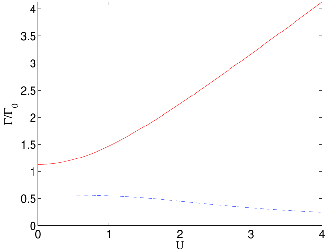
Figure 1: (Color online) The total transition rate $\Gamma(U)$ for a constant cross section [Eq. (31)] (continuous line) and for a Gaussian cross section with $a=1$ [Eq. (34)] (broken line).

For the case of a constant scattering cross section,

$$\sigma(K)=\sigma=\mbox{const},$$ (30)

the total transition rate is found to be

$$\Gamma(U)=\Gamma_{0}\left\{\left[1+2U^{2}\right]\frac{{\mathrm{erf}}(U)}{2U}+\frac{1}{\sqrt{\pi}}e^{-U^{2}}\right\},$$ (31)

where the quantity

$$\Gamma_{0}=n_{\mathrm{gas}}v_{\mathrm{mp}}4\pi\sigma$$ (32)

represents the total scattering rate corresponding to an incoming flux of particles with the most probable velocity $v_{\mathrm{mp}}$. For a Gaussian scattering cross section of the form

$$\sigma(K)=\sigma\,e^{-aK^{2}/4}$$ (33)

one has instead

$$\Gamma(U)=\frac{\Gamma_{0}}{aU}\left\{{\mathrm{erf}}(U)-\frac{\mathrm{erf}(U/\sqrt{a+1})}{\sqrt{a+1}}e^{-\frac{a}{a+1}U^{2}}\right\}.$$ (34)

The form of these functions is illustrated in Fig. 1. One observes that for large $U$ the function $\Gamma(U)$ increases linearly with $U$ in the case of a constant cross section, while it decreases as $U^{-1}$ in the case of a Gaussian cross section. We note also that in terms of the scaled momentum variables the canonical mean value $\langle{\mathbf{P}}^{2}/2M\rangle_{\mathrm{eq}}={3}/2\beta$ of the kinetic energy of the test particle reached at thermal equilibrium corresponds to $\langle{\mathbf{U}}^{2}\rangle_{\mathrm{eq}}=3m/2M$.

IV Numerical algorithms and simulation results

IV.1 Dissipative effects

We first study relaxation to thermal equilibrium by considering the dynamics of an ensemble of momentum eigenstates of a test particle in a Maxwell-Boltzmann gas. Hence, using the scaled momentum variables introduced in Sec. II we investigate initial states of the form

$$|\psi(0)\rangle=|{\mathbf{U}}(0)\rangle.$$ (35)

The application of the quantum jump unravelling described in Sec. III then leads to a classical stochastic process ${\mathbf{U}}(t)$ for the test particle momentum. This process is a pure jump process the realizations of which are obtained through the algorithm described below. Note that this algorithm corresponds to the standard algorithm that is used for the stochastic simulation of classical Markovian master equations Gillespie (1992). In order to study relaxation to a Gaussian thermal state we will consider the behavior in time of first and second moments of the momentum distribution, as well as of various cumulants of the distribution.

IV.1.1 Simulation method

The state ${\mathbf{U}}(0)$ at the initial time $t=0$ is to be drawn from a given distribution for the initial data. Suppose a jump occurred at some time $t_{0}$ leading to the state ${\mathbf{U}}(t_{0})\equiv{\mathbf{U}}$. The next jump will then take place at time $t_{0}+\tau$, where $\tau$ is a stochastic time step which is given by

$$\tau=-\frac{1}{\Gamma(U)}\ln\eta.$$ (36)

$\eta$ is a random number which is uniformly distributed over the interval $(0,1)$, and $\Gamma(U)$ represents the total transition rate. Since the process is a pure jump process, ${\mathbf{U}}$ stays constant between $t_{0}$ and $t_{0}+\tau$.

At time $t_{0}+\tau$ one carries out a jump by replacing

$${\mathbf{U}}\longrightarrow{\mathbf{U}}+\frac{m_{*}}{M}{\mathbf{K}}.$$ (37)

The momentum transfer ${\mathbf{K}}$ is determined as follows. First, one draws random numbers $(K,\xi)$ that follow the joint probability density $R(K,\xi)$ which is normalized as

$$\int_{0}^{\infty}dK\int_{-1}^{+1}d\xi\,R(K,\xi)=1.$$ (38)

$K$ is the size of the momentum transfer and $\xi$ the cosine of the angle between ${\mathbf{K}}$ and ${\mathbf{U}}$. In the Monte Carlo simulations shown below we have used the rejection method to determine $(K,\xi)$. Second, one draws a uniformly distributed random unit vector ${\mathbf{e}}$. Then, the momentum transfer is given by the formula

$${\mathbf{K}}={\mathbf{K}}_{\parallel}+{\mathbf{K}}_{\perp}=K\xi\frac{\mathbf{U}}{U}+K\sqrt{1-\xi^{2}}\frac{{\mathbf{U}}\times{\mathbf{e}}}{|{\mathbf{U}}\times{\mathbf{e}}|}.$$ (39)

${\mathbf{K}}_{\parallel}$ is the component of ${\mathbf{K}}$ which is parallel to the particle momentum ${\mathbf{U}}$, and ${\mathbf{K}}_{\perp}$ its component perpendicular to it. Repeating these steps until the desired final time $t_{f}$ is reached one obtains a realization of the process ${\mathbf{U}}(t)$ over the whole time interval $[0,t_{f}]$.

IV.1.2 Constant scattering cross section

We first address momentum and energy relaxation for the case of a constant scattering cross section $\sigma$. The corresponding total transition rate $\Gamma(U)$ is given by Eq. (31), while the joint probability of $(K,\xi)$ takes the form

$$R(K,\xi)=\frac{\Gamma_{0}}{2\sqrt{\pi}\Gamma(U)}K\exp\left[-\left(\frac{K}{2}+U\xi\right)^{2}\right].$$ (40)

This probability density is illustrated in Fig. 2. For small $U$ the density $R(K,\xi)$ is nearly uniform in $\xi$, corresponding to an isotropic distribution, while it has a pronounced maximum at $\xi=-1$ if $U$ is not small. In the latter case there is thus a strong tendency that the momentum transfer ${\mathbf{K}}$ is opposite to the direction of the particle momentum ${\mathbf{U}}$.

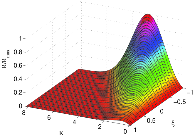
Figure 2: (Color online) The probability density $R(K,\xi)$ given by Eq. (40) for $U=1$.

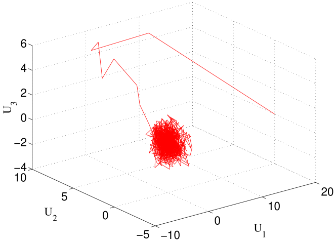
Figure 3: (Color online) A single realization of the process ${\mathbf{U}}(t)$ for $m/M=1$.

Figure 3 shows a single realization of the process ${\mathbf{U}}(t)$ as a 3D plot. One observes that already a few momentum kicks drive the test particle into the vicinity of the equilibrium value. Statistical estimates for the quantities $\langle{\mathbf{U}}(t)\rangle^{2}$ and $\langle{\mathbf{U}}(t)^{2}\rangle$ for various values of $m/M$ are shown in Figs. 4, 5 and 6. In these simulations we have taken a sharp initial state proportional to $(1,0,0)$. We see a nice relaxation to the respective equilibrium values $\langle{\mathbf{U}}\rangle^{2}_{\mathrm{eq}}=0$ and $\langle{\mathbf{U}}^{2}\rangle_{\mathrm{eq}}=3m/2M$ for all parameter combinations used.

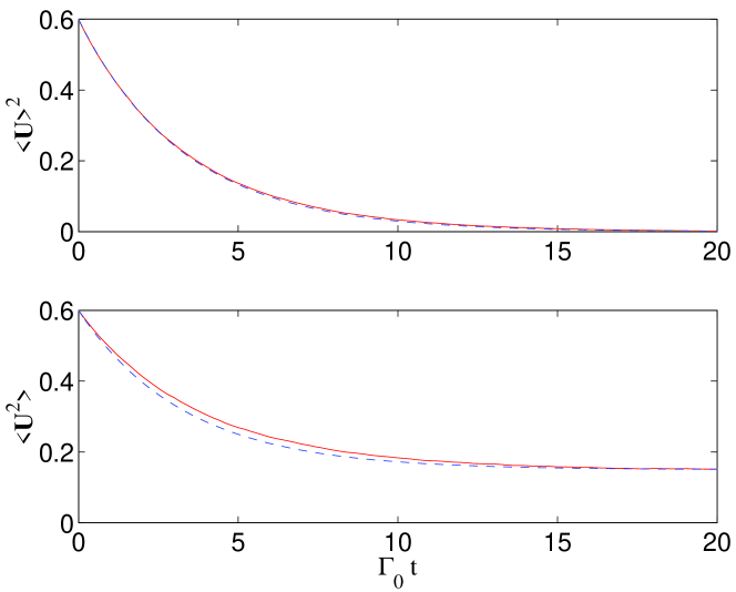
Figure 4: (Color online) Averages over $10^{4}$ realizations for a constant cross section and $m/M=0.1$. The broken lines represent the approximate relaxation dynamics according to Eqs. (41) and (42), respectively.

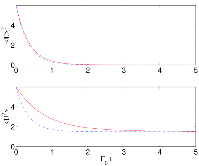
Figure 5: (Color online) The same as Fig. 4 for $m/M=1$.

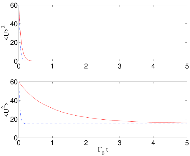
Figure 6: (Color online) The same as Fig. 4 for $m/M=10$.

A simple approximation of the relaxation dynamics can be obtained in the limiting case $m/M\ll 1$. According to Ref. Vacchini and Hornberger (to appear) one then finds

$$\langle{\mathbf{U}}(t)\rangle^{2}\approx\langle{\mathbf{U}}(0)\rangle^{2}e^{-\gamma_{R}t}$$ (41)

and

$$\langle{\mathbf{U}}^{2}(t)\rangle\approx\left[\langle{\mathbf{U}}^{2}(0)\rangle-\langle{\mathbf{U}}^{2}\rangle_{\mathrm{eq}}\right]e^{-\gamma_{R}t}+\langle{\mathbf{U}}^{2}\rangle_{\mathrm{eq}},$$ (42)

where the relaxation rate is given by

$$\gamma_{R}=\frac{16}{3\sqrt{\pi}}\frac{m}{M}\Gamma_{0}.$$ (43)

We see from the figures that the dynamics of the mean squared momentum $\langle{\mathbf{U}}^{2}(t)\rangle$ strongly deviates from these approximations if $m/M$ is not small, while the behavior of the squared mean momentum $\langle{\mathbf{U}}(t)\rangle^{2}$ is still well approximated by Eq.(43). A further characteristic feature is that for $m/M\gg 1$ the squared mean momentum $\langle{\mathbf{U}}(t)\rangle^{2}$ decays much faster than the mean squared momentum $\langle{\mathbf{U}}^{2}(t)\rangle$. This means that the relaxation of the momentum and of the kinetic energy of the particle are characterized by different decay times, by contrast to typical master equations for quantum Brownian motion.

IV.1.3 Gaussian scattering cross section

For a Gaussian scattering cross section of the form $\sigma(K)=\sigma\exp[-aK^{2}/4]$ the total transition rate was given in Eq. (34). The corresponding joint probability density becomes

$$R(K,\xi)=\frac{\Gamma_{0}}{2\sqrt{\pi}\Gamma(U)}K\exp\left[-\left(\frac{K}{2}+U\xi\right)^{2}-\frac{a}{4}K^{2}\right].$$ (44)

The qualitative features of this density are the same as for the case of a constant cross section. Simulation results for $m/M=1$ and $a=1$ are shown in Fig. 7. As expected we see the relaxation to the equilibrium values predicted by the stationary solution. In the case $m/M\ll 1$ the approximations given by Eqs. (41) and (42) are again valid, where the relaxation rate now takes the form

$$\gamma_{R}=\frac{16}{3\sqrt{\pi}}\frac{m}{M}\frac{1}{(1+a)^{2}}\Gamma_{0}.$$ (45)

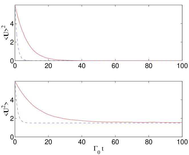
Figure 7: (Color online) Averages over $10^{4}$ realizations for a Gaussian cross section with $m/M=1$ and $a=1$. The broken lines represent the approximate relaxation dynamics with the rate given by Eq. (45).

IV.1.4 Cumulants of higher order

The stochastic process ${\mathbf{U}}(t)$ describing the particle momentum is nonlinear in the sense that large non-Gaussian fluctuations are dynamically generated. Starting from a Gaussian initial state we end up for long times with a Gaussian final (equilibrium) state. However, for intermediate times one observes strong deviations from Gaussian statistics.

To investigate these deviations one has to consider higher moments of the components $U_{i}(t)$, $i=1,2,3$, of the test particle momentum. To this aim we have determined the time-dependence of the cumulants of second, third and fourth order (summed over the components of the momentum),

$$\kappa_{2} = \sum_{i}\left\langle(U_{i}-\langle U_{i}\rangle)^{2}\right\rangle,$$ (46)

$$\kappa_{3} = \sum_{i}\left\langle(U_{i}-\langle U_{i}\rangle)^{3}\right\rangle,$$ (47)

$$\kappa_{4} = \sum_{i}\left[\left\langle(U_{i}-\langle U_{i}\rangle)^{4}\right\rangle-3\left\langle(U_{i}-\langle U_{i}\rangle)^{2}\right\rangle^{2}\right].$$ (48)

For a Gaussian distribution all cumulants of order larger than two vanish identically. Simulation results are shown in Fig. 8. We indeed see the emergence of large non-Gaussian fluctuations for which the cumulants $\kappa_{3}$ and $\kappa_{4}$ are of the same order of magnitude as the variance $\kappa_{2}$.

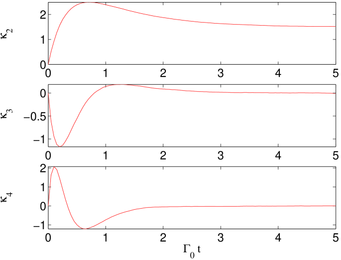
Figure 8: (Color online) Cumulants of second, third and fourth order obtained from averages over $10^{5}$ realizations for a constant cross section and $m/M=1$.

IV.2 Decoherence effects

As mentioned in Sec. II diagonal matrix elements in the momentum representation of the quantum linear Boltzmann equation coincide with the classical expression. Typical quantum features are therefore linked to the off-diagonal matrix elements and their behavior in time. The suppression of these matrix elements corresponds to a transition from the quantum to the classical regime. It is therefore of interest to consider the evolution in time of a superposition state. As argued in Sec. III superpositions of momentum eigenstates are preserved in the course of the time evolution. This implies that an initial state of the form

$$|\psi(0)\rangle=\sum_{i=1}^{N}\alpha_{i}(0)|\mathbf{U}_{i}(0)\rangle,$$ (49)

where the amplitudes satisfy the normalization condition $\sum_{i=1}^{N}|\alpha_{i}(0)|^{2}=1$, can be expressed at time $t$ as

$$|\psi(t)\rangle=\sum_{i=1}^{N}\alpha_{i}(t)|\mathbf{U}_{i}(t)\rangle.$$ (50)

The stochastic state vector is therefore uniquely fixed by $N$ momenta $\{\mathbf{U}_{i}(t)\}_{i=1\ldots N}$ and $N$ complex amplitudes $\{\alpha_{i}(t)\}_{i=1\ldots N}$ obeying the normalization condition $\sum_{i=1}^{N}|\alpha_{i}(t)|^{2}=1$ for any $t$.

IV.2.1 Simulation method

Suppose that at time $t_{0}$ a jump into the state

$$|\psi(t_{0})\rangle=\sum_{i=1}^{N}\alpha_{i}(t_{0})|\mathbf{U}_{i}(t_{0})\rangle$$ (51)

occurred. The deterministic time evolution before the next jump generated by the effective Hamiltonian (11) is described by

$$|\psi(t_{0}+\tau)\rangle=\sum_{i=1}^{N}\alpha_{i}(t_{0}+\tau)|\mathbf{U}_{i}(t_{0})\rangle.$$ (52)

Hence, the momenta ${\mathbf{U}}_{i}$ stay constant while the dynamics of the amplitudes is given by

$$\alpha_{i}(t_{0}+\tau)=\frac{e^{-iE(U_{i}(t_{0}))\tau/\hbar}e^{-\Gamma(U_{i}(t_{0}))\tau/2}}{\sqrt{\sum_{j}|\alpha_{j}(t_{0})|^{2}e^{-\Gamma(U_{j}(t_{0}))\tau}}}\alpha_{i}(t_{0}),$$ (53)

where $E(U)=P^{2}/2M=Mv_{\mathrm{mp}}^{2}U^{2}/2$. The waiting time distribution $F(\tau)$ for the next jump is now represented by a sum of exponential functions,

$$F(\tau)=1-\sum_{i=1}^{N}|\alpha_{i}(t_{0})|^{2}e^{-\Gamma(U_{i}(t_{0}))\tau}.$$ (54)

The jump at time $t=t_{0}+\tau$ is described by the replacements

$${\mathbf{U}}_{i}(t_{0}) \longrightarrow {\mathbf{U}}_{i}(t_{0})+\frac{m_{*}}{M}{\mathbf{K}},$$ (55)

$$\alpha_{i}(t_{0}+\tau) \longrightarrow f_{i}\alpha_{i}(t_{0}+\tau),$$ (56)

where the factors $f_{i}$ are given by

$$f_{i}=\frac{e^{-\frac{1}{2}\left(K/2+{\mathbf{K}}\cdot{\mathbf{U}_{i}(t_{0})}/K\right)^{2}}}{\sqrt{\sum_{j}|\alpha_{j}(t_{0}+\tau)|^{2}e^{-\left(K/2+{\mathbf{K}}\cdot{\mathbf{U}_{j}(t_{0})}/K\right)^{2}}}}.$$ (57)

The momentum transfer ${\mathbf{K}}$ in these formulas is to be drawn from the corresponding probability density $R({\mathbf{K}})$. To determine ${\mathbf{K}}$ one proceeds as follows. First, one draws an index $i\in\{1,2,\ldots,N\}$ with probability

$$p_{i}=\frac{|\alpha_{i}(t_{0})|^{2}e^{-\Gamma(U_{i}(t_{0}))\tau}\Gamma(U_{i}(t_{0}))}{\sum_{j}|\alpha_{j}(t_{0})|^{2}e^{-\Gamma(U_{j}(t_{0}))\tau}\Gamma(U_{j}(t_{0}))}.$$ (58)

Given $i$ one then draws a momentum transfer ${\mathbf{K}}$ that follows the probability density $R(K,\xi_{i})$ [see Eq. (40)], where now $\xi_{i}$ represents the cosine of the angle between ${\mathbf{K}}$ and ${\mathbf{U}}_{i}(t_{0})$.

IV.2.2 Decay of coherences

We have used the simulation algorithm described above to study the loss of coherence of an initial state of the form

$$|\psi(0)\rangle=\alpha_{1}(0)|{\mathbf{U}}_{1}(0)\rangle+\alpha_{2}(0)|{\mathbf{U}}_{2}(0)\rangle,$$ (59)

given by a superposition of two momentum eigenvectors. The initial state is to be drawn from a given initial distribution for the momenta ${\mathbf{U}}_{1,2}(0)$ and amplitudes $\alpha_{1,2}(0)$. In the simulations shown below we have taken sharp opposite initial momenta,

$${\mathbf{U}}_{1}(0)=-{\mathbf{U}}_{2}(0)\equiv{\mathbf{U}}_{0},$$ (60)

and equal amplitudes,

$$\alpha_{1}(0)=\alpha_{2}(0)=\frac{1}{\sqrt{2}}.$$ (61)

Such an initial state is a balanced coherent superposition of two momentum eigenvectors separated by twice $U_{0}\equiv\Delta P/p_{\mathrm{mp}}$, where $p_{\mathrm{mp}}=mv_{\mathrm{mp}}$ is the most probable momentum of the gas particle at temperature $T=1/k_{\text{B}}\beta$. In order to study quantitatively the loss of coherence we have used the simulation algorithm to estimate the expectation value

$$C(t)={\mathbb{E}}\left[\frac{|\alpha_{1}(t)\alpha_{2}^{*}(t)|}{|\alpha_{1}(0)\alpha_{2}^{*}(0)|}\right]=2{\mathbb{E}}\left[|\alpha_{1}(t)\alpha_{2}^{*}(t)|\right].$$ (62)

This quantity represents the average of the absolute values of the coefficients in front of the off-diagonal matrix elements of the test particle’s statistical operator in the momentum representation, divided by its initial value. Hence, $C(t)$ provides a measure for the degree of the coherence of the state of the test particle. An example for the dynamical behavior of $C(t)$ is shown in Fig. 9. In this figure we have used a sharp initial state given by ${\mathbf{U}}_{0}=(0,0,4)$. We clearly see an exponential decay of the coherence $C(t)$ over several orders of magnitude.

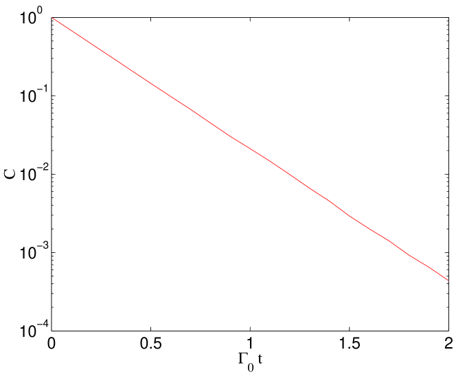
Figure 9: (Color online) Semilogarithmic plot of the coherence $C(t)$ obtained from an average over $10^{5}$ realizations for $m/M=1$ (constant cross section).

Assuming that an exponential decay of the coherence holds true, we define the decoherence rate $\gamma_{D}$ by means of

$$C(t)=e^{-\gamma_{D}t}.$$ (63)

An analytical approximation for $\gamma_{D}$ can be found with the help of the following argument. We take a sufficiently small time $t$ such that we can approximate

$$C(t)\approx 1-\gamma_{D}t\approx 1-\Gamma(U_{0})t+\Gamma(U_{0})t\langle f_{1}f_{2}\rangle.$$ (64)

Here, $\Gamma(U_{1}(0))=\Gamma(U_{2}(0))=\Gamma(U_{0})$ represents the total rate for a transition out of the given initial state (59). Hence, $\Gamma(U_{0})t$ represents the probability for a jump within time $t$, while $1-\Gamma(U_{0})t$ is the probability that no jump occurs. Using Eqs. (60) and (61) we see from Eq. (53) that $C$ does not change during the deterministic drift. On the other hand, if a jump does occur then $C$ changes from its initial value $C=1$ to $C=f_{1}f_{2}$ as may be seen from Eq. (56). According to Eq. (57) we have

$$f_{1}f_{2}=\frac{2}{e^{{\mathbf{K}}\cdot{\mathbf{U}}_{0}}+e^{-{\mathbf{K}}\cdot{\mathbf{U}}_{0}}}.$$ (65)

Thus, Eq. (64) represents the change of $C$ as a result of two alternatives, namely that a jump does occur or that it does not (for small enough $t$ we can have at most one jump). Finally, $\langle f_{1}f_{2}\rangle$ denotes the average of $f_{1}f_{2}$ taken over the possible momentum transfers during the first jump. We therefore get

$$\gamma_{D} \approx \Gamma(U_{0})(1-\langle f_{1}f_{2}\rangle)$$ (66)

$$= \Gamma(U_{0})\left\langle 1-\mathrm{Sech}({{\mathbf{K}}\cdot{\mathbf{U}}_{0}})\right\rangle.$$

This formula can be analytically evaluated in several cases. For a constant scattering cross section one finds exploiting Eq. (40),

$$\gamma_{D}=\Gamma(U_{0})-\Gamma_{0}\frac{\mathrm{erf}(U_{0})}{U_{0}}.$$ (67)

Fig. 10 demonstrates the extremely good agreement between the stochastic simulation results and this analytical approximation. The Monte Carlo estimates for the decoherence rate have been obtained by least squares fits to the simulation data within the time interval in which the coherence decays to $1\%$ of its initial value. For all cases shown we find a nearly perfect exponential decay. Our argument shows that it is just the real scattering events that mainly cause the decoherence during the early phase of the dynamics, by contrast to the virtual transitions described by the non-Hermitian drift Hamiltonian.

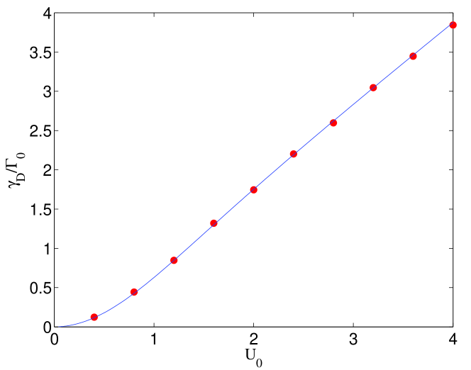
Figure 10: (Color online) The decoherence rate $\gamma_{D}$ in units of $\Gamma_{0}$ as a function of the initial momentum $U_{0}$. Points: Least squares fits of the simulation data for $m/M=1$. Continuous line: Analytical estimate given by Eq. (67).

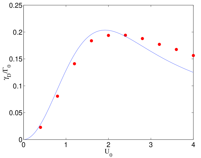
Figure 11: (Color online) The same as Fig. 10 for a Gaussian cross section with $a=1$. The continuous line represents the analytical estimate given by Eq. (68).

For a Gaussian cross section Eq. (66) leads to

$$\gamma_{D}=\Gamma(U_{0})-\Gamma_{0}\frac{\mathrm{erf}(U_{0})}{U_{0}}\frac{1}{1+a}.$$ (68)

In Fig. 11 we compare this expression with the simulation results. Although the quantitative agreement is obviously not as good as in the case of a constant cross section, the analytical formula (68) still yields a reasonable estimate for the order of magnitude of the decoherence rate.

The above results enable us to study the relationship between the time scales characterizing the different physical phenomena. For the case of $m/M\ll 1$ the time scale for relaxation is given by Eq. (43). Considering a wide separation in momentum of the initial superposition on the scale set by the momentum of the gas particles, so that $U_{0}=\Delta P/p_{\mathrm{mp}}\gg 1$, one can consider the corresponding limiting value $\Gamma_{0}U_{0}$ of Eq. (67), and the ratio of the decoherence rate to the relaxation rate is given by

$$\frac{\gamma_{D}}{\gamma_{R}}\approx\frac{3\sqrt{\pi}}{16}\frac{M}{m}U_{0}\gg 1.$$ (69)

This shows that the decoherence time $\gamma_{D}^{-1}$ for the loss of coherence in momentum space can be much smaller than the relaxation time $\gamma_{R}^{-1}$, i. e. than the time it takes for the relaxation of the energy of the test particle.

It is also of interest to compare the relaxation timescale with the decoherence rate $\eta_{D}$ of a superposition of position eigenstates, widely separated on the scale set by the thermal wavelength of the gas particles, which corresponds to $\hbar$ divided by the typical momentum transfer, so that $\Delta X/\lambda_{\mathrm{th}}\gg 1$. In such a case for $m/M\ll 1$ the decoherence rate is set by the total transition rate Joos and Zeh (1985); Gallis and Fleming (1990); Hornberger et al. (2003); Hornberger and Sipe (2003); Vacchini (2004, 2005), so that for a test particle much slower than the gas particles one has $\eta_{D}\approx 2\Gamma_{0}/\sqrt{\pi}$. Thus, the ratio

$$\frac{\eta_{D}}{\gamma_{R}}\approx\frac{3}{8}\frac{M}{m}\gg 1$$ (70)

shows again that the decoherence time $\eta_{D}^{-1}$ for the loss of coherence in position space can be much smaller than the relaxation time $\gamma_{R}^{-1}$, but still longer than the decoherence time in momentum space $\gamma_{D}^{-1}$.

V Conclusions

We have developed a stochastic unravelling of the quantum linear Boltzmann equation which leads to an efficient Monte Carlo simulation technique, despite the appearance in the equation itself of quite complicated operator-valued expressions. The latter are responsible for deviations from Gaussian statistics, at variance with typical master equations used for the description of quantum Brownian motion. A crucial feature of the method is that the developed algorithms fully exploit the translation covariance and thus allow full three-dimensional stochastic simulations of the quantum Boltzmann equation. In particular, the method does not require the introduction of a discretization in momentum space, so that the continuous sum over the Lindblad operators in Eq. (9) can be exactly accounted for.

The method proposed here suggests many further physically relevant applications. For example, one can extend the algorithm to the regime where effects from the Bose or Fermi statistics of the quantum gas come into play. In fact, starting from Eqs. (4) and (5) one can analytically work out the corresponding expressions of the dynamic structure factor for a free gas of particles obeying Bose or Fermi statistics, coming to Vacchini (2001a)

$$S_{\rm\scriptscriptstyle B/F}(Q,E) = \frac{1}{(2\pi\hbar)^{3}}\frac{2\pi m^{2}}{n_{\mathrm{gas}}\beta Q}\frac{\mp 1}{1-e^{\beta E}}$$

$$\times\ln\left[\frac{1\mp z\exp\left[-\frac{\beta}{8m}\frac{(2mE+Q^{2})^{2}}{Q^{2}}\right]}{1\mp z\exp\left[-\frac{\beta}{8m}\frac{(2mE-Q^{2})^{2}}{Q^{2}}\right]}\right],$$

where the upper signs refer to the Bose case and the lower signs to the Fermi case, and $z$ denotes the fugacity of the gas. By use of this expression the algorithm thus enables Monte Carlo simulations of the behavior of test particles in a Bose or Fermi gas to identify genuine effects of the quantum statistics. More generally, the method may also be applied to an interacting quantum gas provided an (at least approximate) expression for the dynamic structure factor $S({\mathbf{Q}},{\mathbf{P}})$ is known.

A further example is the investigation of the important problem of decoherence in position space. This can be done by use of initial states representing superpositions of localized wave packets, with the aim of determining the corresponding position space decoherence time scales. Localized wave packets may of course be represented by introducing a discretization of position space. However, it seems that it is much more efficient to invoke the translation covariance and to describe spatially localized states by appropriate superpositions of momentum eigenstates as discussed in Sec. IV.2, or, more generally, by superpositions of wave packets localized in momentum space. Further examples of application include the extension of the method to the determination of multitime correlation functions, to the treatment of particles with internal degrees of freedom, and to the case of an operator-valued scattering amplitude, i. e. to the case that the scattering cross section depends on the momentum of the incoming test particle.