On the Polyphase Decomposition for Design of Generalized Comb Decimation Filters

Abstract

Generalized comb filters (GCFs) are efficient anti-aliasing decimation filters with improved selectivity and quantization noise (QN) rejection performance around the so called folding bands with respect to classical comb filters.

In this paper, we address the design of GCF filters by proposing an efficient partial polyphase architecture with the aim to reduce the data rate as much as possible after the $\Sigma\Delta$ A/D conversion. We propose a mathematical framework in order to completely characterize the dependence of the frequency response of GCFs on the quantization of the multipliers embedded in the proposed filter architecture. This analysis paves the way to the design of multiplier-less decimation architectures.

We also derive the impulse response of a sample $3$rd order GCF filter used as a reference scheme throughout the paper.

I Introduction and problem formulation

The design of computationally efficient decimation filters for $\Sigma\Delta$ A/D converters is a well-known research topic [1, 2, 3]. Given a base-band analog input signal $x(t)$ with bandwidth $\left[-f_{x},+f_{x}\right]$, a $\Sigma\Delta$ A/D converter of order $B$ produces a digital signal $x(nT_{s})$ by sampling $x(t)$ at rate $f_{s}=2\rho f_{x}\gg 2f_{x}$, whereby $\rho$ is the so called oversampling ratio. The normalized maximum frequency contained in the input signal is defined as $f_{c}=\frac{f_{x}}{f_{s}}=\frac{1}{2\rho}$, and the digital signal $x(nT_{s})$ at the input of the first decimation filter has frequency components belonging to the range $f_{d}\in[-f_{c},f_{c}]$ (where $f_{d}$ denotes the digital frequency). This setup is pictorially depicted in the reference architecture shown in Fig. 1.

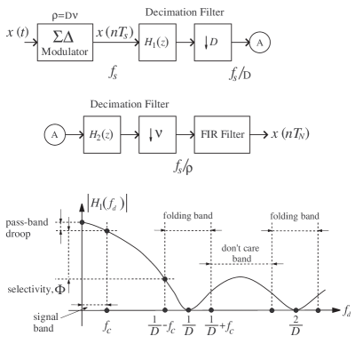
Figure 1: General architecture of a two-stage decimation chain for $\Sigma\Delta$ A/D converters, along with a pictorial representation of the key frequency intervals to be carefully considered for the design of the first decimation stage.

Owing to the condition $\rho\gg 1$, the decimation of an oversampled signal $x(nT_{s})$ is efficiently [4] accomplished by cascading two (or more) decimation stages, as highlighted in Fig. 1, followed by a FIR filter which provides the required selectivity on the sampled signal $x(nT_{N})$ at baseband. The first decimation filter is usually an $N$-th order comb filter decimating by $D$ [2, 3, 5], whereby the order $N$ has to be greater or equal to $B+1$ [1, 3].

The design of a multistage decimation filter for $\Sigma\Delta$ converters poses stringent constraints on the shape of the frequency response of the first decimation stage. Considering the scheme in Fig. 1, the frequency response $H_{1}(e^{j\omega})$ of the first decimation filter must attenuate the QN falling inside the so called folding bands, i.e. the frequency ranges defined as $\left[\frac{k}{D}-f_{c};\frac{k}{D}+f_{c}\right]$ with $k=1,...,\lfloor\frac{D}{2}\rfloor$ if $D$ is even, and $k=1,...,\lfloor\frac{D-1}{2}\rfloor$ for $D$ odd (for conciseness, the set of values assumed by $k$ will be denoted as $K_{k}$ throughout the paper). The reason is that the $\Sigma\Delta$ QN falling inside these frequency bands, will fold down to baseband because of the sampling rate reduction by $D$ in the first decimation stage, irremediably affecting the signal resolution after the multistage decimation chain. This issue is especially important for the first decimation stage, since the QN folding down to baseband has not been previously attenuated. Fig. 1 also shows the frequency range $\left[0,f_{c}\right]$ where the useful signal bandwidth falls, along with the so called don’t care bands, i.e. the frequency ranges whose QN will be rejected by the filters placed beyond the first decimation stage.

In connection with the first decimation stage in the multistage architecture shown in Fig. 1, the required aliasing protection around the folding bands is usually guaranteed by a comb filter, which provides an inherent antialising function by placing its zeros in the middle of each folding band. We recall that the transfer function of a $N$-th-order comb filter is defined as [2]:

$$\small H_{C_{N}}(z)=\left(\frac{1}{D}\frac{1-z^{-D}}{1-z^{-1}}\right)^{N}=\frac{1}{D^{N}}\prod_{i=1}^{D-1}\left(1-z^{-1}e^{j\frac{2\pi}{D}i}\right)^{N}$$ (1)

where $D$ is the desired decimation factor.

With this background, let us provide a quick survey of the recent literature related to the problem addressed here. This survey is by no means exhaustive and is meant to simply provide a sampling of the literature in this fertile area.

A $3$rd order modified decimation sinc filter was proposed in [6], and still further analyzed in [7, 8]. The class of comb filters was then generalized in [9], whereby the authors proposed an optimization framework for deriving the optimal zero rotations of GCFs for any filter order and decimation factor $D$.

Other works somewhat related to the topic addressed in this paper are [10]-[15]. In [10] and [11] authors proposed computational efficient decimation filter architectures for implementing classical comb filters. In [12] authors proposed the use of decimation sharpened filters embedding comb filters, whereas in [13] authors addressed the design of a novel two-stage sharpened comb decimator. In [14], authors proposed novel decimation schemes for $\Sigma\Delta$ A/D converters based on Kaiser and Hamming sharpened filters, then generalized in [15] for higher order decimation filters.

The main aim of this paper is to propose a flexible, yet effective, partial polyphase architecture for implementing the GCF filters proposed in the companion paper [9]. To this end, we first recall the $z$-transfer function of GCF filters for completeness, and, then, provide a mathematical formulation for deriving the impulse response of this class of decimation filters. The latter is needed for deriving the polyphase components of the proposed filters. In the second part of the paper, the focus is on the sensitivity of the frequency response of GCF filters due to the quantization of the multipliers embedded in the proposed architecture. We also analyze zero displacements in the $z$-transfer function of GCF filters for deducing useful hints at the basis of any practical implementation of such filters.

The rest of the paper is organized as follows. In Section II, we briefly recall the transfer functions of GCF filters and highlight their main peculiarities with respect to classical comb filters. Section III presents an effective architecture, namely a partial polyphase decomposition, for implementing GCF decimation filters; the impulse response of a sample $3$rd order GCF filter is also presented, and mathematically derived in the Appendix. In Section IV, we present a mathematical framework for evaluating the sensitivity of the frequency response of GCF filters to the approximations of the embedded multipliers. Zero displacements due to multiplier approximation is discussed in Section V, where we also draw general guidelines for the design of such filters. Finally, Section VI draws the conclusions.

II The $z$-Transfer function of GCF filters

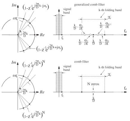
Figure 2: Zero locations of the considered decimation filters within the $k$-th folding band. Zeros are displayed in the $z$-plane and in the frequency axis in order to highlight their effect in both domains.

In this section, we briefly recall the $z$-transfer function of GCF filters proposed in [9]. The $z$-transfer function $H_{GCF_{N}}(z)$ of a $N$-th order GCF filter decimating by $D$ is defined as:

$$\small\frac{1}{H_{o,ev,1}}H_{1}(z) \cdot\prod_{n=1}^{\left\lfloor\frac{N}{2}\right\rfloor}H_{2}(z,\alpha_{n+N}), D~{}even,~{}N~{}even$$

$$\frac{\left(1+z^{-1}\right)}{H_{o,ev,2}}H_{1}(z) \cdot\prod_{n=1}^{\left\lfloor\frac{N}{2}\right\rfloor}H_{2}(z,\alpha_{n+N}), D~{}even,~{}N~{}odd$$

$$\frac{1}{H_{o,od}}H_{1}(z), D~{}odd$$ (2)

whereby the involved basic functions are defined as follows:

$$\small\begin{array}[]{ll}H_{1}(z)=\prod_{i=1}^{D_{M}}\prod_{n=1}^{N}\left(1-2\cos\left(\frac{2\pi}{D}i-\alpha_{n}\right)z^{-1}+z^{-2}\right),&\\ =\prod_{i=1}^{D_{M}}\prod_{n=1}^{N}\left(1-z^{-1}e^{+j\frac{2\pi}{D}i-j\alpha_{n}}\right)\left(1-z^{-1}e^{-j\frac{2\pi}{D}i+j\alpha_{n}}\right)&\end{array}$$ (3)

with $D_{M}=\frac{D}{2}-1$, for $D$ even, and $D_{M}=\frac{D-1}{2}$, for $D$ odd, and

$$H_{2}(z,\alpha_{n+N})=1-2\cos\left(\pi-\alpha_{n+N}\right)z^{-1}+z^{-2}$$ (4)

Terms $H_{o,ev,1}$, $H_{o,ev,2}$, and $H_{o,od}$ are appropriate normalization constants chosen in such a way as to have $\left.H_{GCF_{N}}(z)\right|_{z=1}=1$, and $\left\lfloor\cdot\right\rfloor$ is the floor of the underlined number.

Let us summarize the main peculiarities of GCF filters by comparing them to classical comb filters. GCFs are, as comb filters, linear-phase filters since they are constituted by two linear-phase basic filters, namely $H_{1}(z)$ and $H_{2}(z)$.

An $N$-th order comb filter (1) decimating by $D$, places $N$-th order zeros in the complex locations $z_{i}=e^{j\frac{2\pi}{D}i},~{}\forall i=1,\ldots,D-1$, or, equivalently, in the digital frequencies $f_{z_{k}}=\frac{k}{D},~{}k\in K_{k}$. On the other hand, an $N$-th order GCF filter decimating by $D$ places $N$ pairs of conjugate complex zeros in the $i$-th folding band, with $i=1,\ldots,D_{M}$, as exemplified by the function $H_{1}(z)$ in (II). A pictorial representation of the zero locations of a GCF filter is given in Fig. 2. The behaviour of the function $H_{2}(z)$ is analogous to that of $H_{1}(z)$ with the exception that its zeros are placed around the location $z=-1$ in the $z$-complex plane, and, it holds only for $D$ even. A convenient choice for $\alpha_{p}$ is $\alpha_{p}=q_{p}2\pi f_{c},$ with $q_{p}\in\left[-1,+1\right]$: this solution is such that each pair of conjugate complex zeros falls inside the relative folding band guaranteeing the required selectivity in these frequency bands. By virtue of the zero distribution within the folding bands, GCF filters provide improved $\Sigma\Delta$ QN rejection capabilities with respect to classical comb filters of the same order. For completeness, Table I shows the optimal zero rotations $q_{p}$s found in [9] by minimizing the $\Sigma\Delta$ QN around the folding bands. As an example, a $3$rd order GCF filter provides a $\Sigma\Delta$ QN rejection $8$dB higher than that guaranteed by a classical $3$rd order comb filter. Throughout the paper we will use this optimal choice of the zero rotations where no otherwise specified. We invite the interested readers to refer to [9] for further details about the characteristics along with the performance of GCF filters.

TABLE I: Optimal parameters of GCF decimation filters.

$N$	$3$	$4$	$5$	$6$
$q_{1}$	-0.79	-0.35	+0.55	+0.95
$q_{2}$	0.0	+0.35	+0.93	+0.675
$q_{3}$	+0.79	-0.88	-0.55	+0.25
$q_{4}$	+0.79	+0.88	-0.93	-0.25
$q_{5}$	-	+0.88	0.0	-0.675
$q_{6}$	-	+0.35	+0.55	-0.95
$q_{7}$	-	-	+0.93	+0.95
$q_{8}$	-	-	-	+0.675
$q_{9}$	-	-	-	+0.25
$G-[dB]$	$\sim$8	$\sim$13	$\sim$18	$\sim$ 23

III Partial Polyphase Decomposition of GCF Filters

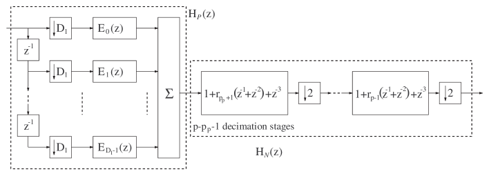
Figure 3: Architecture of the partial polyphase implementation of the decimation filter $H_{GCF_{3}}(z)$. The overall decimation factor $D=D_{1}\cdot D_{2}$ is split between the polyphase section decimating by $D_{1}=2^{p_{p}+1}$, and the non recursive section, decimating by $D_{2}=2^{p-p_{p}-1}$, composed of $p-p_{p}-1$ decimation stages each one decimating by $2$. Integer $p_{p}$ can take on any value in the set $\left[-1,p-1\right]$.

This section presents a non-recursive, partial polyphase implementation of GCF filters, suitable for decimation factors $D$ that can be expressed as the $p$-th power-of-two, i.e. $D=2^{p}$ with $p$ a suitable integer greater than zero. For conciseness, we only address the implementation of a $3$rd-order GCF filter, but the considerations that follow, can be easily extended to higher order GCF filters with $D$ as specified above.

Let us focus on the optimal zero rotations shown in Table I, and consider the $z$-transfer function $H_{GCF_{3}}(z)$ derived in (II). Due to the symmetry of the $q_{p}$s in Table I, the zeros belonging to $H_{GCF_{3}}(z)$ can be collected in the following three $z$-transfer functions:

$$\prod_{i=1}^{D-1}\left(1-z^{-1}e^{j\frac{2\pi}{D}i}\right) = \frac{1-z^{-D}}{1-z^{-1}}$$

$$\prod_{i=1}^{D-1}\left(1-z^{-1}e^{j\frac{2\pi}{D}i}e^{-j\alpha}\right) = \prod_{i=1}^{D-1}\left(1-\beta_{1}^{-1}e^{j\frac{2\pi}{D}i}\right)$$

$$\prod_{i=1}^{D-1}\left(1-z^{-1}e^{j\frac{2\pi}{D}i}e^{+j\alpha}\right) = \prod_{i=1}^{D-1}\left(1-\beta_{2}^{-1}e^{j\frac{2\pi}{D}i}\right)$$

whereby $\beta_{1}=z\cdot e^{j\alpha},~{}\beta_{2}=z\cdot e^{-j\alpha}$, and $\alpha=|q_{1}|2\pi f_{c}$. Notice that the first $z$-transfer function accounts for the zeros falling in the digital frequencies $\frac{k}{D},~{}k\in K_{k}$, which corresponds to the zeros of a classical $1$st order comb filter. The other two $z$-transfer functions consider the rotated zeros.

The $z$-transfer function $H_{GCF_{3}}(z)$ can be easily obtained by multiplying the previous three $z$-transfer functions:

$$\small H_{GCF_{3}}(z)=\frac{1-z^{-D}}{1-z^{-1}}\frac{1-z^{-D}e^{j\alpha D}}{1-z^{-1}e^{j\alpha}}\frac{1-z^{-D}e^{-j\alpha D}}{1-z^{-1}e^{-j\alpha}}$$ (5)

The impulse response of the $3$rd order GCF filter in (5) has been derived in the Appendix.

A non-recursive implementation of filter $H_{GCF_{3}}(z)$ can be obtained by expressing each rational function in (5) in a non recursive form. By doing so, the first polynomial ratio can be rewritten as follows:

$$\frac{1-z^{-D}}{1-z^{-1}}=\sum_{i=0}^{D-1}z^{-i}=\prod_{i=0}^{\log_{2}(D)-1}\left(1+z^{-2^{i}}\right)$$ (6)

whereby last equality holds for $D=2^{p}$. Upon using a similar reasoning, it is straightforward to observe that the following equality chain, which derives from (6) by imposing $\beta=z\cdot e^{\mp j\alpha}$, holds as well:

$$\begin{array}[]{ll}\frac{1-z^{-D}e^{\pm j\alpha D}}{1-z^{-1}e^{\pm j\alpha}}=\sum_{i=0}^{D-1}z^{-i}e^{\pm ji\alpha}=&\\ =\prod_{i=0}^{\log_{2}(D)-1}\left(1+z^{-2^{i}}e^{\pm j2^{i}\alpha}\right)&\end{array}$$ (7)

By noting that

$$\begin{array}[]{ll}\left(1+z^{-2^{i}}e^{+j2^{i}\alpha}\right)\left(1+z^{-2^{i}}e^{-j2^{i}\alpha}\right)=&\\ =1+2\cos(2^{i}\alpha)z^{-2^{i}}+z^{-2^{i+1}}\end{array}$$

after some algebra, (5) can be rewritten as follows:

$$\begin{array}[]{ll}H_{GCF_{3}}(z)=\prod_{i=0}^{\log_{2}(D)-1}\left[\left(1+z^{-2^{i}}\right)\cdot\right.&\\ \left.\cdot\left(1+2\cos(2^{i}\alpha)z^{-2^{i}}+z^{-2^{i+1}}\right)\right]=&\\ =\prod_{i=0}^{\log_{2}(D)-1}\left[1+r_{i}\cdot\left(z^{-2^{i}}+z^{-2\cdot 2^{i}}\right)+z^{-3\cdot 2^{i}}\right]&\end{array}$$ (8)

whereby

$$\begin{array}[]{ll}r_{i}=1+2\cos\left(2^{i}\alpha\right)=1+2\cos\left(q\frac{2^{i}\pi}{\rho}\right)=&\\ =1+2\cos\left(q2^{i+1}\pi f_{c}\right),~{}\forall i=0,\ldots,\log_{2}(D)-1&\end{array}$$

Assume that the decimation factor $D$ can be decomposed as follows $D=D_{1}\cdot D_{2}$, whereby $D_{1}=2^{p_{p}+1}$ and $D_{2}=2^{p-p_{p}-1}$. By doing so, (8) can be rewritten as follows:

$$H_{GCF_{3}}(z) = H_{P}(z)\cdot H_{N}(z)$$ (9)

whereby

$$\begin{array}[]{ll}H_{P}(z)=\prod_{i=0}^{p_{p}}\left[1+r_{i}\cdot\left(z^{-2^{i}}+z^{-2\cdot 2^{i}}\right)+z^{-3\cdot 2^{i}}\right]&\\ H_{N}(z)=\prod_{i=p_{p}+1}^{p-1}\left[1+r_{i}\cdot\left(z^{-2^{i}}+z^{-2\cdot 2^{i}}\right)+z^{-3\cdot 2^{i}}\right]&\\ \end{array}$$ (10)

Remembering that $p_{p}=\log_{2}(D_{1})-1$, it is straightforward to observe that $H_{P}(z)$ is the $z$-transfer function of a $3$rd order GCF filter decimating by $D_{1}$. The impulse response $h_{P}(n),\forall n\in[0,3D_{1}-3],$ of filter $H_{P}(z)$ has been derived in Appendix:

$$h_{P}(n)=e^{+j\alpha n}\sum_{k_{3}=0}^{n}e^{-2j\alpha k_{3}}\sum_{k_{2}=0}^{k_{3}}e^{j\alpha k_{2}}\sum_{k_{1}=0}^{k_{2}}x_{t}(k_{1})$$ (11)

The sequence $x_{t}(n)$ is defined as follows:

$$x_{t}(n)=\delta(n)-r\delta(n-D_{1})+r\delta(n-2D_{1})-\delta(n-3D_{1})$$ (12)

whereby $r=1+\cos(\alpha D_{1})$, and $\alpha=|q_{1}|\pi\frac{1}{\rho}$.

The polyphase decomposition of the $z$-transfer function $H_{P}(z)$ is defined as follows:

$$\begin{array}[]{ll}H_{P}(z)=\sum_{k=0}^{D_{1}-1}z^{-k}E_{k}\left(z^{D_{1}}\right)\end{array}$$ (13)

whereby the functions $E_{k}(z)$ are the polyphase components. Time-domain coefficients related to $E_{k}(z)$ are defined as follows:

$$e_{k}(n)=h_{P}(D_{1}n+k),~{}\forall k\in[0,D_{1}-1]$$ (14)

and can be easily obtained by employing the recursive equation in (11).

Some observations are in order. By choosing $p_{p}=p-1$, GCF filter $H_{GCF_{3}}(z)$ is fully realized in polyphase form, whereas for $p_{p}=-1$ the overall decimator is realized as the cascade of $p$ non recursive decimation stages each one decimating by $2$. Any other value of $p_{p}\in[0,p-2]$ yields a partial polyphase decomposition.

The natural question that arises at this point concerns the practical implementation of the GCF filter $H_{GCF_{3}}(z)$. In the following we derive an architecture for implementing GCF filters, while in the next section we present a mathematical framework for highlighting the sensitivity of the proposed architecture to the approximation of its multipliers. The latter is needed for deducing useful hints at the basis of multiplier-less implementations of the proposed filters.

By applying the commutative property employed in [5], it is possible to obtain the cascaded architecture shown in Fig. 3. The first polyphase decimation stage allows the reduction of the sampling rate by $D_{1}$, thus reducing the operating rate of the subsequent decimation stages belonging to $H_{N}(z)$. Any stage of $H_{N}(z)$ in Fig. 3 is constituted by a simple FIR filter operating at a different rate. Such an example, the $i$-th stage, with $i\in[0,p-p_{p}-2]$, is characterized by the transfer function $\left[1+r_{i}\left(z^{-1}+z^{-2}\right)+z^{-3}\right]$ operating at rate $f_{s}/\left(D_{1}\cdot 2^{i}\right)$ ($f_{s}$ is the $\Sigma\Delta$ sampling frequency).

The frequency response related to $H_{N}(z)$ can be evaluated by substituting $z=e^{j\omega}$ in (10):

$$\begin{array}[]{ll}H_{N}(e^{j\omega})=2\prod_{u=p_{p}+1}^{p-1}e^{-j3\cdot 2^{u-1}\omega}\cdot&\\ \cdot\left[\cos\left(3\cdot 2^{u-1}\omega\right)+r_{u}\cos\left(2^{u-1}\omega\right)\right]\end{array}$$ (15)

whereby $\omega=2\pi f_{d}$, and $r_{u}$ is defined as:

$$r_{u}=1+2\cos\left(2^{u}\alpha\right),~{}\forall u=p_{p}+1,\ldots,p-1$$ (16)

IV Sensitivity Analysis

This section deals with the analysis of the sensitivity of filter $H_{GCF_{3}}(z)$ to the approximation of its multipliers. In brief, the goal is to design the non-recursive architecture in Fig. 3 without multipliers, while guaranteeing the gain (8 dB based on the results shown in Table I) in terms of $\Sigma\Delta$ QN rejection with respect to a classical comb filter.

Let us evaluate the sensitivity of the frequency response in (9) with respect to its coefficients. Notice that there are two sets of coefficients: $L=3D_{1}-2$ multipliers (i.e. $c_{n,k}=h_{P}(D_{1}n+k)$) belong to the polyphase section $H_{P}(z)$, and $p-p_{p}-1$ multipliers $r_{u}$ (shown in (16)) belong to the decimation filter $H_{N}(z)$.

First of all, notice that when the generic coefficient $c_{n,k}$ ($r_{u}$) is approximated, its actual value can be expressed as $\widetilde{c}_{n,k}=c_{n,k}+\Delta c_{n,k}~{}(\widetilde{r}_{u}=r_{u}+\Delta r_{u})$, whereby $\Delta c_{n,k}$ ($\Delta r_{u}$) is the approximation error. On the other hand, the approximations of coefficients $c_{n,k}$ and $r_{u}$ imply that $H_{GCF_{3}}(e^{j\omega})$ be written as

$$\widetilde{H}_{GCF_{3}}(e^{j\omega})=H_{GCF_{3}}(e^{j\omega})+\Delta H_{GCF_{3}}(e^{j\omega})$$ (17)

The dependence of the frequency response $H_{GCF_{3}}(e^{j\omega})$ on the approximation of its multipliers can be evaluated by differentiating (9):

$$\small\Delta H_{GCF_{3}}(e^{j\omega})=H_{N}(e^{j\omega})\Delta H_{P}(e^{j\omega})+H_{P}(e^{j\omega})\Delta H_{N}(e^{j\omega})$$ (18)

whereby

$$\small H_{P}(e^{j\omega})\Delta H_{N}(e^{j\omega})=H_{P}(e^{j\omega})\sum_{u=p_{p}+1}^{p-1}\frac{\partial H_{N}(e^{j\omega})}{\partial r_{u}}\Delta r_{u}$$ (19)

and

$$\small H_{N}(e^{j\omega})\Delta H_{P}(e^{j\omega})=H_{N}(e^{j\omega})\left[\sum_{k,n}\frac{\partial H_{P}(e^{j\omega})}{\partial c_{n,k}}\Delta c_{n,k}\right]$$ (20)

with

$$H_{P}(e^{j\omega})=\sum_{k=0}^{D_{1}-1}\sum_{n=0}^{\left\lfloor L/D_{1}\right\rfloor}c_{n,k}e^{-j\omega(D_{1}n+k)}$$ (21)

Let us evaluate the derivative of $H_{N}(e^{j\omega})$ with respect to $r_{u},~{}\forall u=p_{p}+1,\ldots,p-1$:

$$\begin{array}[]{ll}\frac{\partial H_{N}(e^{j\omega})}{\partial r_{u}}=2e^{-j3\cdot 2^{u-1}\omega}\cos\left(2^{u-1}\omega\right)\prod_{m=p_{p}+1,~{}m\neq u}^{p-1}&\\ e^{-j3\cdot 2^{m-1}\omega}\left[\cos\left(3\cdot 2^{m-1}\omega\right)+r_{m}\cdot\cos\left(2^{m-1}\omega\right)\right]&\end{array}$$ (22)

Equation (22) can be rewritten as follows:

$$\begin{array}[]{ll}\frac{\partial H_{N}(e^{j\omega})}{\partial r_{u}}=H_{N}(e^{j\omega})\cdot\frac{\cos\left(2^{u-1}\omega\right)}{\cos\left(3\cdot 2^{u-1}\omega\right)+r_{u}\cdot\cos\left(2^{u-1}\omega\right)}&\end{array}$$ (23)

Upon substituting (23) in (19), it is possible to obtain:

$$\begin{array}[]{ll}H_{P}(e^{j\omega})\Delta H_{N}(e^{j\omega})=H_{P}(e^{j\omega})H_{N}(e^{j\omega})\cdot&\\ \cdot\sum_{u=p_{p}+1}^{p-1}\frac{\cos\left(2^{u-1}\omega\right)\Delta r_{u}}{\cos\left(3\cdot 2^{u-1}\omega\right)+r_{u}\cdot\cos\left(2^{u-1}\omega\right)}=&\\ =H_{GCF_{3}}(e^{j\omega})\cdot\sum_{u=p_{p}+1}^{p-1}\frac{\cos\left(2^{u-1}\omega\right)\Delta r_{u}}{\cos\left(3\cdot 2^{u-1}\omega\right)+r_{u}\cdot\cos\left(2^{u-1}\omega\right)}&\end{array}$$ (24)

Let us consider $\Delta H_{P}(e^{j\omega})$. Given $H_{P}(e^{j\omega})$ in (21), it is straightforward to obtain the following relation:

$$\frac{\partial H_{P}(e^{j\omega})}{\partial c_{n,k}}=e^{-j\omega(D_{1}n+k)}$$

By substituting the previous equation in (20), it is possible to obtain:

$$\Delta H_{P}(e^{j\omega})=\sum_{k=0}^{D_{1}-1}\sum_{n=0}^{\left\lfloor L/D_{1}\right\rfloor}\Delta c_{n,k}e^{-j\omega(D_{1}n+k)}$$

Upon multiplying and dividing by $H_{P}(e^{j\omega})$, the function $H_{N}(e^{j\omega})\Delta H_{P}(e^{j\omega})$ can be rewritten as:

$$\frac{H_{GCF_{3}}(e^{j\omega})}{H_{P}(e^{j\omega})}\sum_{k=0}^{D_{1}-1}\sum_{n=0}^{\left\lfloor L/D_{1}\right\rfloor}\Delta c_{n,k}e^{-j\omega(D_{1}n+k)}$$ (25)

The actual frequency response $\widetilde{H}_{GCF_{3}}(e^{j\omega})$ in (17) can be expressed as follows:

$$\small\begin{array}[]{ll}\widetilde{H}_{GCF_{3}}(e^{j\omega})=H_{GCF_{3}}(e^{j\omega})+\Delta H_{GCF_{3}}(e^{j\omega})=&\\ =H_{GCF_{3}}(e^{j\omega})\cdot\left[1+\frac{1}{H_{P}(e^{j\omega})}\sum_{k=0}^{D_{1}-1}\sum_{n=0}^{\left\lfloor L/D_{1}\right\rfloor}\left[\Delta c_{n,k}\cdot\right.\right.&\\ \left.\left.\cdot e^{-j\omega(D_{1}n+k)}\right]+\sum_{i=p_{p}+1}^{p-1}\frac{\cos\left(2^{i-1}\omega\right)\Delta r_{i}}{\cos\left(3\cdot 2^{i-1}\omega\right)+r_{i}\cdot\cos\left(2^{i-1}\omega\right)}\right]&\end{array}$$ (26)

The effects of the approximation of the multipliers $c_{n,k}$ and $r_{u}$ on the actual frequency response $\widetilde{H}_{GCF_{3}}(e^{j\omega})$ can be understood by analyzing the frequency behavior of the following error function:

$$\begin{array}[]{ll}\Delta H\left(e^{j\omega}\right)=\frac{1}{H_{P}(e^{j\omega})}\sum_{k=0}^{D_{1}-1}\sum_{n=0}^{\left\lfloor L/D_{1}\right\rfloor}\left[\Delta c_{n,k}\cdot\right.&\\ \left.\cdot e^{-j\omega(D_{1}n+k)}\right]+\sum_{i=p_{p}+1}^{p-1}\frac{\cos\left(2^{i-1}\omega\right)\Delta r_{i}}{\cos\left(3\cdot 2^{i-1}\omega\right)+r_{i}\cdot\cos\left(2^{i-1}\omega\right)}&\\ =\Delta H_{1}(e^{j\omega})+\sum_{i=p_{p}+1}^{p-1}\Delta H_{2,i}(e^{j\omega})&\end{array}$$ (27)

which, to some extent, quantifies the distortion between the desired $H_{GCF_{3}}(e^{j\omega})$ and the actual frequency response $\widetilde{H}_{GCF_{3}}(e^{j\omega})$.

Fig. 4 depicts the frequency behaviours of the error functions $\Delta H_{1}\left(e^{j\omega}\right)$ and $\Delta H_{2,i}\left(e^{j\omega}\right)$ noted in the last row of (27), for the following sample set of parameters: $D=32,~{}D_{1}=8,~{}D_{2}=4$, $p_{p}=2$, $p=5$, $\nu=4$, $q=|q_{1}|=0.79$, and $\Delta h_{P}(n)=\Delta r_{i}=10^{-4},~{}\forall n,i$.

Fig. 5 shows the behaviours of the frequency responses $H_{P}(e^{j\omega})$ and $H_{N}(e^{j\omega})$ for the sample set of parameters noted in the respective label.

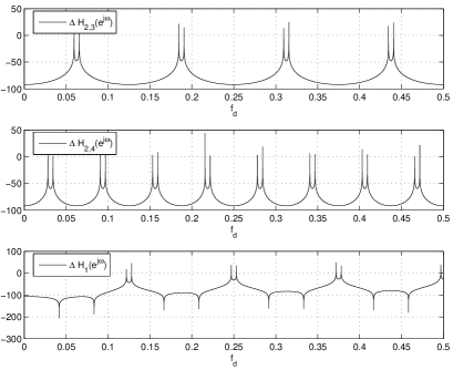
Figure 4: Frequency behaviours in dB of the functions $\left|\Delta H_{1}\left(e^{j\omega}\right)\right|$, $\left|\Delta H_{2,3}\left(e^{j\omega}\right)\right|$, and $\left|\Delta H_{2,4}\left(e^{j\omega}\right)\right|$ in (27) for $D=32,~{}D_{1}=8,~{}D_{2}=4$, $p_{p}=2$, $p=5$, $\nu=4$, $q=0.79$, and $\Delta h_{P}(n)=\Delta r_{i}=10^{-4},~{}\forall n,i$.

Some key observations are in order. Fig. 4 shows that the pass-band behaviour of the filter $H_{GCF_{3}}(e^{j\omega})$ is not affected by the approximation of its coefficients. Sensitivity of $H_{GCF_{3}}(e^{j\omega})$ is very low for $f_{d}\in\left[0,f_{c}\right]$, whereby $f_{c}=\frac{1}{2\rho}$. This in turn suggests that the filter pass-band droop does not degrade by virtue of multipliers’ approximations, and it is as low as the one guaranteed by filter $H_{GCF_{3}}(e^{j\omega})$. Notice also that the sensitivity is very low around the digital frequency $\frac{1}{D}-f_{c}$, which defines the selectivity of the decimation filter [1].

Fig.s 4 and 5 show that the approximation of multipliers $h_{P}(n)$ and $r_{u}$ affects the sensitivity of the frequency response $H_{GCF_{3}}(e^{j\omega})$ in disjoint folding bands. Indeed, filters $H_{P}(e^{j\omega})$ and $H_{N}(e^{j\omega})$ place the respective zeros in different digital frequencies, as clearly highlighted in Fig. 5.

Fig. 4 also shows that the frequency response $H_{GCF_{3}}(e^{j\omega})$ is very sensitive to coefficients’ approximations specially in the folding bands $\left[\frac{k}{D}-f_{c},\frac{k}{D}+f_{c}\right],~{}\forall k\in K_{k}$. This in turn suggests that particular care must be devoted to the approximation of multipliers embedded in both $H_{P}(z)$ and $H_{N}(z)$ in order to preserve the QN rejection performance around the folding bands. However, the same figure suggests that the approximation of the multipliers $r_{u}$s belonging to $H_{N}(z)$, can be done independently from the approximations of coefficients $h_{P}(n)$ belonging to $H_{P}(z)$.

Sensitivity analysis derived above, allows to draw a general picture of the effects of the approximations of the coefficients on the actual frequency response $\widetilde{H}_{GCF_{3}}(z)$. Nevertheless, we deduced that the sensitivity is very low in the pass-band $[0,f_{c}]$ and around the frequency $\frac{1}{D}-f_{c}$. This in turn suggests that both pass-band droop and selectivity of GCF filters are preserved by the approximations of the multipliers.

An important question is still open. We still need to quantify the extent of the effects of the coefficient approximations on the frequency response $\widetilde{H}_{GCF_{3}}(z)$. In brief, the basic question we want to answer is as follows. What are the approximation errors $\Delta r_{u},~{}\forall u=p_{p}+1,\ldots,p-1,$ and $\Delta h_{P}(n),~{}\forall n\in[0,3D_{1}-3],$ that we can tolerate on $\widetilde{H}_{GCF_{3}}(z)$? The answer to this question is the focus of the next section. It is anticipated that whatever the condition on the maximum approximation error tolerated on the frequency response $\widetilde{H}_{GCF_{3}}(e^{j\omega})$, it should be related to the behaviour of such a function around the folding bands, since both pass-band droop and selectivity of these filters are mainly unaffected by the approximation of the multipliers.

V Estimation of zero displacements due to coefficient approximations

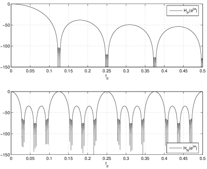
Figure 5: Frequency behaviours in dB of the functions $\left|H_{P}\left(e^{j\omega}\right)\right|$ and $\left|H_{N}\left(e^{j\omega}\right)\right|$, respectively, in (13) and (15) for $D=32,~{}D_{1}=8,~{}D_{2}=4$, $p_{p}=2$, $p=5$, $\nu=4$, $q=0.79$.

Besides improving the selectivity on the frequency $\frac{1}{D}-f_{c}$, GCF filters provide improved $\Sigma\Delta$ QN rejection around the folding bands with respect to classical, equal-order comb filters [9]. However, coefficient approximations can have detrimental effects on the zero locations in the $z$-plane, and, accordingly, can worsen $\Sigma\Delta$ QN rejection performance around the folding bands. As a consequence, it is useful to estimate the effects of coefficient approximations on the actual $\Sigma\Delta$ QN rejection performance guaranteed by filter $\widetilde{H}_{GCF_{3}}(e^{j\omega})$ by estimating the induced zero displacements. Next three sections address this topic by first examining filters $H_{P}(z)$ and $H_{N}(z)$ separately, and then deducing some hints from the derived theoretical analysis.

V-A Displacements of zeros belonging to $H_{P}(z)$

In this section, the focus is on the evaluation of the errors $\Delta z_{k}$ on the locations of the zeros of $H_{P}(z)$ due to the approximations of the coefficients $h_{P}(n)$ in the polyphase filter $H_{P}(e^{j\omega})$. First of all, notice that $H_{P}(z)$ places its $3\cdot D_{1}-3$ zeros in the following $z$ locations:

$$z_{k}=\left\{\begin{array}[]{ll}e^{+j2\pi\frac{k}{D_{1}}},&~{}\forall k=1,\ldots,\left\lfloor\frac{D_{1}}{2}\right\rfloor\\ e^{-j2\pi\frac{k}{D_{1}}},&~{}\forall k=1,\ldots,\left\lfloor\frac{D_{1}}{2}\right\rfloor-1\\ e^{+j2\pi\left(\frac{k}{D_{1}}+qf_{c}\right)},&~{}\forall k=1,\ldots,\left\lfloor\frac{D_{1}}{2}\right\rfloor-1\\ e^{-j2\pi\left(\frac{k}{D_{1}}+qf_{c}\right)},&~{}\forall k=1,\ldots,\left\lfloor\frac{D_{1}}{2}\right\rfloor-1\\ e^{\pm j2\pi\left(\frac{k}{D_{1}}-qf_{c}\right)},&~{}\forall k=1,\ldots,\left\lfloor\frac{D_{1}}{2}\right\rfloor\\ \end{array}\right.$$

The $z$-transfer function $H_{P}(z)$ in (13) can be expressed in a form emphasizing its zeros:

$$H_{P}(z)=\prod_{k=1}^{L-1}\left(1-z_{k}z^{-1}\right)$$ (28)

whereby $L=3\cdot D_{1}-2$. Due to the approximation of the coefficients $h_{P}(n)$, the set of zeros becomes $\{\widetilde{z}_{k}=z_{k}+\Delta z_{k},~{}\forall k=1,\ldots,L-1\}$:

$$\widetilde{H}_{P}(z)=\prod_{k=1}^{L-1}\left(1-\widetilde{z}_{k}z^{-1}\right)$$

Zero displacements $\Delta z_{k}$ can be related to the coefficient approximations $\Delta h_{P}$ as follows:

$$\Delta z_{i}=\sum_{\eta=1}^{L}\frac{\partial z_{i}}{\partial h_{P}(\eta)}\Delta h_{P}(\eta)$$ (29)

since there are $L$ coefficients $h_{P}(n)$ with $n\in[0,L-1]$.

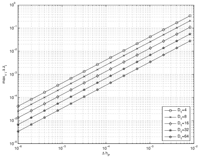
Figure 6: Maximum zero displacement over all the set of coefficients $h_{P}(n)$ as a function of the approximation error $\Delta h_{P}$. The results assume the same error $\Delta h_{P}$ for all the coefficients $h_{P}(n)$. Parameters are as follows: $D_{2}=4$, and $\nu=4$.

Upon noting that:

$$\frac{\partial H_{P}(z)}{\partial h_{P}(\eta)}_{|_{z=z_{i}}}=\frac{\partial H_{P}(z)}{\partial z}_{|_{z=z_{i}}}\cdot\frac{\partial z_{i}}{\partial h_{P}(\eta)}$$

it is straightforward to obtain:

$$\frac{\partial H_{P}(z)}{\partial h_{P}(\eta)}_{|_{z=z_{i}}}=-z^{-\eta}_{|_{z=z_{i}}}=-z_{i}^{-\eta}$$

by employing (13), and

$$\frac{\partial H_{P}(z)}{\partial z}_{|_{z=z_{i}}}=\left\{\sum_{k=1}^{L-1}\frac{z_{k}}{z^{2}}\prod_{l=1,l\neq k}^{L-1}\left(1-z_{l}z^{-1}\right)\right\}_{|_{z=z_{i}}}$$

by deriving (28) with respect to $z$. Finally, after some algebra (29) can be rewritten as follows:

$$\Delta z_{i}=-\sum_{\eta=1}^{L}\frac{z_{i}^{-\eta}\Delta h_{P}(\eta)}{\left\{\sum_{k=1}^{L-1}\frac{z_{k}}{z^{2}}\prod_{l=1,l\neq k}^{L-1}\left(1-z_{l}z^{-1}\right)\right\}_{|_{z=z_{i}}}}$$ (30)

which is the displacement of the $i$-th zero $z_{i}$ due to the approximations of all coefficients $h_{P}(n)$ belonging to the polyphase filter decimating by $D_{1}$.

Fig. 6 shows the maximum $\Delta z_{i}$ over all the set of zeros indexed by $i=1,\ldots,L$, as a function of the approximation error $\Delta h_{P}(\eta)=\Delta h_{P}$, assumed to be the same for all coefficients, for various values of $D_{1}$, $D_{2}=4$, and $\nu=4$. Curves shown in the figure can be considered as the worst case zero displacement due to the approximations of coefficients $h_{P}(n)$.

V-B Displacements of zeros belonging to $H_{N}(z)$

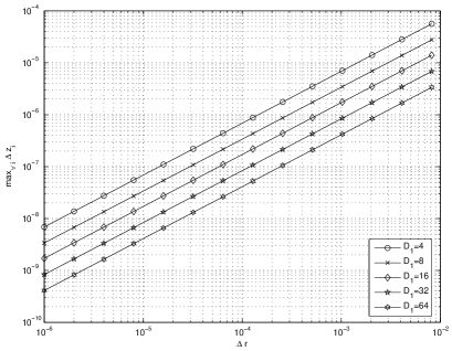
Figure 7: Maximum zero displacement over all the set of coefficients $r_{u}$ as a function of the approximation error $\Delta r$. Curves assume the same error $\Delta r$ for all the multipliers $r_{u}$. Parameters are as follows: $D_{2}=4$, and $\nu=4$.

In this section, the focus is on the evaluation of the displacements $\Delta z_{k}$ of the zeros in $H_{N}(z)$ due to the approximation of the coefficients $r_{u}$ belonging to $H_{N}(z)$. Error $\Delta z_{i}$ on the $i$-th zero can be related to the approximation errors of multipliers $r_{u}$s as follows:

$$\Delta z_{i}=\sum_{u=p_{p}+1}^{p-1}\frac{\partial z_{i}}{\partial r_{u}}\Delta r_{u}$$ (31)

Upon noting that:

$$\frac{\partial H_{N}(z)}{\partial r_{u}}_{|_{z=z_{i}}}=\frac{\partial H_{N}(z)}{\partial z}_{|_{z=z_{i}}}\cdot\frac{\partial z_{i}}{\partial r_{u}}$$

after some algebra on (10), it is possible to obtain:

$$\begin{array}[]{ll}\frac{\partial H_{N}(z)}{\partial r_{u}}_{|_{z=z_{i}}}=\left\{\left(z^{-2^{u}}+z^{-2\cdot 2^{u}}\right)\prod_{k=p_{p}+1,k\neq u}^{p-1}\left[1+\right.\right.\\ \left.\left.+r_{k}\left(z^{-2^{k}}+z^{-2\cdot 2^{k}}\right)+z^{-3\cdot 2^{k}}\right]\right\}_{|_{z=z_{i}}}\end{array}$$ (32)

By deriving (10) with respect to $z$, it is possible to write:

$$\begin{array}[]{ll}\frac{\partial H_{N}(z)}{\partial z}_{|_{z=z_{i}}}=\sum_{k=p_{p}+1}^{p-1}\left\{\left[r_{k}\left(2^{k}z^{-2^{k}-1}\right.\right.\right.&\\ \left.\left.\left.-2\cdot 2^{k}z^{-2\cdot 2^{k}-1}\right)-3\cdot 2^{k}z^{-3\cdot 2^{k}}\right]\cdot\right.&\\ \left.\prod_{l=p_{p}+1,l\neq k}^{p-1}\left[1+r_{l}\left(z^{-2^{l}}+z^{-2\cdot 2^{l}}\right)+z^{-3\cdot 2^{l}}\right]\right\}_{|_{z=z_{i}}}&\end{array}$$ (33)

Finally, (31) can be evaluated by substituting the ratio between (32) and (33) in place of $\frac{\partial z_{i}}{\partial r_{u}}$.

Fig. 7 shows the maximum $\Delta z_{i}$ over all the set of zeros belonging to $H_{N}(z)$, as a function of the approximation error $\Delta r_{u}=\Delta r$, assumed to be the same for all multipliers, for various values of $D_{1}$, $D_{2}=4$ and $\nu=4$.

A quick comparison between the results shown in Fig.s 6 and 7 reveals that the maximum zero displacement of the zeros belonging to $H_{N}(z)$ is much smaller than the one experienced by zeros belonging to $H_{P}(n)$. There are at least two basic reasons for such a behaviour. First, the number of multipliers $r_{u}$s is very small with respect to the number of coefficients $h_{P}(n)$ of the polyphase section. Secondly, any error $\Delta r_{u}$ slightly rotates the zeros belonging to the $u$-th decimation cell in $H_{N}(z)$ leaving them on the unit circle. This follows from the $z$-transfer function $\left[1+r_{u}\left(z^{-1}+z^{-2}\right)+z^{-3}\right]$ of the $u$-th decimation stage. On the other hand, approximation errors $\Delta h_{P}(n)$ can also move the zeros of $H_{P}(z)$ outside the unit circle in the $z$-plane worsening the $\Sigma\Delta$ QN rejection performance of the decimation filter.

The previous analysis suggests that the most critical filter in the partial polyphase architecture is the polyphase section $H_{P}(e^{j\omega})$. In order to deduce the maximum tolerable approximation error over the set of coefficients $\Delta h_{P}(n)$, the behaviour of filter $H_{P}(e^{j\omega})$ around the folding bands should be further investigated. This is the topic addressed in the next section.

V-C Design Considerations

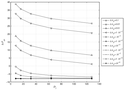
Figure 8: Behaviour of the difference $\Delta P_{qn}=\widetilde{P}_{{qn}|_{dB}}-P_{{qn}|_{dB}}$ as a function of the decimation factor $D_{1}$ and for various values of the approximation errors $\Delta h_{P}$ shown in the legend.

The $\Sigma\Delta$ QN power falling inside the folding bands $[\frac{k}{D_{1}}-f_{c},\frac{k}{D_{1}}+f_{c}],~{}\forall k=1,\ldots,\lfloor\frac{D_{1}}{2}\rfloor$, can be defined as [1]:

$$P_{qn}=\sum_{k=1}^{\lfloor\frac{D_{1}}{2}\rfloor}\int^{\frac{k}{D_{1}}+f_{c}}_{\frac{k}{D_{1}}-f_{c}}|H_{P}(e^{j\omega})|^{2}S_{B}(f_{d})df_{d}$$ (34)

where $S_{B}(f_{d})$, the power spectral density of the $\Sigma\Delta$ QN, can be expressed as $S_{B}(f_{d})=S_{e}(f_{d})\cdot[2\sin(\pi f_{d})]^{2B}$. In the previous relation $S_{e}(f_{d})=\frac{\Delta^{2}}{12f_{s}}$ is the power spectral density of the sampled noise under the hypothesis of representing the QN as a white noise [1], $\Delta$ is the quantization level of the quantizer contained in the $\Sigma\Delta$ modulator [1], and $f_{s}$ is the $\Sigma\Delta$ sampling rate.

In order to quantify the $\Sigma\Delta$ QN rejection performance of filter $\widetilde{H}_{P}(z)$ embedding the approximated multipliers $\widetilde{h}_{P}(n)=h_{P}(n)+\Delta h_{P}(n)$, with respect to a classical $3$rd order comb filter, the following performance metric, $\Delta P_{qn}$, can be evaluated:

$$\Delta P_{qn} =\frac{\sum_{k=1}^{\lfloor\frac{D_{1}}{2}\rfloor}\int^{\frac{k}{D}+f_{c}}_{\frac{k}{D}-f_{c}}|\widetilde{H}_{P}(f_{d})|^{2}S_{B}(f_{d})df_{d}}{\sum_{k=1}^{\lfloor\frac{D_{1}}{2}\rfloor}\int^{\frac{k}{D}+f_{c}}_{\frac{k}{D}-f_{c}}|H_{C_{3}}(f_{d})|^{2}S_{B}(f_{d})df_{d}}$$ (35)

The behaviour of $\Delta P_{qn}$-[dB] as a function of $D_{1}$ is shown in Fig. 8, for various values of $\Delta h_{P}$, i.e., the approximation error which is assumed to be the same for all the coefficients $h_{P}(n)$. Results in Fig. 8 show that $\Sigma\Delta$ QN rejection improvements can still be achieved upon approximating each coefficient $h_{P}(n)$ within an error less or equal to $10^{-3}$.

This in turn suggests that it is possible to optimize each multiplier $h_{P}(n)$ in the polyphase filter $H_{P}(z)$ by approximating it as a power-of-2 (PO2) coefficient with an approximation error of $10^{-3}$ without affecting the $\Sigma\Delta$ QN rejection performance of the polyphase filter around the folding bands for any $D_{1}\geq 32$.

Fig. 9 shows the behaviours of both the frequency response of filter $H^{*}_{GCF_{3}}(e^{j\omega})$ employing approximated coefficients $\widetilde{h}_{P}(n)=h_{P}(n)+\Delta h_{P}(n)$, and the frequency response of filter $H_{GCF_{3}}(e^{j\omega})$ embedding the real coefficients $h_{P}(n)$, for $D=D_{1}=64$, $\nu=4$, and $\Delta h_{P}(n)=\Delta h_{P}=10^{-3},~{}\forall n$. This is the most critical case in which a full polyphase architecture is employed. The lower subplot shows the local behaviour of both frequency responses around some folding bands. Notice that both curves are superimposed, even though $H^{*}_{GCF_{3}}(e^{j\omega})$ employs coefficients approximated with an error equal to $10^{-3}$.

The approximation of the multipliers $h_{P}(n)$ with PO2 coefficients is beyond the scope of this work. Nevertheless, many excellent works have been proposed in literature for obtaining the best PO2 coefficient approximation within a predefined error. We invite the interested readers to refer to papers [17]-[19].

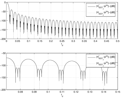
Figure 9: Modulo of the frequency response of filter $H^{*}_{GCF_{3}}(e^{j\omega})$ employing approximated coefficients $\widetilde{h}_{P}(n)=h_{P}(n)+\Delta h_{P}(n)$ (continuous curve), and frequency response of filter $H_{GCF_{3}}(e^{j\omega})$ embedding the real coefficients $h_{P}(n)$, for $D=D_{1}=64$, $\nu=4$, and $\Delta h_{P}(n)=\Delta h_{P}=10^{-3},~{}\forall n$. Lower subplot shows the behaviours of such functions around five folding bands.

Let us summarize the main design considerations deduced from the proposed sensitivity analysis of partial polyphase GCF filters.

• Both pass-band droop and selectivity performance of GCF filters are mainly unaffected by the approximation of the multipliers embedded in the decimation filter. Practically speaking, this means that such performance are the one already deduced in the companion paper [9].

• The most critical section in the partial polyphase decomposition is the polyphase filter $H_{P}(z)$.

• Upon approximating each multiplier of the polyphase section with an approximation error less or equal to $10^{-3}$, it is possible to preserve the $\Sigma\Delta$ QN rejection performance of GCF filters with respect to classical, equal-order comb filters, for a wide range of decimation factors $D_{1}$ as noted in the abscissa of Fig. 8.

VI Conclusions

This paper focused on the design of generalized comb filters by proposing a novel partial polyphase architecture with the aim to reduce the data rate after the $\Sigma\Delta$ A/D conversion. We proposed a mathematical framework in order to analyze both the sensitivity of the frequency response and the displacements of the zeros in the filter transfer functions due to the quantization of the multipliers embedded in the proposed filters.

We also derived the impulse response of a $3$rd order sample GCF filter, that we used as a reference scheme throughout the paper.

Appendix

In this Appendix, we derive the impulse response $h_{GCF_{3}}(n),~{}\forall n=0,\ldots,3D-3,$ of a $3$rd-order GCF filter decimating by $D$. The proof relies on repeated applications of the inverse $z$-transform on the product of two analytical functions $X_{1}(z)$ and $X_{2}(z)$ related to two discrete-time sequences, $x_{1}(n)$ and $x_{2}(n)$:

$$\begin{array}[]{ll}Z^{-1}\left[X_{1}(z)X_{2}(z)\right]=x_{1}(n)\star x_{2}(n)=&\\ =\sum_{k=-\infty}^{+\infty}x_{1}(k)x_{2}(n-k).&\end{array}$$ (36)

First of all, consider the transfer function in (5), and define as $X_{t}(z)$ the numerator $z$-polynomial:

$$\begin{array}[]{ll}X_{t}(z)=\left(1-z^{-D}e^{j\alpha D}\right)\left(1-z^{-D}e^{-j\alpha D}\right)\left(1-z^{-D}\right)&\\ =\left[1-rz^{-D}+rz^{-2D}-z^{-3D}\right]&\end{array}$$

whereby $r=1+2\cos(\alpha D)$. The discrete-time, causal sequence with $z$-transfer function $X_{t}(z)$ can be written as follows:

$$x_{t}(n)=\delta(n)-r\delta(n-D)+r\delta(n-2D)-\delta(n-3D)$$ (37)

whereby $\delta(n)$ is the discrete-time unit impulse centered in $n=0$.

Let us define the following pairs of transfer functions along with the respective discrete-time sequences [16]:

$$\begin{array}[]{lll}Y_{1}(z)=\frac{1}{1-z^{-1}}&\longleftrightarrow&y_{1}(n)=u(n)\\ Y_{2}(z)=\frac{1}{1-z^{-1}e^{-j\alpha}}&\longleftrightarrow&y_{2}(n)=e^{-j\alpha}u(n)\\ Y_{3}(z)=\frac{1}{1-z^{-1}e^{j\alpha}}&\longleftrightarrow&y_{3}(n)=e^{+j\alpha}u(n)\end{array}$$

whereby $u(n)$ is the discrete-time unitary-step sequence.

With the setup above, $H_{GCF_{3}}(z)$ in (5) can be rewritten as follows:

$$H_{GCF_{3}}(z)=X_{t}(z)\cdot Y_{1}(z)\cdot Y_{2}(z)\cdot Y_{3}(z)$$

Upon applying (36) to the $z$-function $W_{1}(z)=X_{t}(z)Y_{1}(z)$, it is possible to obtain:

$$w_{1}(n)=\sum_{k_{1}=-\infty}^{+\infty}x_{t}(k_{1})y_{1}(n-k_{1})$$ (38)

Applying (36) to the $z$-function $W_{2}(z)=W_{1}(z)Y_{2}(z)$, and employing (38), it is possible to obtain:

$$\begin{array}[]{ll}w_{2}(n)=\sum_{k_{2}=-\infty}^{+\infty}w_{1}(k_{2})y_{2}(n-k_{2})=&\\ =\sum_{k_{2}=-\infty}^{+\infty}\sum_{k_{1}=-\infty}^{+\infty}x_{t}(k_{1})y_{1}(k_{2}-k_{1})y_{2}(n-k_{2})&\end{array}$$ (39)

Finally, applying (36) to the $z$-function $H_{GCF_{3}}(z)=W_{3}(z)=W_{2}(z)Y_{3}(z)$, and employing (39), it is possible to obtain:

$$h_{GCF_{3}}(n)=\sum_{k_{3}=-\infty}^{+\infty}w_{2}(k_{3})y_{3}(n-k_{3})=$$

$$=\sum_{k_{3}=-\infty}^{+\infty}\sum_{k_{2}=-\infty}^{+\infty}\sum_{k_{1}=-\infty}^{+\infty}\left[x_{t}(k_{1})y_{1}(k_{2}-k_{1})\cdot\right.$$

$$\left.\cdot y_{2}(k_{3}-k_{2})y_{3}(n-k_{3})\right]$$ (40)

Upon substituting the respective expressions of the sequences $y_{i}(n),~{}\forall i=1,\ldots,3$ in (38), it is possible to write:

$$h_{GCF_{3}}(n)=\sum_{k_{3}=-\infty}^{+\infty}\sum_{k_{2}=-\infty}^{+\infty}\sum_{k_{1}=-\infty}^{+\infty}\left[x_{t}(k_{1})u(k_{2}-k_{1})\cdot\right.$$

$$\left.\cdot e^{-j\alpha(k_{3}-k_{2})}u(k_{3}-k_{2})e^{+j\alpha(n-k_{3})}u(n-k_{3})\right]$$ (41)

By exploiting the definitions of the unitary-step sequences, it is possible to observe the following relations:

$$u(k_{2}-k_{1})=\left\{\begin{array}[]{ll}1&~{}\forall k_{2}\geq k_{1}\\ 0&~{}\forall k_{2}<k_{1}\end{array}\right.$$

$$u(k_{3}-k_{2})=\left\{\begin{array}[]{ll}1&~{}\forall k_{3}\geq k_{2}\\ 0&~{}\forall k_{3}<k_{2}\end{array}\right.$$

$$u(n-k_{3})=\left\{\begin{array}[]{ll}1&~{}\forall n\geq k_{3}\\ 0&~{}\forall n<k_{3}\end{array}\right.$$

Based on these observations, we can reduce the upper limits of the summations in (Appendix) as follows:

$$h_{GCF_{3}}(n)=\sum_{k_{3}=-\infty}^{n}\sum_{k_{2}=-\infty}^{k_{3}}\sum_{k_{1}=-\infty}^{k_{2}}\left[x_{t}(k_{1})\cdot\right.$$

$$\left.\cdot e^{-j\alpha(k_{3}-k_{2})}e^{+j\alpha(n-k_{3})}\right]$$ (42)

By observing that the sequence $x_{t}(k_{1})$ is causal (see (37)), i.e., $x_{t}(k_{1})=0,~{}\forall k_{1}<0$, it is possible to obtain:

$$h_{GCF_{3}}(n)=e^{+j\alpha n}\sum_{k_{3}=0}^{n}e^{-2j\alpha k_{3}}\sum_{k_{2}=0}^{k_{3}}e^{j\alpha k_{2}}\sum_{k_{1}=0}^{k_{2}}x_{t}(k_{1})$$ (43)

Notice that the impulse response $h_{GCF_{3}}(n)$ generalizes the one of the classical $3$rd order comb decimation filter, and, it is composed by $3D-2$ coefficients over the time interval ranging from $0$ to $3D-3$. Equ. (43) can also be used as an on-line algorithm for generating the coefficients of the GCF impulse response $h_{GCF_{3}}(n)$ by simply solving the three nested summations for each $n=0,\ldots,3D-3$.

As a note aside, notice that by imposing $\alpha=0$ in (43), it is possible to obtain the impulse response of a classical $3$rd-order comb filter.

References

- [1] S. R. Norsworthy, R. Schreier, and G. C. Temes, Delta-Sigma Data Converters, Theory, Design, and Simulation, IEEE Press, 1997.
- [2] E. B. Hogenauer, “An economical class of digital filters for decimation and interpolation,” IEEE Trans. on Ac., Speech and Sign. Proc., Vol. ASSP-29, pp. 155-162, No. 2, April 1981.
- [3] J.C. Candy, “Decimation for sigma delta modulation,” IEEE Trans. on Comm., Vol. COM-34, pp.72-76, No. 1, January 1986.
- [4] R. E. Crochiere and L. R. Rabiner, Multirate Digital Signal Processing, Prentice-Hall PTR, 1983.
- [5] S. Chu and C. S. Burrus, “Multirate filter designs using comb filters,” IEEE Transactions on Circuits and Systems, vol. CAS-31, pp. 913 924, Nov. 1984.
- [6] L. Lo Presti, “Efficient modified-sinc filters for sigma-delta A/D converters,” IEEE Trans. on Circ. and Syst.-II, Vol. 47, pp. 1204-1213, No. 11, November 2000.
- [7] M. Laddomada, L. Lo Presti, M. Mondin, and C. Ricchiuto, ”An efficient decimation sinc–filter design for software radio applications”, In Proc. of IEEE SPAWC, March 20-23, 2001.
- [8] L. Lo Presti and A. Akhdar, “Efficient antialising decimation filter for converters,” In Proc. of ICECS98, Vol.1, pp. 367-370, Sept. 1998.
- [9] M. Laddomada, “Generalized comb decimation filters for A/D converters: Analysis and design,” IEEE Trans. on Circuits and Systems I, Vol.54, No. 5, pp. 994-1005, May 2007.
- [10] Y. Gao, J. Tenhunen, and H. Tenhunen, “A fifth-order comb decimation filter for multi-standard transceiver applications,” In Proceedings of ISCAS 2000, IEEE International Symposium on Circuits and Systems, May 28-31, 2000, Geneva, Switzerland, pp. III-89-III-92.
- [11] H. Aboushady, Y. Dumonteix, M. Lourat, and H. Mehrez, “Efficient polyphase decomposition of comb decimation filters in analog-to-digital converters,” IEEE Trans. on Circ. and Syst.-II, Vol. 48, pp. 898-903, No. 10, October 2001.
- [12] A.Y. Kwentus, Z. Jiang, and A.N. Willson Jr., “Application of filter sharpening to cascaded integrator-comb decimation filters,” IEEE Trans. on Signal Proc., Vol. 45, pp. 457-467, No. 2, February 1997.
- [13] G. Jovanovic-Dolecek and S.K. Mitra, “A new two-stage sharpened comb decimator,” IEEE Trans. on Circ. and Syst.-I, Vol. 52, pp. 1414-1420, No. 7, July 2005.
- [14] M. Laddomada and M. Mondin, “Decimation schemes for A/D converters based on Kaiser and Hamming sharpened filters,” IEE Proceedings of Vision, Image and Signal Processing, Vol. 151, No. 4, pp. 287-296, August 2004.
- [15] M. Laddomada, “Comb-based decimation filters for A/D converters: Novel schemes and comparisons,” IEEE Trans. on Signal Processing, Vol.55, No. 5, Part 1, pp. 1769-1779, May 2007.
- [16] A. Antoniou, Digital Signal Processing: Signals, Systems, and Filters, McGraw-Hill, 2005, ISBN 0-07-145425-X.
- [17] Y.C. Lim and S.R. Parker, “FIR filter design over a discrete powers-of-two coefficient space,” IEEE Trans. on ASSP, vol. ASSP-31, No. 3, pp. 583 -591, June 1983.
- [18] W.J. Oh and Y.H. Lee, “Implementation of programmable multiplierless FIR filters with powers-of-two coefficients,” IEEE Trans. on Circuits and Systems II, vol. 42, No. 8, pp. 553 -556, August 1995.
- [19] D. Li, Y.C. Lim, Y. Lian, and J. Song, “A polynomial-time algorithm for designing FIR filters with powers-of-two coefficients,” IEEE Trans. on Signal Proc., vol. 50, No. 8, pp. 1935 -1941, August 2002.