Effective mean-field equations for cigar-shaped and disk-shaped Bose-Einstein condensates

Abstract

By applying the standard adiabatic approximation and using the accurate analytical expression for the corresponding local chemical potential obtained in our previous work [Phys. Rev. A 75, 063610 (2007)] we derive an effective 1D equation that governs the axial dynamics of mean-field cigar-shaped condensates with repulsive interatomic interactions, accounting accurately for the contribution from the transverse degrees of freedom. This equation, which is more simple than previous proposals, is also more accurate. Moreover, it allows treating condensates containing an axisymmetric vortex with no additional cost. Our effective equation also has the correct limit in both the quasi-1D mean-field regime and the Thomas-Fermi regime and permits one to derive fully analytical expressions for ground-state properties such as the chemical potential, axial length, axial density profile, and local sound velocity. These analytical expressions remain valid and accurate in between the above two extreme regimes. Following the same procedure we also derive an effective 2D equation that governs the transverse dynamics of mean-field disk-shaped condensates. This equation, which also has the correct limit in both the quasi-2D and the Thomas-Fermi regime, is again more simple and accurate than previous proposals. We have checked the validity of our equations by numerically solving the full 3D Gross-Pitaevskii equation.

I I. INTRODUCTION

The experimental realization of Bose-Einstein condensates (BECs) of dilute atomic gases confined in optical and magnetic traps BEC1 ; BEC2 ; BEC3 has opened new opportunities for investigating the coherence properties of degenerate quantum systems. From a theoretical point of view, under the usual experimental conditions these systems can be accurately described by the Gross-Pitaevskii equation (GPE) GPE , a mean-field equation of motion governing the behavior of the condensate wave function $\psi(\mathbf{r},t)$

$$i\hbar\frac{\partial\psi}{\partial t}=\left(-\frac{\hbar^{2}}{2m}\nabla^{2}+V(\mathbf{r})+gN\left|\psi\right|^{2}\right)\psi.$$ (1)

In the above equation $N$ is the number of atoms, $g=4\pi\hbar^{2}a/m$ is the interaction strength, $a$ is the s-wave scattering length, and $V(\mathbf{r})$ is the potential of the confining trap. In what follows we shall restrict ourselves to the usual case of condensates with repulsive interatomic interactions ($a>0$).

The GPE has proved to be very successful in describing the evolution in time of dilute quantum gases near the zero-temperature limit. From a mathematical point of view this equation is a time-dependent nonlinear differential equation. Since no explicit analytical solutions are known, in general, Eq. (1) has to be solved numerically. This is a nontrivial numerical task that demands a considerable computational effort. Moreover, in many circumstances the superfluid dynamics of a zero-temperature condensate can become chaotic which requires large basis or grid point sets to guarantee convergence PRL06 . In recent years there has been particular interest in BECs confined in highly anisotropic traps Olsha1 ; Petrov1 ; Petrov2 ; Dunj1 ; Das1 ; Kett1 ; Strin1 . In such geometries the condensate is so tightly confined in the radial or the axial dimension that the corresponding dynamics becomes effectively one dimensional or two dimensional, respectively. The time evolution of these systems with reduced dimensionality is characterized by two very different time scales. Even though usually one is only interested in the evolution of the slow degrees of freedom in the effective mean field induced by the fast degrees of freedom, from a computational point of view it is also required to resolve accurately the irrelevant fast degrees of freedom. It is clear that for sufficiently anisotropic traps this can represent a computational challenge. It is therefore convenient to develop theoretical models that permit one to study the condensate dynamics in terms of effective equations of lower dimensionality. In this regard various approaches have been followed in recent years Jack1 ; Chio1 ; Reatto1 ; Modug1 ; Kam1 ; You1 . Among them, the effective 1D and 2D nonpolynomial nonlinear Schrödinger equations by Salasnich et al. Reatto1 have proved the most efficient.

In this work we derive effective 1D and 2D wave equations that govern the dynamics of mean-field cigar-shaped and disk-shaped condensates with repulsive interatomic interactions. These equations which incorporate properly the contribution from the fast degrees of freedom have the correct limits in both the TF and the perturbative regime. Even though the equations by Salasnich et al. are in general very accurate, we demonstrate that our effective equations are more accurate. Moreover, as a consequence of its simplicity, they also permit one to obtain fully analytical expressions for various relevant ground-state properties such as chemical potentials, condensate lengths, density profiles, and local sound velocities.

II II. CIGAR-SHAPED CONDENSATES

Consider a BEC confined in a highly elongated trap. The high anisotropy of the trap has important consequences on the condensate dynamics which under usual conditions becomes governed by two very different time scales. In these circumstances the characteristic evolution time of the fast transverse motion ($\sim\omega_{\bot}^{-1}$) is so small in comparison with the characteristic time scale of the axial motion ($\sim\omega_{z}^{-1}$) that one can assume that at every instant of time the transverse degrees of freedom adjust instantaneously to the lowest-energy configuration compatible with the axial configuration occurring at that time (adiabatic approximation). This implies, in particular, that the correlations between transverse and axial motions can be neglected and the condensate wave function can be factorized as Jack1 ; Kramer1

$$\psi(\mathbf{r},t)=\varphi(\mathbf{r}_{\bot};n_{1}(z,t))\phi(z,t),$$ (2)

where $\mathbf{r}_{\bot}=(x,y)$ and $n_{1}(z,t)$ is the local condensate density per unit length characterizing the axial configuration

$$n_{1}(z,t)\equiv N\int d^{2}\mathbf{r}_{\bot}|\psi(\mathbf{r}_{\bot},z,t)|^{2}.$$ (3)

Normalizing the transverse wave function to unity

$$\int d^{2}\mathbf{r}_{\bot}|\varphi(\mathbf{r}_{\bot};n_{1})|^{2}=1,$$ (4)

Eq. (3) takes the desirable form

$$n_{1}(z,t)=N|\phi(z,t)|^{2}.$$ (5)

Substituting now the wave function (2) into the GPE and assuming the confining potential to be separable as $V(\mathbf{r})=V_{\bot}(\mathbf{r}_{\bot})+V_{z}(z)$, one obtains

$$\left(i\hbar\frac{\partial\phi}{\partial t}+\frac{\hbar^{2}}{2m}\frac{\partial^{2}\phi}{\partial z^{2}}-V_{z}(z)\phi\right)\varphi(\mathbf{r}_{\bot};n_{1})=\\ \left(-\frac{\hbar^{2}}{2m}\nabla_{\bot}^{2}\varphi+V_{\bot}(\mathbf{r}_{\bot})\varphi+gn_{1}(z,t)\left|\varphi\right|^{2}\varphi\right)\phi(z,t).$$ (6)

Both the axial and time variations induced in the transverse wave function $\varphi$ by the axial density $n_{1}$ have been neglected in the above equation. Neglecting the time derivative of $\varphi$ is in fact the essence of the adiabatic approximation already discussed. Neglecting the second derivative of $\varphi$ with respect to $z$ requires the axial density to vary sufficiently slowly along the axial direction. For condensates in highly elongated traps such condition usually holds in most cases of practical interest.

Multiplying Eq. (6) by $\varphi^{\ast}(\mathbf{r}_{\bot};n_{1})$ and integrating on the transverse coordinates $\mathbf{r}_{\bot}$ we arrive at

$$i\hbar\frac{\partial\phi}{\partial t}=-\frac{\hbar^{2}}{2m}\frac{\partial^{2}\phi}{\partial z^{2}}+V_{z}(z)\phi+\mu_{\bot}(n_{1})\phi,$$ (7)

where we have defined

$$\mu_{\bot}(n_{1})\!\equiv\!\!\int\!d^{2}\mathbf{r}_{\bot}\varphi^{\ast}\!\left(\!-\frac{\hbar^{2}}{2m}\nabla_{\bot}^{2}+V_{\bot}(\mathbf{r}_{\bot})+gn_{1}\left|\varphi\right|^{2}\!\right)\!\varphi.$$ (8)

Equation (7) is an effective 1D mean-field equation that governs the axial dynamics of cigar-shaped BECs, incorporating the contribution from the transverse degrees of freedom through $\mu_{\bot}(n_{1})$. Substitution of Eq. (7) into Eq. (6) yields

$$\left(-\frac{\hbar^{2}}{2m}\nabla_{\bot}^{2}+V_{\bot}(\mathbf{r}_{\bot})+gn_{1}\left|\varphi\right|^{2}\right)\varphi=\mu_{\bot}(n_{1})\varphi,$$ (9)

which shows that at every instant of time and $z$ plane the transverse wave function $\varphi$ satisfies the stationary GPE of an axially homogeneous condensate characterized by a density per unit length $n_{1}(z,t)$, with $\mu_{\bot}(n_{1})$ being the corresponding (transverse) local chemical potential. Clearly, the usefulness of the effective 1D axial equation (7) depends, to a great extent, on the possibility of finding a simple way of solving Eq. (9). In this regard, it is important to note that $n_{1}$ enters the equation above as a mere external parameter, so that, in practice, the solution of the transverse equation does not require the knowledge of the axial evolution. Before considering this problem in more detail we will first take a look at the condensate stationary states, which must satisfy

$$\phi(z,t)=\phi_{0}(z)e^{-i\mu t/\hbar}.$$ (10)

Substituting in Eq. (7) one obtains

$$-\frac{\hbar^{2}}{2m}\frac{\partial^{2}\phi_{0}}{\partial z^{2}}+V_{z}(z)\phi_{0}+\mu_{\bot}(n_{1})\phi_{0}=\mu\phi_{0},$$ (11)

where the condensate chemical potential$\ \mu$ is the Lagrange parameter that guarantees the normalization condition $\int dz|\phi(z,t)|^{2}=1$. When $\phi_{0}$ varies so slowly that the typical length scale $\Delta_{z}$ of its spatial variations along $z$ is much greater than the corresponding axial healing length, i.e.,

$$\Delta_{z}\gg\frac{\hbar}{\sqrt{2m(\mu_{\bot}(n_{1})-\hbar\omega_{\bot})}},$$ (12)

then the first term on the left in Eq. (11) can be neglected in comparison with the mean-field interaction energy and one arrives at the local density approximation

$$\mu=\mu_{\bot}(n_{1})+V_{z}(z).$$ (13)

When this equation is applicable, the knowledge of the transverse chemical potential permits one to obtain an analytic expression for the ground-state axial condensate profile $n_{1}(z)$. In any case, as Eq. (7) shows, the analytic determination of $\mu_{\bot}(n_{1})$ is the key ingredient to derive a useful 1D effective equation of motion for the condensate axial dynamics.

We shall concentrate in what follows on cigar-shaped condensates confined in the radial direction by an axisymmetric harmonic potential characterized by an oscillator length $a_{\bot}=\sqrt{\hbar/m\omega_{\bot}}$,

$$V(\mathbf{r})=\frac{1}{2}m\omega_{\bot}^{2}r_{\bot}^{2}+V_{z}(z).$$ (14)

Introducing dimensionless variables $\overline{r}_{\bot}=r_{\bot}/a_{\bot}$ and $\overline{\varphi}=a_{\bot}\varphi$, the transverse equation (9) determining the local chemical potential $\overline{\mu}_{\bot}=\mu_{\bot}/\hbar\omega_{\bot}$ takes the form Strin1

$$\left(-\frac{1}{2}\overline{\nabla}_{\bot}^{2}+\frac{1}{2}\overline{r}_{\bot}^{2}+4\pi an_{1}\left|\overline{\varphi}\right|^{2}\right)\overline{\varphi}=\overline{\mu}_{\bot}(n_{1})\overline{\varphi}.$$ (15)

This equation, that depends on the sole parameter $an_{1}$, can be analytically solved in two limiting cases. When $an_{1}\ll 1$ the mean-field interaction energy can be treated as a weak perturbation. In this perturbative regime the condensate wave function that minimizes the energy functional is given, to the lowest order, by the Gaussian ground state of the harmonic oscillator and the condensate is tightly confined in the radial direction. Under these conditions the radial motion is frozen out, restricted to zero-point oscillations, and the condensate becomes effectively one dimensional. Thus the perturbative regime corresponds to quasi-1D mean-field condensates with a local chemical potential given by

$$\overline{\mu}_{\bot}(n_{1})=1+2an_{1}.$$ (16)

When $an_{1}\gg 1$ the kinetic energy term can be safely neglected in comparison with the mean-field interaction energy. This is the Thomas-Fermi regime, in which many modes of the transverse harmonic trap become excited and the condensate exhibits a parabolic radial profile

$$\left|\overline{\varphi}\right|^{2}=\frac{1}{4\pi an_{1}}\left(\overline{\mu}_{\bot}-\frac{1}{2}\overline{r}_{\bot}^{2}\right),$$ (17)

where the local chemical potential ensuring normalization is now given by

$$\overline{\mu}_{\bot}(n_{1})=2\sqrt{an_{1}}.$$ (18)

Note that in passing from the Thomas-Fermi regime to the perturbative regime the system undergoes an effective dimensional crossover from a 3D cigar-shaped condensate to a quasi-1D mean-field condensate.

In previous works Previos , by using a suitable approximation scheme, we derived general approximate formulas that provide with remarkable accuracy (typically better than $1\%$) the ground-state properties of any mean-field scalar Bose-Einstein condensate with short-range repulsive interatomic interactions, confined in arbitrary cylindrically symmetric harmonic traps, and even containing a multiply quantized axisymmetric vortex. This approximation scheme essentially represents an extension of the Thomas-Fermi approximation that incorporates conveniently the zero-point energy contribution. In the limiting cases of cigar-shaped and disk-shaped condensates the ground-state properties follow from explicit analytical formulas that reduce to the correct analytical expressions in both the TF and the perturbative regimes, and remain valid and accurate in between these two limiting cases, thus accounting properly for the corresponding dimensional crossover. Physical quantities such as the condensate radius, axial length, chemical potential, mean-field interaction energy, kinetic and potential energies, density profiles, and local sound velocities can be easily and accurately obtained in this way in terms of the physically relevant parameters (number of atoms, trap aspect ratio, and vortex charge). In particular, in Ref. Previos , we found that the transverse local chemical potential of a condensate with an axisymmetric vortex of charge $q$, as a function of the condensate density per unit length $n_{1}$, is given by

$$\overline{\mu}_{\bot}(n_{1})=(|q|+1)+\sqrt{\beta_{q}^{2}+4an_{1}}-\beta_{q},$$ (19)

with

$$\beta_{q}=\frac{2^{2|q|}(|q|!)^{2}}{(2|q|)!}.$$ (20)

The parameter $\beta_{q}^{-1}$ accounts for the dilution effect that the centrifugal force associated with the vortex has on the condensate mean density Previos . In the absence of vortices $q=0\rightarrow\beta_{q}=1$, the equation above simplifies to

$$\overline{\mu}_{\bot}(n_{1})=\sqrt{1+4an_{1}}.$$ (21)

Clearly, in the appropriate limits, this equation reduces to the quasi-1D and TF expressions (16) and (18), respectively. As we shall see, it also describes correctly the corresponding dimensional crossover.

The above equations were derived in Ref. Previos by using a suitable TF-like ansatz for the local density $\left|\psi(r_{\bot},z)\right|^{2}$ of a harmonically trapped BEC in its ground state. Such local density, which is not factorizable in general, is defined in a volume that corresponds to the usual TF ellipsoidal density cloud conveniently truncated in order to account for the zero-point energy contribution. Note that even though the expression (19) was originally obtained for a condensate in its ground state (compatible with an axisymmetric vortex of charge $q$) and axially confined by a harmonic potential, it is, however, of general validity. This is so because, as already said, the solution of the transverse equation (15) does not depend on the particular axial evolution. To convince the reader that this is the case we have numerically solved Eq. (15) for a wave function of the form

$$\overline{\varphi}(\overline{\mathbf{r}}_{\bot})=\exp(iq\theta)\overline{\varphi}_{q}(\overline{r}_{\bot}),$$ (22)

with $q=0,1,2,$ and $4$. The results of the numerical calculation are shown in Fig. 1 (open circles) along with the theoretical prediction obtained from Eq. (19) (solid lines). As is apparent, Eq. (19) accurately accounts for the dimensional crossover, the agreement with the numerical results being excellent for any value of the dimensionless interaction parameter $an_{1}$. The maximum error is smaller than $1\%$ for $q=0$ and $2$, and smaller than $1.2\%$ for $q=1$. Even though one expects Previos this maximum error to increase with $q$, it is still smaller than $2.5\%$ for $q=4$. This demonstrates that the local chemical potential as given by Eq. (19) is an accurate solution of the transverse equation (9). This result is of interest in its own right. For instance, in Ref. Kramer1 , it has been shown that the velocity of sound in an axially uniform Bose-Einstein condensate immersed in a 1D optical lattice and radially confined by a harmonic trap can be obtained, in a wide range of optical lattice depths, from the knowledge of the local chemical potential $\overline{\mu}_{\bot}$ as a function of the linear average density $n_{1}=N/d$, with $d$ being the lattice period. In such an approach the effect of the lattice is incorporated into a suitable renormalization of the mass and of the coupling constant. In the present work, however, the main interest of Eq. (19) comes from the fact that when substituted in Eq. (7) it leads to the following effective 1D mean-field equation:

Figure 1: (Color online) Theoretical prediction for the transverse local chemical potential $\overline{\mu}_{\bot}$ as a function of $an_{1}$ for different vortex charges $q$ (solid lines). The open circles are exact numerical results obtained by solving the stationary Gross-Pitaevskii equation (15).

$$i\hbar\frac{\partial\phi}{\partial t}=-\frac{\hbar^{2}}{2m}\frac{\partial^{2}\phi}{\partial z^{2}}+V_{z}(z)\phi+\hbar\omega_{\bot}\sqrt{\beta_{q}^{2}+4aN\left|\phi\right|^{2}}\phi,$$ (23)

where $\beta_{q}$ is given by Eq. (20) and we have absorbed the constant term proportional to $(|q|+1)-\beta_{q}$ into the definition of the generic axial potential $V_{z}(z)$. For $q=0,1,2,...$ the parameter $\beta_{q}$ takes the values $1,2,8/3,...$, respectively.

Equation (23) is the equation we were looking for. It governs the axial dynamics of arbitrary mean-field cigar-shaped condensates with repulsive interatomic interactions even in the presence of an axisymmetric vortex of charge $q$, accounting for the effects from the transverse degrees of freedom through the term proportional to $\hbar\omega_{\bot}$. Since vortices with $q\geq 2$ are dynamically unstable and decay into an array of singly quantized vortices PRL06 ; Mott , in such cases the applicability of Eq. (23) is restricted to times shorter than the corresponding decay time. As is apparent, the equation above is much simpler than previous proposals. It is also more accurate, as we shall see. Since we have found an expression for the transverse local chemical potential that is very accurate, the validity of Eq. (23) relies almost exclusively on the validity of the well established adiabatic approximation.

When $4an_{1}\ll\beta_{q}^{2}$ one enters the quasi-1D mean-field regime. In this case, Eq. (23) reduces to

$$i\hbar\frac{\partial\phi}{\partial t}=-\frac{\hbar^{2}}{2m}\frac{\partial^{2}\phi}{\partial z^{2}}+V_{z}(z)\phi+g_{\mathrm{1D}}N\left|\phi\right|^{2}\phi,$$ (24)

with

$$g_{\mathrm{1D}}=\beta_{q}^{-1}\frac{g}{2\pi a_{\bot}^{2}}=\beta_{q}^{-1}2a\hbar\omega_{\bot}.$$ (25)

This equation generalizes the well-known 1D GPE to the case of condensates containing an axisymmetric vortex. In the absence of vortices, $\beta_{q}=1$ and one recovers the usual equation. When the number of particles is high enough that $4an_{1}\gg\beta_{q}^{2}$, the condensate enters the TF regime. In this case, Eq. (23) reduces to

$$i\hbar\frac{\partial\phi}{\partial t}=-\frac{\hbar^{2}}{2m}\frac{\partial^{2}\phi}{\partial z^{2}}+V_{z}(z)\phi+2\hbar\omega_{\bot}\sqrt{aN}\left|\phi\right|\phi,$$ (26)

which again is the correct result as follows from the direct substitution of Eq. (18) into Eq. (7).

The effective 1D equation (23) also permits deriving an accurate analytical expression for the stationary axial density profile $n_{1}(z)=N|\phi_{0}(z)|^{2}$. To see this we shall consider a harmonic axial confinement $V_{z}(z)=\frac{1}{2}m\omega_{z}^{2}z^{2}$ with corresponding oscillator length $a_{z}=\sqrt{\hbar/m\omega_{z}}$. For cigar-shaped condensates the trap aspect ratio $\lambda=\omega_{z}/\omega_{\bot}$ must satisfy the inequality $\lambda\ll 1$. Under these circumstances the condition (12) can be easily fulfilled. It would be sufficient (though not necessary) that $\Delta_{z}\gg a_{\bot}/\sqrt{4an_{1}}$. Taking into account that, in the stationary state, $\Delta_{z}$ is of the order of the condensate axial length it is clear that, except for extremely small values of $an_{1}$, in cigar-shaped condensates this condition always holds. As a consequence, the stationary equation (11) reduces to the local density approximation (13). Substitution of Eq. (19) into Eq. (13) yields

$$4an_{1}(\overline{z})=\left(\frac{\mu}{\hbar\omega_{\bot}}-(|q|+1)+\beta_{q}-\frac{1}{2}(\sqrt{\lambda}\overline{z})^{2}\right)^{2}-\beta_{q}^{2},$$ (27)

where $\overline{z}=z/a_{z}$. The dimensionless axial half-length $\overline{Z}=Z/a_{z}$ follows from the condition $n_{1}(\overline{Z})=0$

$$\frac{\mu}{\hbar\omega_{\bot}}=(|q|+1)+\frac{1}{2}(\sqrt{\lambda}\,\overline{Z})^{2}.$$ (28)

Substituting this expression in Eq. (27) we obtain

$$n_{1}(z)=\beta_{q}\frac{(\sqrt{\lambda}\;\overline{Z})^{2}}{4a}\left(1-\frac{z^{2}}{Z^{2}}\right)+\frac{(\sqrt{\lambda}\;\overline{Z})^{4}}{16a}\left(1-\frac{z^{2}}{Z^{2}}\right)^{2}$$ (29)

with $n_{1}(z)=0$ for $|z|>Z$. In order for this equation to be useful one also needs an analytic expression for $\overline{Z}$ or, equivalently, for $\mu$. From the normalization condition

$$N=\int_{-Z}^{+Z}dz\,n_{1}(z),$$ (30)

one finds that the axial half-length satisfies the quintic polynomial equation

$$\frac{1}{15}(\sqrt{\lambda}\,\overline{Z})^{5}+\frac{1}{3}\beta_{q}(\sqrt{\lambda}\,\overline{Z})^{3}=\chi_{1},$$ (31)

where $\chi_{1}\equiv\lambda Na/a_{\bot}$ is (apart from the vortex charge) the only relevant parameter. An approximate solution of the above equation is given by

$$\sqrt{\lambda}\,\overline{Z}=\left[\frac{1}{\left(15\chi_{1}\right)^{\frac{4}{5}}+\frac{1}{3}}+\frac{1}{57\chi_{1}+345}+\frac{1}{(3\chi_{1}/\beta_{q})^{\frac{4}{3}}}\right]^{-\frac{1}{4}}$$ (32)

This expression satisfies Eq. (31) for any $\chi_{1}\in[0,\infty)$, with a residual error Previos that is smaller than $0.75\%$ for $q=0$ and smaller than $3.2\%$ for $1\leq|q|\leq 10$. The (local) axial (first) sound velocity $c_{\mathrm{1D}}$ of a cigar-shaped condensate, is defined by

$$c_{\mathrm{1D}}^{2}=\frac{n_{1}}{m}\frac{\partial\mu_{\bot}}{\partial n_{1}}.$$ (33)

Substituting Eq. (19) in Eq. (33) one obtains

$$\frac{mc_{\mathrm{1D}}^{2}}{\hbar\omega_{\bot}}=\sqrt{\frac{4a^{2}n_{1}^{2}(z)}{\beta_{q}^{2}+4an_{1}(z)}}.$$ (34)

Equations (28)–(34) coincide with the results we obtained in previous works Previos . Note, however, that the derivation is quite different. The formulation of Ref. Previos is not restricted to condensates of specific geometry. The formulas obtained there are valid for condensates confined in arbitrary cylindrically symmetric harmonic traps and reduce to those derived in the present work in the limiting case of highly elongated condensates. In particular, Eq. (28) above appears in Ref. Previos  as part of the initial ansatz for the local density $\left|\psi(r_{\bot},z)\right|^{2}$. On the other hand, Eq. (29) follows in Ref. Previos from a direct integration of this ansatz over the radial coordinate, while Eq. (31) is obtained after integrating $\left|\psi(r_{\bot},z)\right|^{2}$ over both the radial and the axial coordinates.

As shown in Ref. Previos , Eqs (28)–(34) predict very accurately the condensate ground-state properties. They also reduce to the correct expressions in the two analytically solvable regimes. In particular, in the quasi-1D mean-field regime (corresponding to $\chi_{1}\ll 1\rightarrow an_{1}\ll 1$) the axial density profile (29) is well approximated by the first term on the right-hand side while, in the TF regime (corresponding to $\chi_{1}\gg 1\rightarrow an_{1}\gg 1$), the last term on the right-hand side is the only one that contributes significantly, in good agreement with previous results obtained in these two particular limits Strin1 . Equation (29) also reproduces accurately the axial density profile in between these two limiting cases. This has been demonstrated in Ref. Previos , where we compare the theoretical prediction obtained from Eqs. (29) and (32) with exact numerical results obtained from the full 3D GPE. The agreement is always very good except at the condensate edges, as expected for a TF-like expression obtained by neglecting the derivative kinetic term. In this regard, we note again that the derivation of the above equations followed in the present work is based on the local density approximation which in turn requires the condition (12) to be true. As already said, however, for cigar-shaped condensates with $\lambda\ll 1$ this requirement is not very demanding and can be satisfied even in the perturbative regime (see also Ref. Strin1 ).

Our effective 1D equation (23) is a Schrödinger equation with an effective mean-field potential

$$V_{\mathrm{eff}}(\phi)=\hbar\omega_{\bot}\sqrt{\beta_{q}^{2}+4aN\left|\phi\right|^{2}}.$$ (35)

As mentioned in the Introduction, by using a variational approach Victor1 , Salasnich et al. obtained in Ref. Reatto1 effective 1D and 2D nonpolynomial nonlinear Schrödinger equations (NPSEs) for the axial and radial dynamics of cigar-shaped and disk-shaped condensates, respectively. Their 1D equation coincides with our equation above but with a different effective mean-field potential

$$V_{\mathrm{eff}}(\phi) =\frac{gN}{2\pi a_{\bot}^{2}}\frac{\left|\phi\right|^{2}}{\sqrt{1+2aN\left|\phi\right|^{2}}}$$

$$+\frac{\hbar\omega_{\bot}}{2}\left(\frac{1}{\sqrt{1+2aN\left|\phi\right|^{2}}}+\sqrt{1+2aN\left|\phi\right|^{2}}\right).$$ (36)

Next we will compare our effective 1D equation (23) with that by Salasnich et al. These authors demonstrated that their equations provide much more accurate results than any other proposed effective equation. Actually, their results are always very close to the exact results obtained from the 3D GPE. It is thus sufficient to compare our equations with those proposed in Ref. Reatto1 . As we shall see, our effective equation is more accurate. Moreover, it allows treating condensates containing an axisymmetric vortex, with no additional cost. For instance, to account for a $q=1$ vortex it suffices to make the change $\beta_{q=0}=1\rightarrow\beta_{q=1}=2$ in Eq. (35). Our effective equation also permits one to derive useful and accurate analytical expressions for ground-state properties such as the chemical potential, axial length, axial density profile, and local sound velocity. In this regard, it should be noticed that although Salasnich et al. also obtained in Ref. Reatto2 analytical expressions for the axial density profile and local sound velocity, such expressions depend on the condensate chemical potential which because of the complexity of Eq. (36) in general cannot be determined analytically except in the two analytically solvable regimes or in the simple case of a homogeneous condensate with no axial confinement. Finally, note that the approach of Ref. Reatto1 is also valid for condensates with attractive interatomic interactions.

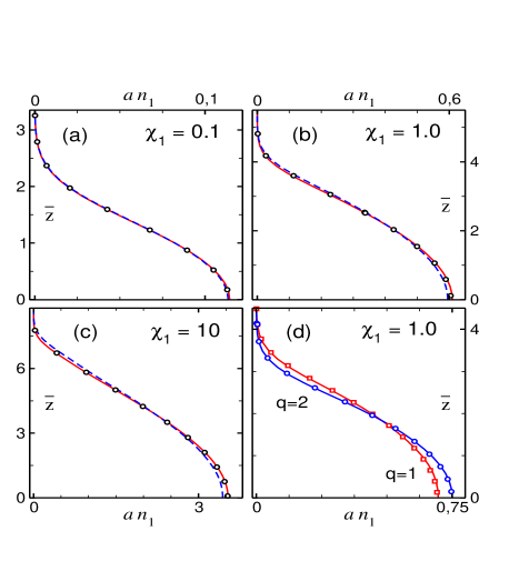
Figure 2: (Color online) Axial density profile $n_{1}(\overline{z})$ of cigar-shaped condensates in a harmonic trap with aspect ratio $\lambda=\omega_{z}/\omega_{\bot}=0.1$ and $\chi_{1}=0.1,1$ and $10$. (a)-(c): Ground-state ($q=0$) equilibrium configuration. (d): Equilibrium configuration compatible with a vortex of charge $q=1$ and $2$. Solid lines are numerical results obtained from our effective 1D equation (23). Dashed lines are numerical results obtained from the 1D NPSE by Salasnich et al. Open symbols are exact numerical results obtained from the full 3D GPE.

Figure 2 shows the axial density profile $n_{1}(\overline{z})$ of cigar-shaped condensates in a harmonic trap with aspect ratio $\lambda=\omega_{z}/\omega_{\bot}=0.1$ in the different relevant regimes, which, for a given vorticity $q$, are completely characterized by the value of the sole parameter $\chi_{1}$. Figures 2(a)–2(c) correspond to the ground-state ($q=0$) equilibrium configuration, while Fig. 2(d) shows the equilibrium configuration compatible with a vortex of charge $q=1$ and $2$. Solid lines are numerical results obtained from our effective 1D equation (23). Dashed lines are numerical results obtained from the 1D NPSE by Salasnich et al. and open symbols are exact numerical results obtained from the full 3D GPE. As is apparent from Fig. 2(a), in the perturbative regime ($\chi_{1}=0.1$), both approaches are practically indistinguishable, a consequence of the fact that both have the correct perturbative limit. However, as $\chi_{1}$ increases our effective 1D equation is always more accurate [Figs. 2(b) and 2(c)], which is a consequence of the fact that our approach, unlike that by Salasnich et al., also reproduces correctly the TF limit. The difference, though small, can be clearly appreciated even for $\chi_{1}=1$. Moreover, our approach also allows treating the case of condensates containing an axisymmetric vortex, with no additional cost. Figure 2(d) shows the equilibrium configuration of condensates with a vortex of charge $q=1$ and $2$, obtained from the same effective 1D equation (23) by simply taking $\beta_{q}=2$ and $8/3$, respectively. As is apparent, the agreement with the exact numerical results (open symbols) is again very good.

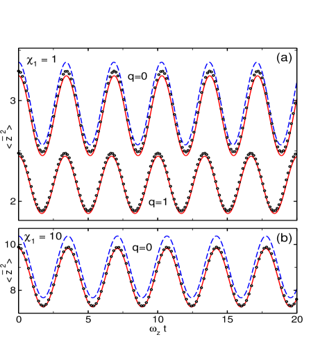
Figure 3: (Color online) Time evolution of the mean squared amplitude $\langle\overline{z}^{2}\rangle$ of cigar-shaped condensates with $\chi_{1}=1$ and $10$ and vortex charges $q=0$ and $1$ after a perturbation $\omega_{z}\rightarrow 1.1\omega_{z}$. The aspect ratio of the harmonic trap before perturbation is $\lambda=\omega_{z}/\omega_{\bot}=0.1$. Solid lines are numerical results obtained from our effective 1D equation (23). Dashed lines are numerical results obtained from the 1D NPSE by Salasnich et al. Open symbols are exact numerical results obtained from the full 3D GPE.

Our approach also reproduces very accurately the time evolution of cigar-shaped condensates. To see this we start from the equilibrium configuration of condensates confined in a harmonic trap with aspect ratio $\lambda=\omega_{z}/\omega_{\bot}=0.1$. Then we introduce a sudden perturbation by increasing the axial confinement frequency as $\omega_{z}\rightarrow 1.1\omega_{z}$ and follow the subsequent evolution in time of the mean squared axial amplitude $\langle\overline{z}^{2}\rangle=\int d\overline{z}\,\overline{z}^{2}n_{1}(\overline{z},t)$. Figure 3 shows the corresponding results obtained for condensates with $\chi_{1}=1$ and $10$ and vortex charges $q=0$ and $1$. As before solid lines are numerical results obtained from our effective 1D equation (23), dashed lines are numerical results obtained from the 1D NPSE by Salasnich et al., and open symbols are exact numerical results obtained from the full 3D GPE. For $\chi_{1}=0.1$ (not shown in the figure) both approaches produce results that are indistinguishable on the scale of the figure from the exact results. It is apparent that our approach is more accurate than that by Salasnich et al. Moreover, as Fig. 3(a) shows, it also produces very accurate results for condensates containing an axisymmetric vortex. Note also that for $\chi_{1}=1$ and $q=0$, Fig. 3(a) shows that the results from the 1D NPSE begin to dephase at large times. To see this behavior more clearly, it is convenient to consider a more complex situation. To this end we consider a BEC with $\chi_{1}=2$ in a harmonic trap with $\lambda=0.1$, subject to a blue-detuned laser beam modelled by the Gaussian potential

$$V(z)=V_{0}\exp(-z^{2}/2z_{0}^{2}),$$ (37)

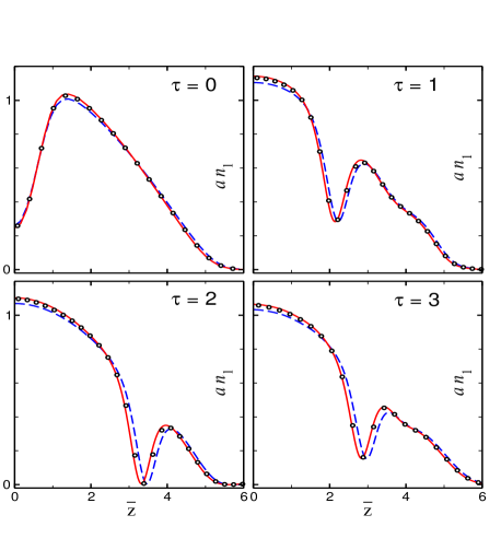
Figure 4: (Color online) Evolution of the axial density profile $n_{1}(\overline{z})$ of a cigar-shaped condensate in a harmonic trap with aspect ratio $\lambda=\omega_{z}/\omega_{\bot}=0.1$ and $\chi_{1}=2$ for different times $\tau=\omega_{z}t$. Solid lines are numerical results obtained from our effective 1D equation (23). Dashed lines are numerical results obtained from the 1D NPSE by Salasnich et al. Open symbols are exact numerical results obtained from the full 3D GPE.

with $V_{0}=12\hbar\omega_{z}$ and $z_{0}=\sqrt{2\lambda}a_{z}$. We let the condensate reach its equilibrium configuration and then, at $\tau=\omega_{z}t=0$, we suddenly switch off the laser beam and let the system evolve in the harmonic trap. Figure 4 shows the time evolution of the axial density profile $n_{1}(\overline{z})$. Solid lines are numerical results obtained from our effective 1D equation (23), dashed lines are numerical results obtained from the 1D NPSE by Salasnich et al., and open symbols are exact numerical results obtained from the full 3D GPE. At $\tau=1$ one recognizes in each half-axis a dark solitonlike structure that develops from the initial configuration and propagates toward the corresponding condensate edge (only the positive half-axis is represented in the figure). At $\tau=2$ the soliton becomes black and it comes back toward the condensate center for $\tau>2$, as can be seen in the snapshot at $\tau=3$. This figure demonstrates again that our approach is more accurate than that by Salasnich et al. In particular, it is apparent that the results obtained from the 1D NPSE become somewhat dephased with respect to the exact results.

III III. DISK-SHAPED CONDENSATES

Consider now a condensate confined in an anisotropic trap that is much stronger in the axial than in the radial direction. In this case, using similar arguments as before, one can resort to the adiabatic approximation and assume that at every instant of time the (fast) axial degrees of freedom adjust instantaneously to the equilibrium configuration compatible with the radial configuration occurring at that time. Under these circumstances the condensate wave function can be factorized as

$$\psi(\mathbf{r},t)=\varphi(\mathbf{r}_{\bot},t)\phi(z;n_{2}(\mathbf{r}_{\bot},t)),$$ (38)

where $n_{2}(\mathbf{r}_{\bot},t)$ is the local condensate density per unit area characterizing the radial configuration

$$n_{2}(\mathbf{r}_{\bot},t)\equiv N\int dz|\psi(\mathbf{r}_{\bot},z,t)|^{2}.$$ (39)

The normalization condition

$$\int dz|\phi(z;n_{2})|^{2}=1$$ (40)

leads to

$$n_{2}(\mathbf{r}_{\bot},t)=N|\varphi(\mathbf{r}_{\bot},t)|^{2}.$$ (41)

After substituting Eq. (38) into Eq. (1), one arrives at

$$\left(i\hbar\frac{\partial\varphi}{\partial t}+\frac{\hbar^{2}}{2m}\nabla_{\bot}^{2}\varphi-V_{\bot}(\mathbf{r}_{\bot})\varphi\right)\phi(z;n_{2})=\\ \left(-\frac{\hbar^{2}}{2m}\frac{\partial^{2}\phi}{\partial z^{2}}+V_{z}(z)\phi+gn_{2}(\mathbf{r}_{\bot},t)\left|\phi\right|^{2}\phi\right)\varphi(\mathbf{r}_{\bot},t),$$ (42)

where as before we have assumed the confining potential to be separable. Integrating out the fast degrees of freedom one obtains

$$i\hbar\frac{\partial\varphi}{\partial t}=-\frac{\hbar^{2}}{2m}\nabla_{\bot}^{2}\varphi+V_{\bot}(\mathbf{r}_{\bot})\varphi+\mu_{z}(n_{2})\varphi,$$ (43)

with

$$\mu_{z}(n_{2})\equiv\int dz\,\phi^{\ast}\left(-\frac{\hbar^{2}}{2m}\frac{\partial^{2}}{\partial z^{2}}+V_{z}(z)+gn_{2}\left|\phi\right|^{2}\right)\phi.$$ (44)

Substituting Eq. (43) in Eq. (42) one finds

$$\left(-\frac{\hbar^{2}}{2m}\frac{\partial^{2}}{\partial z^{2}}+V_{z}(z)+gn_{2}\left|\phi\right|^{2}\right)\phi=\mu_{z}(n_{2})\phi.$$ (45)

The effective 2D mean-field equation (43) governs the radial dynamics of disk-shaped BECs, incorporating the contribution from the axial degrees of freedom through the (axial) local chemical potential $\mu_{z}(n_{2})$. This quantity, in turn, follows from the stationary Gross-Pitaevskii equation (45) determining the axial configuration $\phi(z;n_{2})$.

The condensate stationary states

$$\varphi(\mathbf{r}_{\bot},t)=\varphi_{0}(\mathbf{r}_{\bot})e^{-i\mu t/\hbar}$$ (46)

satisfy

$$-\frac{\hbar^{2}}{2m}\nabla_{\bot}^{2}\varphi_{0}+V_{\bot}(\mathbf{r}_{\bot})\varphi_{0}+\mu_{z}(n_{2})\varphi_{0}=\mu\varphi_{0},$$ (47)

where the chemical potential$\ \mu$ guarantees the condition $\int d^{2}\mathbf{r}_{\bot}|\varphi(\mathbf{r}_{\bot},t)|^{2}=1$. When the typical length scale $\Delta_{\bot}$ of the spatial variations of $\varphi_{0}$ is much greater than the corresponding radial healing length, i.e.,

$$\Delta_{\bot}\gg\frac{\hbar}{\sqrt{2m(\mu_{z}(n_{2})-\frac{1}{2}\hbar\omega_{z})}},$$ (48)

then Eq. (47) reduces to the local density approximation

$$\mu=\mu_{z}(n_{2})+V_{\bot}(\mathbf{r}_{\bot}).$$ (49)

We shall consider in what follows disk-shaped condensates confined in the axial direction by a harmonic potential characterized by an oscillator length $a_{z}=\sqrt{\hbar/m\omega_{z}}$,

$$V(\mathbf{r})=\frac{1}{2}m\omega_{z}^{2}z^{2}+V_{\bot}(\mathbf{r}_{\bot}).$$ (50)

In terms of dimensionless variables $\overline{z}=z/a_{z}$, $\overline{\phi}=\sqrt{a_{z}}\phi$, and $\overline{\mu}_{z}=\mu_{z}/\hbar\omega_{z}$, the axial equation (45) reads

$$\left(-\frac{1}{2}\frac{\partial^{2}}{\partial\overline{z}^{2}}+\frac{1}{2}\overline{z}^{2}+4\pi aa_{z}n_{2}\left|\overline{\phi}\right|^{2}\right)\overline{\phi}=\overline{\mu}_{z}(n_{2})\overline{\phi}.$$ (51)

In Ref. Previos , we found the following expression for the axial local chemical potential $\overline{\mu}_{z}$ as a function of the condensate density per unit area $n_{2}$:

$$\overline{\mu}_{z}(n_{2})\equiv{}\!\frac{1}{8}\!\left[\!\left(\!\eta+\!\sqrt{\eta^{2}\!-\!\xi_{1}^{6}}\right)^{\frac{1}{3}}\!+\!\left(\!\eta\!-\!\sqrt{\eta^{2}\!-\!\xi_{1}^{6}}\right)^{\frac{1}{3}}\!\!-\!\xi_{1}\right]^{2},$$ (52)

where $\eta=4+6\xi_{1}-\xi_{1}^{3}+24\pi aa_{z}n_{2}$ and $\xi_{1}\equiv(\kappa_{2}-1)$ with

$$\kappa_{2}^{-1}(\overline{n}_{2}) \equiv\sqrt{2/\pi}+\Theta(\overline{n}_{2}-0.1)$$

$$\times \left(1-\sqrt{2/\pi}\right)\left(1-(10\overline{n}_{2})^{-1/5}\right).$$ (53)

In the above equation, $\Theta(x)$ is the step function and $\overline{n}_{2}\equiv aa_{z}n_{2}$ is the only relevant parameter. Note that in Ref. Previos we used the same expression (53) but in terms of the dimensionless parameter $\chi_{2}\equiv Na/\lambda^{2}a_{z}$ instead of $\overline{n}_{2}$. It was shown there that $\chi_{2}$ is the only relevant parameter for the description of harmonically trapped disk-shaped condensates, so that $\overline{n}_{2}$ and $\chi_{2}$ are directly related to each other. In particular, the quasi-2D perturbative regime corresponds to $\chi_{2}\ll 1\leftrightarrow\overline{n}_{2}\ll 1$, while in the TF regime $\chi_{2}\gg 1\leftrightarrow\overline{n}_{2}\gg 1$. On the other hand, as explained in Ref. Previos , the (slowly varying) last term in Eq. (53) was conveniently introduced to ensure that in the TF limit $\kappa_{2}^{-1}\rightarrow 1$, its specific functional form being not very relevant. This way one guarantees the correct expression for $\overline{\mu}_{z}(n_{2})$ in both the TF and the perturbative regimes. On these grounds and taking into account that $\chi_{2}\sim$ $\overline{n}_{2}$, we have simply made the substitution $\chi_{2}\rightarrow$ $\overline{n}_{2}$ in Eq. (53) which now becomes a very slowly varying function of $\overline{n}_{2}$.

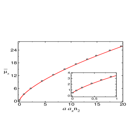
Figure 5: (Color online) Theoretical prediction for the axial local chemical potential $\overline{\mu}_{z}$ as a function of $aa_{z}n_{2}$ (solid lines). The open circles are exact numerical results obtained by solving the stationary Gross-Pitaevskii equation (51).

Figure 5 shows the theoretical prediction for $\overline{\mu}_{z}$ obtained from Eq. (52) (solid lines) along with the exact results obtained from the numerical solution of the axial equation (51) (open circles). As is apparent, not only does Eq. (52) have the correct limit in the two relevant extreme regimes, but it also accounts accurately for the corresponding dimensional crossover.

Substituting Eqs. (52) and (53) with $n_{2}=N|\varphi(\mathbf{r}_{\bot},t)|^{2}$ into Eq. (43), we finally obtain the desired effective 2D equation. This equation governs the transverse dynamics of arbitrary mean-field disk-shaped condensates with repulsive interatomic interactions, accounting properly for the effects from the axial degrees of freedom. In the quasi-2D mean-field regime ($aa_{z}n_{2}\ll 1$), it reduces to

$$i\hbar\frac{\partial\varphi}{\partial t}=-\frac{\hbar^{2}}{2m}\nabla_{\bot}^{2}\varphi+V_{\bot}(\mathbf{r}_{\bot})\varphi+g_{\mathrm{2D}}N|\varphi|^{2}\varphi,$$ (54)

where $g_{\mathrm{2D}}=g/\sqrt{2\pi}\,a_{z}=2\sqrt{2\pi}aa_{z}\hbar\omega_{z}$ and we have absorbed a constant $\hbar\omega_{z}/2$ into the definition of the generic transverse potential $V_{\bot}(\mathbf{r}_{\bot})$. Similarly, in the TF regime ($aa_{z}n_{2}\gg 1$), the effective 2D equation reduces to

$$i\hbar\frac{\partial\varphi}{\partial t} =-\frac{\hbar^{2}}{2m}\nabla_{\bot}^{2}\varphi+V_{\bot}(\mathbf{r}_{\bot})\varphi$$

$$+\hbar\omega_{z}\left[(3\pi/\sqrt{2})aa_{z}N|\varphi|^{2}\right]^{2/3}\varphi.$$ (55)

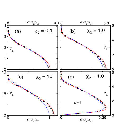
Figure 6: (Color online) Radial density profile $n_{2}(r_{\bot})$ of disk-shaped condensates in a harmonic trap with aspect ratio $\lambda=\omega_{z}/\omega_{\bot}=10$ and $\chi_{2}=0.1,1,$ and $10$. (a)-(c): Ground-state ($q=0$) equilibrium configuration. (d): Equilibrium configuration compatible with a vortex of charge $q=1$. Solid lines are numerical results obtained from our effective 2D equation (43). Dashed lines are numerical results obtained from the 2D NPSE by Salasnich et al. Open symbols are exact numerical results obtained from the full 3D GPE.

It can be easily verified that both Eq. (54) and Eq. (55) are the correct limits of the underlying 3D GPE. As in the 1D case, our effective 2D equation permits one to derive analytical expressions for ground-state properties of disk-shaped condensates such as the chemical potential, condensate radius, radial density profile, and local sound velocity. These analytical expressions reduce to the correct formulas in both the TF and the perturbative regimes, and remain valid and accurate in between these two limiting cases. Since the calculations are more complicated than before we refer the reader to our previous work for details Previos .

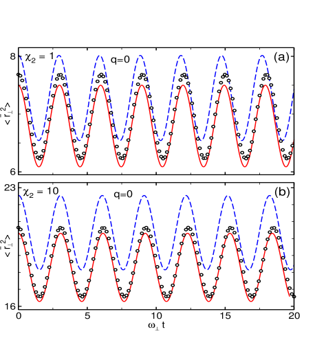
Figure 7: (Color online) Time evolution of the mean squared amplitude $\langle\overline{r}_{\bot}^{2}\rangle$ of disk-shaped condensates with $\chi_{2}=1$ and $10$ after a perturbation $\omega_{\bot}\rightarrow 1.1\omega_{\bot}$. The aspect ratio of the harmonic trap before perturbation is $\lambda=\omega_{z}/\omega_{\bot}=10$. Solid lines are numerical results obtained from our effective 2D equation (43). Dashed lines are numerical results obtained from the 2D NPSE by Salasnich et al. Open symbols are exact numerical results obtained from the full 3D GPE.

Next we shall consider disk-shaped condensates in a confining potential that is also harmonic in the radial direction $V_{\bot}(r_{\bot})=\frac{1}{2}m\omega_{\bot}^{2}r_{\bot}^{2}$. The corresponding oscillator length is $a_{\bot}=\sqrt{\hbar/m\omega_{\bot}}$ and the trap aspect ratio now satisfies the inequality $\lambda=\omega_{z}/\omega_{\bot}\gg 1$. In Fig. 6 we show the radial density profile $n_{2}(r_{\bot})$ of condensates in a trap with $\lambda=10$, in the different relevant regimes characterized by the parameter $\chi_{2}$. The dimensionless variable $\overline{r}_{\bot}$ is defined as $\overline{r}_{\bot}=r_{\bot}/$ $a_{\bot}$. Figures 6(a)–6(c) correspond to the ground-state ($q=0$) equilibrium configuration, while Fig. 6(d) corresponds to the equilibrium configuration compatible with a $q=1$ vortex. Solid lines are numerical results obtained from our effective 2D equation (43) with $\mu_{z}(|\varphi|^{2})$ given by Eqs. (52) and (53). Dashed lines are numerical results obtained from the 2D NPSE by Salasnich et al. Reatto1 and open symbols are exact numerical results obtained from the full 3D GPE. In the perturbative regime, for $\chi_{2}=0.1$, the 2D NPSE is somewhat more accurate. This is precisely the parameter region where the error of our effective equation is maximum. As $\chi_{2}$ increases, our equation becomes more accurate. This can be appreciated in Figs. 6(b)–6(d) which show that our results remain very accurate as $\chi_{2}$ increases. On the contrary, the error of the 2D NPSE increases with $\chi_{2}$, being of the order of $5\%$ for $\chi_{2}=1$ and of the order of $10\%$ for $\chi_{2}=10$. This is a consequence of the fact that the underlying (Gaussian) variational wave function that leads to the 2D NPSE cannot reproduce properly the TF regime.

To investigate the validity of our effective equation in time-dependent problems we have followed the same procedure as before. We start from the equilibrium configuration of condensates confined in a harmonic trap with $\lambda=10$. We then perturb the system by changing instantaneously the radial confinement frequency as $\omega_{\bot}\rightarrow 1.1\omega_{\bot}$ and follow the subsequent evolution in time of the mean squared radial amplitude $\langle\overline{r}_{\bot}^{2}\rangle=\int d^{2}\overline{\mathbf{r}}_{\bot}\,\overline{r}_{\bot}^{2}n_{2}(\overline{r}_{\bot},t)$. Figure 7 shows the corresponding results for condensates with $\chi_{2}=1$ and $10$. Solid lines are numerical results obtained from our effective 2D equation (43) with $\mu_{z}(|\varphi|^{2})$ given by Eqs. (52) and (53), dashed lines are numerical results obtained from the 2D NPSE, and open symbols are exact numerical results obtained from the full 3D GPE. As is apparent from the figure, our effective 2D equation is again more accurate than the 2D NPSE by Salasnich et al.

IV IV. CONCLUSION

In this work, by applying the standard adiabatic approximation and using the analytical expression for the transverse local chemical potential obtained in our previous work Previos , we have derived an effective 1D equation that governs the axial dynamics of mean-field cigar-shaped condensates with repulsive interatomic interactions. This equation, which incorporates accurately the contribution from the transverse degrees of freedom, has the correct limits in both the quasi-1D mean-field regime and the TF regime. Since our expression for the local chemical potential is very accurate, the validity of the above equation relies almost exclusively on the validity of the well established adiabatic approximation.

We have compared our effective 1D equation with the 1D NPSE by Salasnich et al. which provides more accurate results than any other previously proposed effective equation. We have demonstrated that our effective 1D equation is more accurate, which, in part, is a consequence of the fact that our approach, unlike that by Salasnich et al., reproduces correctly the TF limit. Moreover, our equation allows treating condensates containing an axisymmetric vortex with no additional cost. Because of its simplicity, it also permits one to derive fully analytical expressions for ground-state properties such as the chemical potential, axial length, axial density profile, and local sound velocity. These analytical expressions reduce to the correct analytical formulas in both the TF and the perturbative regimes, and remain valid and accurate in between these two limiting cases.

Following the same procedure we have also derived an effective 2D equation that governs the transverse dynamics of mean-field disk-shaped condensates, accounting properly for the contribution from the axial degrees of freedom. This equation is also more accurate than the 2D NPSE by Salasnich et al. As in the 1D case, from this effective equation, which also has the correct limits in both the quasi-2D and the TF regime, one can derive analytical expressions for ground-state properties of cigar-shaped condensates such as the chemical potential, condensate radius, radial density profile, and local sound velocity.

- (1) M. H. Anderson, J. R. Ensher, M. R. Matthews, C. E. Wieman, and E. A. Cornell, Science 269, 198 (1995).
- (2) K. B. Davis, M. -O. Mewes, M. R. Andrews, N. J. van Druten, D. S. Durfee, D. M. Kurn, and W. Ketterle, Phys. Rev. Lett. 75, 3969 (1995).
- (3) C. C. Bradley, C. A. Sackett, and R. G. Hulet, Phys. Rev. Lett. 78, 985 (1997).
- (4) E. P. Gross, Nuovo Cimento 20, 454 (1961); J. Math. Phys. 4, 195 (1963); L. P. Pitaevskii, Zh. Eksp. Teor. Fiz. 40, 646 (1961) [Sov. Phys. JETP 13, 451 (1961)].
- (5) A. Muñoz Mateo and V. Delgado, Phys. Rev. Lett. 97, 180409 (2006).
- (6) M. Olshanii, Phys. Rev. Lett. 81, 938 (1998).
- (7) D. S. Petrov, G. V. Shlyapnikov, and J. T. M. Walraven, Phys. Rev. Lett. 85, 3745 (2000).
- (8) D. S. Petrov, M. Holzmann, and G. V. Shlyapnikov, Phys. Rev. Lett. 84, 2551 (2000).
- (9) V. Dunjko, V. Lorent, and M. Olshanii, Phys. Rev. Lett. 86, 5413 (2001).
- (10) K. K. Das, Phys. Rev. A 66, 053612 (2002).
- (11) A. Görlitz, J. M. Vogels, A. E. Leanhardt, C. Raman, T. L. Gustavson, J. R. Abo-Shaeer, A. P. Chikkatur, S. Gupta, S. Inouye, T. Rosenband, and W. Ketterle, Phys. Rev. Lett. 87, 130402 (2001).
- (12) C. Menotti and S. Stringari, Phys. Rev. A 66, 043610 (2002).
- (13) A. D. Jackson, G. M. Kavoulakis, and C. J. Pethick, Phys. Rev. A 58, 2417 (1998).
- (14) M. L. Chiofalo and M. P. Tosi, Phys. Lett. A 268, 406 (2000).
- (15) L. Salasnich, A. Parola, and L. Reatto, Phys. Rev. A 65, 043614 (2002).
- (16) P. Massignan and M. Modugno, Phys. Rev. A 67, 023614 (2003).
- (17) A. M. Kamchatnov and V. S. Shchesnovich, Phys. Rev. A 70, 023604 (2004).
- (18) W. Zhang and L. You, Phys. Rev. A 71, 025603 (2005).
- (19) M. Krämer, C. Menotti and M. Modugno, J. Low Temp. Phys. 138, 729 (2005).
- (20) A. Muñoz Mateo and V. Delgado, Phys. Rev. A 75, 063610 (2007); Phys. Rev. A 74, 065602 (2006).
- (21) J. A. Huhtamäki, M. Möttönen, T. Isoshima, V. Pietilä, and S. M. Virtanen, Phys. Rev. Lett. 97, 110406 (2006).
- (22) V. M. Pérez-García, H. Michinel, J. I. Cirac, M. Lewenstein, and P. Zoller, Phys. Rev. A 56, 1424 (1997); Phys. Rev. Lett. 77, 5320 (1996).
- (23) L. Salasnich, A. Parola, and L. Reatto, Phys. Rev. A 69, 045601 (2004).