Investigation of A Lattice Boltzmann Model with a Variable Speed of Sound

Abstract

A Lattice Boltzmann model is considered in which the speed of sound can be varied independently of the other parameters. The range over which the speed of sound can be varied is investigated and good agreement is found between simulations and theory. The onset of non-linear effects due to variations in the speed of sound is also investigated and good agreement is again found with theory. It is also shown that the fluid viscosity is not altered by changing the speed of sound.

1 Introduction

The lattice Boltzmann model (LBM) is a numerical technique for fluid simulation which has become increasingly popular in recent years [1, 2, 3, 4]. The LBM originates from the lattice gas model (LGM) [5, 6, 7, 8] were fluid particles are constrained to move on a regular lattice such that their collisions conserve mass and momentum. The particles are further constrained to move with unit velocity and with a maximum occupancy of one particle per grid direction per grid site. The evolution of the LBM from the lattice gas model involved a number of key developments. The Boolean particle number (1 if a particle is present and 0 otherwise) was replaced by a real number, later recognized as the distribution function, representing an ensemble average of the particle occupation [9]; this removed the noise associated with the relatively small number of fluid particles represented in the LGM. Obtaining an ensemble average of the particle collisions is not straightforward but the process was simplified to depend only on the link direction [10] and the isotropy of the model [11]. Finally the particle-particle collisions were replaced by considering the distribution functions relaxing toward a Maxwell-Boltzmann equilibrium distribution [12].

The LBM is referred to as an incompressible technique because the LBM scheme can be shown to satisfy the incompressible Navier-Stokes equation in the limit that the density, $\rho$, does not vary in space or time. However, when applying the LBM, there is no restriction on the density to remain constant and in many applications the density will vary in space and/or time. In practice the ‘incompressible’ nature of the LBM is interpreted as requiring that any density variations are small or that the density varies only slowly in space and time. In this limit it is possible to simulate phenomena such as acoustic waves where a density variation is required, provided the variation is small [13, 14, 15].

In the LBM, pressure is defined through the equation of state, see for example [2], $p=c^{2}\rho$, where $c$ is the speed of sound which takes a fixed value in any simulation, dependent only on external factors such as the shape of the simulation grid. Thus we see that the speed of sound controls the relationship between the density and the pressure and therefore the compressibility of the fluid. To model fluids with different compressibility we require to be able to change the speed of sound in the simulation. Here we consider a model with a variable speed of sound and investigate the non-linear aspects of sound wave propagation.

2 The lattice Boltzmann model

In this section we briefly consider the standard LBM on a square grid in two dimensions. In the LBM the distribution functions, $f_{i}(\mbox{\boldmath{$x$}},t)$, for $i$= 0-8 evolve on a regular grid according to the Boltzmann equation [16], as

$$f_{i}(\mbox{\boldmath{$x$}}+\mbox{\boldmath{$e$}}_{i},t+1)-f_{i}(\mbox{\boldmath{$x$}},t)=-\frac{1}{\tau}(f_{i}-\overline{f}_{i}),$$ (1)

where $\mbox{\boldmath{$e$}}_{i}$ = $(\cos[\pi(i-1)/2],\sin[\pi(i-1)/2])$ for $i$ = 1-4, and $\mbox{\boldmath{$e$}}_{i}$ = $\sqrt{2}(\cos[\pi(i-9/2)/2],\sin[\pi(i-9/2)/2])$ for $i$ = 5-8 are link vectors on the grid and $\mbox{\boldmath{$e$}}_{0}$ = (0,0). The left hand side of equation (1) represents streaming of the distribution function from one site to a neighbouring site. The right hand side is the Bhatnagar, Gross and Krook (BGK) collision operator [17, 12, 18]. The equilibrium distribution function $\overline{f}_{i}$ is given by [16]

$$\overline{f}_{i}=w_{i}\rho\left[1+3\mbox{\boldmath{$e$}}_{i}\cdot\mbox{\boldmath{$u$}}+\frac{9}{2}(\mbox{\boldmath{$e$}}_{i}\cdot\mbox{\boldmath{$u$}})^{2}-\frac{3}{2}u^{2}\right],$$ (2)

where the fluid density, $\rho$, and velocity, $u$ are found from the distribution function as

$$\rho=\sum_{i=0}^{8}f_{i}\quad\mbox{and}\quad\rho\mbox{\boldmath{$u$}}=\sum_{i=0}^{8}f_{i}\mbox{\boldmath{$e$}}_{i}$$ (3)

and where $w_{0}=4/9$, $w_{i}$ = 1/9 for $i$=1-4, and $w_{i}$ = 1/36 for $i$ = 5-8. The relaxation time, $\tau$, determines the rate at which the distribution functions relax to their equilibrium values; it determines the fluid viscosity, $\nu$, as

$$\nu=\frac{(2\tau-1)}{6}.$$ (4)

Equation (1) can be modified by the addition of an extra source term. This approach has been used to implement a body force [19] and also to simulate non-ideal equations of state such as phase separation [20].

3 A lattice Boltzmann Model with a Variable Speed of Sound

One method for achieving a variable speed of sound was proposed by Alexander et al. [21] who considered a model on a hexagonal grid with an altered equilibrium distribution function in which the ratio of ‘rest particles’ ($f_{0}$) to ‘moving particles’ ($f_{i},i\neq 0$) can be altered. Simulations performed using this model [21] showed that the speed of sound can be varied between 0 and approximately 0.65 with good agreement between theory and simulation for speed less than approximately 0.4. Above 0.4 there is some deviation between theory and simulation. In this model the viscosity was also found to be a function of the variable speed of sound.

An alternative approach was proposed by Yu and Zhao [22]. They introduced an attractive force which produced a variable speed of sound which was dependent on the amplitude of the introduced force. The model was verified by measuring the Doppler shift and the Mach cone for Mach numbers less than and greater then unity respectively.

Here we consider the following LBM:

$$f_{i}(\mbox{\boldmath{$x$}}+\mbox{\boldmath{$e$}}_{i},t+1)-f_{i}(\mbox{\boldmath{$x$}},t)=-\frac{1}{\tau}(f_{i}-\overline{f}_{i})+3w_{i}\alpha\mbox{\boldmath{$\nabla$}}\rho\cdot\mbox{\boldmath{$e$}}_{i},$$ (5)

where $\overline{f}_{i}$ and $w_{i}$ are defined as previously and the additional term on the right-hand side of equation (5) represents a body force $\alpha\nabla\rho$, see for example [19]. This is effectively the same as the model of Yu and Zhao [22], except that the forcing term is expressed explicitly as proportional to the density gradient and the amplitude term, $\alpha$ is not restricted to be positive. Performing a Chapman-Enskog expansion [8] we can write the Navier-Stokes equation in the form

$$\partial_{t}u_{\alpha}+u_{\beta}\partial_{\beta}u_{\alpha}=-\frac{1}{\rho}\partial_{\alpha}\left(c_{1}^{2}-\alpha\right)\rho+\nu\partial_{\beta}(\partial_{\alpha}u_{\beta}+\partial_{\beta}u_{\alpha}),$$ (6)

where

$$\nu=\frac{2\tau-1}{6}$$ (7)

as before, and we have assumed that the derivatives of $\rho$ can be neglected except where they appear in the pressure term. This is the Navier-Stokes equation for a fluid which has pressure $p=c_{e}^{2}\rho$, where $c_{e}$ is the effective speed of sound which is given by

$$c_{e}=\sqrt{\left(c_{1}^{2}-\alpha\right)}.$$ (8)

Thus by introducing an additional term to the Boltzmann equation which acts as a body force proportional to the density gradient, we have included a force which increases or decreases (depending on the sign of $\alpha$) the pressure forcing term in the Navier-Stokes equation, and hence the speed of sound in the model.

A number of models, based on the cellular automata (CA) approach of the LGM, have also been applied to simulate acoustic waves as well as Burgers’ equation. Mora [23] introduced the phononic lattice solid model which obeyed a Boltzmann equation and satisfied the acoustic wave equation in the macroscopic limit. The Boltzmann equation was solved using a finite-difference scheme. This model was further developed [24] in the phononic lattice solid by interpolation model in which the particle number densities move along the lattice links in the same manner as the distribution functions in the LGM and LBM. Unlike the lattice gas particles they travel at different speeds and so, in general, do not arrive at a grid site after each time step. The number densities are therefore interpolated to find the value at each site.

CA models for Burgers’ equation have also been considered. The model of Boghosian and Levermore [25] was based on the LGM approach and was shown to follow the solution of Burgers’ equation. The convergence of the model was also established [26]. Following the development of the LBM from the LGM [9, 10, 11], Elton [27] considered a CA model for Burgers’ equation based on the mean occupation number rather than discrete particles. The model compared favourably with a finite difference solution of Burgers’ equation. A quantum lattice gas model [28] and an intrinsically stable entropic model [29] have also been proposed recently. Each of these models provides a simulation method which satisfies Burgers’ equation. This is different to the model investigated here which satisfies the Navier-Stokes equation and is also capable of simulating non-linear acoustic waves whose behaviour, for the case $\alpha=0$, has been shown to be in good agreement with Burgers’ equation [14]. This means that it is capable of simulating the interaction between acoustic waves and fluid flow, see for example [15, 30, 31, 32].

4 Numerical Simulations

The variation in the speed of sound was investigated in the following simulations of plane acoustic wave propagating in an unbound media. This if effectively a one dimensional problem so a gird was used with only 4 points in the $y$-direction. The grid had $L$ points in the $x$-direction and was initialised with zero velocity and unit density. Periodic boundary conditions were applied at $y$ = 0 and $y$ = 4. At $x$ = 0 a boundary condition was applied in which the density was varied in a sinusoidal manner with a period of 500 time-steps, the velocity at this grid boundary was maintained at zero. At $y$ = $L$ a boundary condition of $\rho$ = 1 and $u$ = 0 was applied. $L$ was selected to be large enough so that the density disturbance does not reach $x$ = $L$ during the measurement window. From these simulations the speed of sound was found in two ways: 1) from the time taken for the wave to pass between two points at a known separation; and 2) since we are dealing with a low amplitude plane harmonic wave, $c_{e}$ can be derived from [33] $u(\mbox{\boldmath{$x$}}^{*},t^{*})/c_{e}=[\rho(\mbox{\boldmath{$x$}}^{*},t^{*})-\rho_{0}]/\rho_{0}$, where $u(\mbox{\boldmath{$x$}}^{*},t^{*})$ and $\rho(\mbox{\boldmath{$x$}}^{*},t^{*})$ are the fluid velocity and density respectively, at some position $\mbox{\boldmath{$x$}}^{*}$ and time $t^{*}$; here we selected $\mbox{\boldmath{$x$}}^{*}$ and $t^{*}$ such that they correspond to a pressure and velocity maximum. The results are shown in figure 1 where there is excellent agreement between the measured values of $c_{e}$ and the theoretical values given by equation (8) over a range of $\alpha$. At $\alpha=1/3$ we have $c_{e}=0$ giving an upper limit for $\alpha$. Now $\alpha=-2/3$ gives $c_{e}=1$ which would appear to be an upper limit since this is the speed with which the distribution functions propagate and so is the maximum speed information about the density, pressure and velocity can be transmitted through the fluid. Initial simulations were performed using a simple forward difference scheme to calculate the pressure gradient. In this case the model became unstable as $c_{e}$ approached unit, as would be expected. When a central difference technique was applied to calculate the density gradient the model was found to remain stable as $c_{e}$ approaches unity. Indeed it was found to remain stable for higher values of $c_{e}$ ($\alpha<$ -2/3) and the simulated density waves were observed to propagate with $c_{e}>$ 1. The transfer of information at a speed greater than unity can be understood with the introduction of a central difference scheme to calculate the ‘pressure’ forcing term. Consider a density distribution where $\rho(x)=\rho_{0}$ everywhere at t=0, except for $\rho(x_{0})=\rho_{0}+\delta\rho$. Then at $x=x_{0}+1$ the density gradient (calculated using a central difference scheme) will be non-zero. In the case of $\alpha<$ 0 this will give a forcing term that will cause the value of the distribution function travelling in the positive direction at $x_{0}+1$ to increase. This information (about a density increase at $x_{0}$) will then be passed on to $x_{0}$+2 at t=1 by the streaming action. As seen in figure 1 this is a limited effect; however, it suggests that LB schemes in which the speed of sound is significantly greater than unit may be possible if a longer range action is applied. The largest value of $c_{e}$ which was observed to remain stable was $c_{e}$ = 1.125. The validity of simulations with $c_{e}>$ 1 has not been established and requires further investigation. The remainder of the simulations presented here have have $c_{e}<$ 1.

To further investigate the effectiveness of the model two progressive sound waves with $\lambda=4000$ were initialised with the same velocity amplitude: $u(x,t=0)=u_{0}\sin(kx)$, $v(x,t=0)=0$ and density profile $\rho^{(i)}(x,t=0)=\rho_{0}^{(i)}(1+u^{0}/c_{e}^{(i)})\sin(kx)$, for $i$ = 1, 2; where $c_{e}^{(i)}$ is found from $\alpha^{(i)}$ with $\alpha^{(1)}$ = 0.2933 and $\alpha^{(2)}$ = -0.47667. This gives $c_{e}^{(1)}$ = 0.2 and $c_{e}^{(2)}$ = 0.9 such that $c_{e}^{(2)}/c_{e}^{(1)}=4.5$. The ambient density $\rho_{0}^{(i)}$ is also free to be varied, however, in the simulations we used $\rho_{0}^{(1)}=\rho_{0}^{(2)}=1$ and $u_{0}=0.002$. For these two waves we can calculate the shock development distance given by

$$\sigma^{(i)}=\frac{1}{\epsilon M^{(i)}k},$$ (9)

where $M^{(i)}=u/c_{e}^{(i)}$ is the Mach number, $k=2\pi/\lambda$ is the wavenumber and $\epsilon=1$. This is the distance over which an initially sinusoidal wave in an inviscid fluid will develop into a discontinuous wave with a sawtooth shape. Here we have $\sigma^{(1)}\simeq 16\lambda$ and $\sigma^{(2)}\simeq 72\lambda$ so we expect wave (1) (in the fluid with the lower speed of sound) to exhibit stronger non linear effects than wave (2).

Following [14] periodic boundary conditions were applied on all grid boundaries and the waves were allowed to propagate. Figure 2 shows the normalised velocities $u^{\prime}=u/u_{0}$; plotted as a function of $\phi=\omega(t-x/c_{e})$ after the waves has propagated distances of $5\lambda$, $10\lambda$ and $15\lambda$. Here $\omega$ is the angular frequency of the acoustic wave. It can clearly be seen that wave (1) exhibits strong non-linear behaviour over the first twenty wavelengths. Also shown in figure 2 is the numerical solution of Burgers’ equation [14] which describes the wave form in a viscous fluid in terms of a truncated sum of $N$ harmonics. Good agreement is observed for $x=5,10$ and 15 $\lambda$. For $x=20\lambda$ a suitable value of $N$ could not be found to give a smooth profile. Even at large $N$ oscillations were observed on the wave form around $\phi=0$ and $\phi=\pm 1$. For this reason the solution of Burgers’ equation is only shown away from these points for $x=20$ where there is again good agreement with the Boltzmann simulations. The LBM simulation of wave (2) at $x=45\lambda(=10(c_{e}^{(2)}/c_{e}^{(1)})\lambda)$ is also shown in figure 2 for comparison. The wave form is similar to that for wave (1) at $x=10\lambda$ as would be expected from equation (9) since both waves were run with a relatively low viscosity ($\nu=0.01$). A comparison with wave (1) is given in figure 3 which shows the amplitudes, $a_{n}$, of the fundamental ($n=1$) and higher ($n>1$) harmonics. The results in figure 3 were obtained by performing a fast Fourier transform on the velocity between $x=14\lambda$ and $x>20\lambda$ where the smallest number of point which were an exact multiple of 2 were used.

Figure 4 shows the long term behaviour of wave (2) for three different fluid viscosities given by $\nu$ = 1/30, 1/2 and 7/6 , the value of $\lambda$ was 400. Relatively large values of $\tau$ were selected to ensure that the wave was damped rapidly. The results are in good agreement with the exponential decay rate predicted by linear theory, see [34, 33, 13], which is also shown.

The long term behaviour of wave (2) was also considered in fluids with a lower viscosity. The decay rate per unit time is independent of the speed of sound and depends only on the wavelength of the wave and the viscosity of the fluid. This is shown in figure 5 which depicts wave (2) for a range of $\alpha$ values after around 100 periods for the wave with $\alpha=-0.65$. It is clear from figure 5 that the damping rate is the same for each value of $\alpha$; including $\alpha$ = 0 which corresponds to the standard LBM with no additional body force. The viscosity of the fluid was obtained from the simulations as

$$\nu=-\frac{1}{k^{2}t}\ln\left(\frac{u_{t=100T}}{u_{t=0}}\right)$$ (10)

and is shown in figure 6 for $\alpha=-0.6$ for values of $\tau$ between 0.501 and 0.9. Figure 6 shows good agreement between the measure viscosity and the theoretical value at large viscosities. At lower viscosities their is some deviation. For $\alpha$ = -0.6 the largest difference observed between the simulated wave amplitude after 100 periods and the theoretical value was less then 4 %. It is well known that the LBM becomes unstable as $\tau\rightarrow$ 0.5 with noise being introduced into the simulation which eventually becomes unstable. This has been observed elsewhere, for example [35] where a filter was introduced to reduce the noise. Here a filter was not required and the introduction of the body force term was not observed to significant alter the onset of instabilities. The good agreement between the simulations and the theory indicates that the introduction of a variable speed of sound using the method proposed here does not effect the viscosity of the fluid, as predicted by equations (6) and (7).

5 Conclusions

A new lattice Boltzmann model has been devised in which the speed of sound can be varied. This has been demonstrated in a number of simulations in which the speed at which a disturbance propagates in a fluid was found to agree with the theoretical speed of sound. Further, it has also been shown that the non-linearity of a pressure wave depends not only on its amplitude but also on the speed of sound in the medium through which it is propagating, as would be expected, and good agreement was found with the numerical solution of Burgers’ equation. Compared to a previous model [21], the present model has a larger range over which the speed of sound can be varied and shows better agreement with theory over the full range. Additionally the method by which the variable speed of sound is introduced does not change the viscosity of the fluid. The speed of sound is varied in the new model by a free parameter, $\alpha$, which was kept constant in space and time during the simulations presented here. This is not, however, a fundamental requirement and it is envisaged that this model could be applied such that the speed of sound varies within the simulation. For example, in a simulation of a liquid-gas or a binary fluid mixture, the speed of sound could be varied as a function of the fluid species. This could be done in much the same was as a species dependent relaxation time has been used to simulate binary fluids with different viscosities, see for example [36]. Alternatively, in a single phase fluid simulation, the speed of sound could be varied in a pre-determined manner to account for an external influence; for example a temperature gradient or an acoustical lens. The model can also be applied to simulate fluids with different compressabilities which extends the range of application of the LBM.

Figure 1: The effective speed of sound, $c_{e}$ as a function of the forcing magnitude $\alpha$.

Figure 2: The nonlinear development of the sound wave for $c_{e}$ = 0.2 over the first twenty wavelengths. Also shown for comparison is the numerical solution of Burgers’ equation (+) and the LBM simulation of a sound wave with $c_{e}=0.9$ at $x=45\lambda$ (diamonds).

Figure 3: Amplitude of the spectral components for wave (1) and wave (2) calculated over just over six wavelengths starting at $x=14\lambda$.

Figure 4: The propagation of wave(2) for three selected values of $\tau$. Also shown is the exponential decay rate predicted by linear theory.

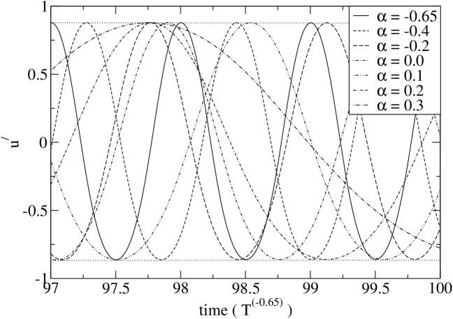
Figure 5: Propagation of wave(2) for $\tau$ = 0.52 and selected values of $\alpha$ for $97T^{(-0.65)}\leq t\leq 100T^{(-0.65)}$, where $T^{(-0.65)}$ is the period of the wave when $\alpha=-0.65$.

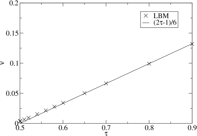
Figure 6: The fluid viscosity calculated from the decay of a wave after 100 periods with $\alpha$ = -0.6, as a function of the relaxation parameter. The solid line represents the theoretical expression.

References

- [1] S. Succi R. Benzi and M. Vergassola. The lattice Boltzmann equation: theory and applications. Physics Reports, 222:145–197, 1992.
- [2] S. Chen and G. D. Doolen. Lattice Boltzmann method for fluid flows. Annual Review of Fluid Mechanics, 30:329–364, 1998.
- [3] S. Succi. The Lattice Boltzmann Equation for Fluid Dynamics and Beyond. Oxford University Press, 2001.
- [4] D. Wolf-Gladrow. Lattice-gas cellular automata and lattice Boltzmann models. In Lecture Notes in Mathematics, volume 1725. Springer-Verlag, Heidelberg, 2000.
- [5] J. Hardy, Y. Pomeau, and O. de Pazzis. Time evolution of two-dimensional model system I: invariant states and time correlation functions. Journal of Mathematical Physics, 14:1746–1759, 1973.
- [6] J. Hardy, O. de Pazzis, and Y. Pomeau. Molecular dynamics of a classical lattice gas: Transport properties and time correlation functions. Physics Review A, 13:1949–1961, 1976.
- [7] U. Frisch, B. Hasslacher, and Y. Pomeau. Lattice-gas automata for the Navier-Stokes equation. Physical Review Letters, 56:1505–1508, 1986.
- [8] U. Frisch, D. d’ Humières, B. Hasslacher, P. Lallemand, Y. Pomeau, and J.-P. Rivet. Lattice gas hydrodynamics in two and three dimensions. Complex Systems, 1:649–707, 1987.
- [9] G. R. McNamara and G. Zanetti. Use of the Boltzmann equation to simulate lattice-gas automata. Physical Review Letters, 61:2332–2335, 1988.
- [10] F. J. Higuera and J. Jiménez. Boltzmann approach to lattice gas simulations. Europhysics Letters, 9 (7):663–668, 1989.
- [11] F. J. Higuera, S. Succi, and R. Benzi. Lattice gas dynamics with enhanced collisions. Europhysics Letters, 9 (4):345–349, 1989.
- [12] S. Chen, H. Chen, D. Martinez, and W. Matthaeus. Lattice Boltzmann model for simulation of magnetohydrodynamics. Physical Review Letters, 67 (27):3776–3779, 1991.
- [13] J. M. Buick, C. A. Greated, and D. M. Campbell. Lattice BGK simulation of sound waves. Europhysics Letters, 43:235–240, 1998.
- [14] J. M. Buick, C. L. Buckley, C. A. Greated, and J. Gilbert. Lattice Boltzmann BGK simulation of non-linear sound waves: The development of a shock front. Journal of Physics A: Mathematical and General, 33:3917–3928, 2000.
- [15] D. Haydock and J. M. Yeomans. Lattice Boltzmann simulations of acoustic streaming. Journal of Physics A: Mathematical and General, 34:5201–5213, 2001.
- [16] Y. H. Qian, D. d’ Humières, and P Lallemand. Lattice BGK models for Navier-Stokes equation. Europhysics Letters, 17 (6):479–484, 1992.
- [17] P. L. Bhatnagar, E. P. Gross, and M Krook. A model for collision processes in gases. I. Small amplitude processes in charged and neutral one-component systems. Physical Review, 94 (3):511–525, 1954.
- [18] S. Chen, Z. Wang, X. Shan, and G. D. Doolen. Lattice Boltzmann computational fluid dynamics in three dimensions. Journal of Statistical Physics, 68 (3/4):379–400, 1992.
- [19] J. M. Buick and C. A. Greated. Gravity in a lattice Boltzmann model. Physical Review E, 61:5307–5320, 2000.
- [20] X. Shan and H. Chen. Lattice Boltzmann model for simulating flows with multiple phases and components. Physical Review E, 47:1815–1819, 1993.
- [21] F. J. Alexander, H. Chen, S. Chen, and G. D. Doolen. Lattice Boltzmann model for compressible fluids. Physical Review A, 46:1967–1970, 1992.
- [22] H. You and K. Zhao. Lattice Boltzmann method for compressible flows with high Mach numbers. Physical Review E, 61:3867–3870, 2000.
- [23] P. Mora. The lattice Boltzmann phononic lattice solid. Journal of Statistical Physics, 68:591–609, 1992.
- [24] L.-J. Huang and P. Mora. The phononic lattice solid by interpolation for modelling P waves in heterogeneous media. Geophysical Journal International, 119:766–778, 1994.
- [25] B. M. Boghosian and C. D. Levermore. Cellular automaton for Burgers’ equation. Complex Systems, 1:17–29, 1987.
- [26] J. L. Lebowitz, E. Orlandi, and E. Presutti. Convergence of stochastic cellular automaton to Burgers’ equation: Fluctuations and stability. Physica D, 33:165–188, 1988.
- [27] B. H. Elton. Comparisons of lattice Boltzmann and finite difference methods for a two-dimensional viscous Burgers’s equation. SIAM Journal on Scientific Computing, 17:783–813, 1996.
- [28] J. Yepez. Quantum lattice-gas model for the Burgers equation. Journal of Statistical Physics, 107:203–224, 2002.
- [29] B. M. Boghosian, P. Love, and J. Yepez. Entropic lattice Boltzmann model for Burgers’s equation. Philosophical Transactions of the Royal Society of London A, 362:1691–1701, 2004.
- [30] D. Haydock and J. M. Yeomans. Lattice Boltzmann simulations of attenuation-driven acoustic streaming. Journal of Physics A: Mathematical and General, 36:5683–5694, 2003.
- [31] J. A. Cosgrove, J. M. Buick, D. M. Campbell, and C. A. Greated. Numerical simulation of particle motion in an ultrasound field using the lattice Boltzmann model. Ultrasonics, 43:21–25, 2004.
- [32] D. Haydock. Lattice Boltzmann simulations of the time-averaged forces on a cylinder in a sound field. Journal of Physics A: Mathematical and General, 38:3265–32774, 2005.
- [33] L. E. Kinsler, A. R. Frey, A. B. Coppens, and J. V. Sanders. Fundamentals of Acoustics Third Edition. John Wiley and Sons, New York, 1982.
- [34] Lord Rayleigh. The Theory of Sound. Macmillan and Co., London, 1929.
- [35] A. Wilde. Simulation of sound propogation in turbulent flows and application to ultra sound gas flow meters. In Proceedings Sensor + Test, pages A6.2, pp1–6, Nürnberg, Germany, 2005. http://www.eas.iis.fhg.de/publications/papers/2005/011/paper.pdf.
- [36] K. Langaas and J. M. Yeomans. Lattice Boltzmann simulation of a binary fluid with different phase viscosities and its application to fingering in two dimensions. The European Physical Journal B, 14:133–141, 2000.