Optimal Linear Precoding Strategies for Wideband Non-Cooperative Systems based on Game Theory-Part I: Nash Equilibria

Abstract

In this two-parts paper we propose a decentralized strategy, based on a game-theoretic formulation, to find out the optimal precoding/multiplexing matrices for a multipoint-to-multipoint communication system composed of a set of wideband links sharing the same physical resources, i.e., time and bandwidth. We assume, as optimality criterion, the achievement of a Nash equilibrium and consider two alternative optimization problems: 1) the competitive maximization of mutual information on each link, given constraints on the transmit power and on the spectral mask imposed by the radio spectrum regulatory bodies; and 2) the competitive maximization of the transmission rate, using finite order constellations, under the same constraints as above, plus a constraint on the average error probability. In Part I of the paper, we start by showing that the solution set of both noncooperative games is always nonempty and contains only pure strategies. Then, we prove that the optimal precoding/multiplexing scheme for both games leads to a channel diagonalizing structure, so that both matrix-valued problems can be recast in a simpler unified vector power control game, with no performance penalty. Thus, we study this simpler game and derive sufficient conditions ensuring the uniqueness of the Nash equilibrium. Interestingly, although derived under stronger constraints, incorporating for example spectral mask constraints, our uniqueness conditions have broader validity than previously known conditions. Finally, we assess the goodness of the proposed decentralized strategy by comparing its performance with the performance of a Pareto-optimal centralized scheme. To reach the Nash equilibria of the game, in Part II, we propose alternative distributed algorithms, along with their convergence conditions.

1 Introduction and Motivation

In this two-parts paper, we address the problem of finding the optimal precoding/multiplexing strategy for a multiuser system composed of a set of $Q$ noncooperative wideband links, sharing the same physical resources, e.g., time and bandwidth. No multiplexing strategy is imposed a priori so that, in principle, each user interferes with each other. Moreover, to avoid excessive signaling and the need of coordination among users, we assume that encoding/decoding on each link is performed independently of the other links. Furthermore, no interference cancellation techniques are used and thus multiuser interference is treated as additive, albeit colored, noise. We consider block transmissions, as a general framework encompassing most current schemes like, e.g., CDMA or OFDM systems (it is also a capacity-lossless strategy for sufficiently large block length [1, 2]). Thus, each source transmits a coded vector

$$\mathbf{x}_{q}=\mathbf{F}_{q}\mathbf{s}_{q},$$ (1)

where $\mathbf{s}_{q}$ is the $N\times 1$ information symbol vector and $\mathbf{F}_{q}$ is the $N\times N$ precoding matrix. Denoting with $\mathbf{H}_{rq}$ the channel matrix between source $r$ and destination $q$, the sampled baseband block received by the $q$-th destination is (dropping the block index)

$$\mathbf{y}_{q}=\mathbf{H}_{qq}\mathbf{x}_{q}+\sum_{r\neq q=1}^{Q}\mathbf{H}_{rq}\mathbf{x}_{r}+\mathbf{w}_{q},$$ (2)

where $\mathbf{w}_{q}$ is a zero-mean circularly symmetric complex Gaussian white noise vector with covariance matrix $\sigma_{q}^{2}\mathbf{I}$. The second term on the right-hand side of (2) represents the Multi-User Interference (MUI) received by the $q$-th destination and caused by the other active links. Treating MUI as additive noise, the estimated symbol vector at the $q$-th receiver is

$$\widehat{\mathbf{s}}_{q}=D\left[\mathbf{G}_{q}^{H}\mathbf{y}_{q}\right],$$ (3)

where $\mathbf{G}_{q}^{H}$ is the $N\times N$ receive matrix (linear equalizer) and $D[\cdot]$ denotes the decision operator that decides which symbol vector has been transmitted.

The above system model is sufficiently general to incorporate many cases of practical interest, such as: i) digital subscriber lines, where the matrices $(\mathbf{F}_{q})_{q=1}^{Q}$ incorporate DFT precoding and power allocation, whereas the MUI is mainly caused by near-end cross talk [3]; ii) cellular radio, where the matrices $(\mathbf{F}_{q})_{q=1}^{Q}$ contain the user codes within a given cell, whereas the MUI is essentially intercell interference [4]; iii) ad hoc wireless networks, where there is no central unit assigning the coding/multiplexing strategy to the users [5]. The I/O model in (2) is particularly appropriate for studying cognitive radio systems [6], where each user is allowed to re-use portions of the already assigned spectrum in an adaptive way, depending on the interference generated by other users. Many recent works have shown that considerable performance gain can be achieved by exploiting some kind of information at the transmitter side, either in single-user [2], [7]-[9] or in multiple access or broadcast scenarios (see, e.g. [10]). Here, we extend this idea to the system described above assuming that each destination has perfect knowledge of the channel from its source (but not of the channels from the interfering sources) and of the interference covariance matrix.

Within this setup, the system design consists on finding the optimal matrix set $(\mathbf{F}_{q},\mathbf{G}_{q})_{q=1}^{Q}$ according to some performance measure. In this paper we focus on the following two optimization problems: P.1) the maximization of mutual information on each link, given constraints on the transmit power and on the spectral radiation mask; and P.2) the maximization of the transmission rate on each link, using finite order constellations, under the same constraints as above plus a constraint on the average (uncoded) error probability. The spectral mask constraints are useful to impose radiation limits over licensed bands, where it is possible to transmit but only with a spectral density below a specified value. Problem P.2 is motivated by the practical need of using discrete constellations, as opposed to Gaussian distributed symbols.

Both problems P.1 and P.2 are multi-objective optimization problems [11], as the (information/ transmission) rate achieved in each link constitutes a different single objective. Thus, in principle, the optimization of the transceivers requires a centralized computation (see, e.g., [12, 13] for a special case of problem P.1, with diagonal transmissions and no spectral mask constraints). This would entail a high complexity, a heavy signaling burden, and the need for coordination among the users. Conversely, our interest is focused on finding distributed algorithms to compute $(\mathbf{F}_{q},\mathbf{G}_{q})_{q=1}^{Q}$ with no centralized control. To achieve this goal, we formulate the system design within a game theory framework. More specifically, we cast both problems P.1 and P.2 as strategic noncooperative (matrix-valued) games, where every link is a player that competes against the others by choosing its transceiver pair $(\mathbf{F}_{q},\mathbf{G}_{q})$ to maximize its own objective (payoff) function. This converts the original multi-objective optimization problem into a set of mutually coupled competitive single-objective optimization problems (the mutual coupling is precisely what makes the problem hard to solve). Within this perspective, we thus adopt, as optimality criterion, the achievement of a Nash equilibrium, i.e., the users’ strategy profile where every player is unilaterally optimum, in the sense that no player is willing to change its own strategy as this would cause a performance loss [14]-[16]. This criterion is certainly useful to devise decentralized coding strategies. However, the game theoretical formulation poses some fundamental questions: 1) Under which conditions does a NE exist and is unique? 2) What is the performance penalty resulting from the use of a decentralized strategy as opposed to the Pareto-optimal centralized approach? 3) How can the Nash equilibria be reached in a totally distributed way? 4) What can be said about the convergence conditions of distributed algorithms? In Part I of this two-part paper, we provide an answer to questions 1) and 2). The answer to questions 3) and 4) is given in Part II.

Because of the inherently competitive nature of a multi-user system, it is not surprising that game theory has been already adopted to solve many problems in communications. Current works in the field can be divided in two large classes, according to the kind of games dealt with: scalar and vector power control games. In scalar games, each user has only one degree of freedom to optimize, typically the transmit power or rate, and the solution has been provided in a very elegant framework, exploiting the theory of the so called standard functions [17]-[22]. The vector games are clearly more complicated, as each user has several degrees of freedom to optimize, like user codes or power allocation across frequency bins, and the approach based on the “standard” formulation of [17]-[19] is no longer valid.  A vector power control game was proposed in [23] to maximize the information rates (under constraints on the transmit power) of two users in a DSL system, modeled as a frequency-selective Gaussian interference channel. The problem was extended to an arbitrary number of users in [24]-[28]. Vector power control problem in flat-fading Gaussian interference channels was addressed in [29].

The original contributions of this paper with respect to the current literature on vector games [23]-[29] are listed next. We consider two alternative matrix-valued games, whereas in [23]-[27], [29] the authors studied a vector power control game which can be obtained from P.1 as a special case, when the diagonal transmission is imposed a priori and there are no spectral mask constraints. Problem P.2, at the best of the authors’ knowledge, is totally new. The matrix nature of the players’ strategies and the presence of spectral mask constraints make the analysis of both games P.1 and P.2 complicated and none of the results in [23]-[29] can be successfully applied. Our first contribution is to show that the solution set of both games is always nonempty and contains only pure (i.e., deterministic) strategies. More important, we prove that the diagonal transmission from each user through the channel eigenmodes (i.e., the frequency bins) is optimal, irrespective of the channel state, power budget, spectral mask constraints, and interference levels. This result yields a strong simplification of the original optimization, as it converts both complicated matrix-valued problems P.1 and P.2 into a simpler unified vector power control game, with no performance penalty. Interestingly, such a simpler vector game contains, as a special case, the game studied in [23]-[27], when the users are assumed to transmit with the same (transmit) power and no spectral mask constraints are imposed. The second important contribution of the paper is to provide sufficient conditions for the uniqueness of the NE of our vector power control game that have broader validity than those given in [23]-[27], [29] (without mask constraints) and, more recently, in [28] (including mask constraints). Our uniqueness condition, besides being valid in a broader context than those given in [23]-[29], exhibits also an interesting behavior not deducible from the cited papers: It is satisfied as soon as the interlink distance exceeds a critical value, almost irrespective of the channel frequency response. Finally, to assess the performance of the proposed game-theoretic approach, we compare the Nash equilibria of the game with the Pareto-optimal centralized solutions to the corresponding multi-objective optimization. We also show how to modify the original game in order to make the Nash equilibria of the modified game to coincide with the Pareto-optimal solutions. Not surprisingly, the Nash equilibria of the modified game can be reached at the price of a significant increase of signaling and coordination among the users.

The paper is organized as follows. In Section 2, the optimization problems P.1 and P.2 are formulated as strategic noncooperative games. Section 3 proves the optimality of the diagonal transmission and in Section 4 the conditions for the existence and uniqueness of the NE are derived. Section 5 gives a physical interpretation of the NE, with particular emphasis on the way each user allocates power across the available subchannels. Section 6 assesses the goodness of the NE by comparing the performance of the decentralized game-theoretic approach with the centralized Pareto-optimal solution. Numerical results are given in Section 7. Finally, in Section 8, the conclusions are drawn. Part of this work already appeared in [26, 27, 30, 31].

2 System Model and Problem Formulation

In this section we clarify the assumptions and constraints underlying the model (2) and we formulate the optimization problem addressed in this paper explicitly.

2.1 System model

Given the I/O system in (2), we make the following assumptions:

A.1 Neither user coordination nor interference cancellation is allowed; consequently encoding/decoding on each link is performed independently of the other links. Hence, the overall system in (2) is modeled as a vector Gaussian interference channel [34], where MUI is treated as additive colored noise;

A.2 Each channel is modeled as a FIR filter of maximum order $L_{h}$ and it is assumed to change sufficiently slowly to be considered fixed during the whole transmission, so that the information theoretical results are meaningful;

A.3 In the case of frequency selective channels, with maximum channel order $L_{h}$, a cyclic prefix of length $L\geq L_{h}$ is incorporated on each transmitted block $\mathbf{x}_{q}$ in (1);

A.4 A (quasi-) block synchronization among the users is assumed, so that all streams are parsed into blocks of equal length, having the same temporization, within an uncertainty at most equal to the cyclic prefix length;

A.5 The channel from each source to its own destination is known to the intended receiver, but not to the other terminals; an error-free estimate of MUI covariance matrix is supposed to be available at each receiver. Based on this information, each destination computes the optimal precoding matrix for its own link and transmits it back to its transmitter through a low (error-free) bit rate feedback channel.

Assumption A.1 is motivated by the need of finding solutions, possibly sub-optimal, but that can be obtained through simple distributed algorithms, that require no extra signaling among the users. This assumption is well motivated in many practical scenarios, where additional limitations such as decoder complexity, delay constraints, etc., may preclude the use of interference cancellation techniques. Assumption A.3 entails a rate loss by a factor $N/(N+L)$, but it facilitates symbol recovery. For practical systems, $N$ is sufficiently large with respect to $L$, so that the loss due to CP insertion is negligible. Observe that, thanks to the CP insertion, each matrix $\mathbf{H}_{rq}$ in (2) resulting after having discarded the guard interval at the receiver, is a Toeplitz circulant matrix. Thus, $\mathbf{H}_{rq}$ is diagonalized as $\mathbf{H}_{rq}=\mathbf{WD}_{rq}\mathbf{W}^{H}$, with $\mathbf{W\in\mathbb{C}}^{N\times N}$ denoting the normalized IFFT matrix, i.e., $\left[\mathbf{W}\right]_{ij}\triangleq e^{j2\pi(i-1)(j-1)/N}/\sqrt{N}$ for $i,j=1,\ldots,N$ and $\mathbf{D}_{rq}$ is a $N\times N$ diagonal matrix, where $\left[\mathbf{D}_{rq}\right]_{kk}\triangleq\bar{H}_{rq}(k)/\sqrt{d_{rq}^{\gamma}}$ is the frequency-response of the channel between source $r$ and destination $q$, including the path-loss $d_{rq}^{\gamma}$ with exponent $\gamma$ and normalized fading $\bar{H}_{rq}(k),$ with $d_{rq}$ denoting the distance between transmitter $r$ and receiver $q.$

The physical constraints required by the applications are:

Co.1 Maximum transmit power for each transmitter, i.e.,

$$E\left\{\left\|\mathbf{x}_{q}\right\|_{2}^{2}\right\}=\frac{1}{N}\mathsf{Tr}\left(\mathbf{F}_{q}\mathbf{F}_{q}^{H}\right)\leq P_{q},$$ (4)

where $P_{q}$ is power in units of energy per transmitted symbol, and the symbols are assumed to be, without loss of generality (w.l.o.g.), zero-mean unit energy uncorrelated symbols, i.e., $E\left\{\mathbf{s}_{q}(n)\mathbf{s}_{q}^{H}(n)\right\}=\mathbf{I}$. Note that different symbols may be drawn from different constellations.

Co.2 Spectral mask constraint, i.e.,

$$E\left\{\left|[\mathbf{W}^{H}\mathbf{F}_{q}\mathbf{s}_{q}]_{k}\right|^{2}\right\}=\left[\mathbf{W}^{H}\mathbf{F}_{q}\mathbf{F}_{q}^{H}\mathbf{W}\right]_{kk}\leq\overline{p}_{q}^{\max}(k),\quad\forall k\in\{1,\ldots,N\},$$ (5)

where $\overline{p}_{q}^{\max}(k)$ represents the maximum power user $q$ is allowed to allocate on the $k$-th frequency bin. Constraints in (5) are imposed by radio spectrum regulations and attempt to limit the amounts of interference generated by each transmitter over some specified frequency bands.

Co.3 Maximum tolerable (uncoded) symbol error rate (SER) on each link, i.e.,

$$P_{e,q}(k)\triangleq\mathop{\mathrm{P}rob}\{\hat{s}_{q}(k)\neq s_{q}(k)\}\leq P_{e,q}^{\star},\quad\forall k\in\{1,\ldots,N\},$$ (6)

where $\hat{s}_{q}(k)$ is the $k$-th entry of $\mathbf{\hat{s}}_{q}$ given in (3). Another alternative approach to guarantee the required quality of service (QoS) of the system is to impose an upper bound constraint on the global average BER of each link, defined as $(1/N)\sum\nolimits_{k=1}^{N}P_{e,q}(k)$. Interestingly, in [35] it was proved that equal BER constraints on each subchannel as given in (6), provide essentially the same performance of those obtained imposing a global average BER constraint, as the average BER is strongly dominated by the minimum of the BERs on the individual subchannels. Thus, for the rest of the paper we consider BER constraints as in (6).

2.2 Problem Formulation: Optimal Transceivers Design based on Game Theory

In this section we formulate the design of the transceiver pairs $(\mathbf{F}_{q},\mathbf{G}_{q})_{q=1}^{Q}$ of system (2) within the framework of game theory, using as optimality criterion  the concept of NE [14]-[16]. We consider two classes of payoff functions, as detailed next.

2.2.1 Competitive maximization of mutual information

In this section we focus on the fundamental (theoretic) limits of system (2), under A.1-A.5, and consider the competitive maximization of information rate of each link, given constraints Co.1 and Co.2. Using A.1, the achievable information rate for user $q$ is computed as the maximum mutual information between the transmitted block $\mathbf{x}_{q}$ and the received block $\mathbf{y}_{q}$, assuming the other received signals as additive (colored) noise. It is straightforward to see that a (pure or mixed strategy) NE is obtained if each user transmits using Gaussian signaling, with a proper precoder $\mathbf{F}_{q}$. In fact, for each user, given that all other users use Gaussian codebooks, the codebook that maximizes mutual information is also Gaussian [34]. Hence, given A.5, the mutual information for the $q$-th user is [34]

$${\mathop{\mathrm{I}}\nolimits_{q}}(\mathbf{F}_{q},\mathbf{F}_{-q})=\dfrac{1}{N}\log\left(\left|\mathbf{I}+\mathbf{F}_{q}^{H}\mathbf{H}_{qq}^{H}\mathbf{R}_{\mathbf{-}q}^{-1}\mathbf{H}_{qq}\mathbf{F}_{q}\right|\right)$$ (7)

where $\mathbf{R}_{-q}\triangleq\sigma_{q}^{2}\mathbf{I}+\sum\limits_{r\neq q\hfill=1\hfill}^{Q}\mathbf{H}_{rq}\mathbf{F}_{r}\mathbf{F}_{r}^{H}\mathbf{H}_{rq}^{H}$ is the interference plus noise covariance matrix, observed by user $q$, and $\mathbf{F}_{-q}\triangleq\left(\mathbf{F}_{r}\right)_{r\neq q=1}^{Q}$ is the set of all the precoding matrices, except the $q$-th one. Observe that, for each link, we can always assume that the receiver is composed of an MMSE stage followed by some other stage, since the MMSE is capacity-lossless. Thus, w.l.o.g., we assume in the following that

$$\mathbf{G}_{q}=\mathbf{R}_{-q}^{-1}\mathbf{H}_{qq}\mathbf{F}_{q}(\mathbf{I}+\mathbf{F}_{q}^{H}\mathbf{H}_{qq}^{H}\mathbf{R}_{-q}^{-1}\mathbf{HF}_{q})^{-1},\quad\forall q\in\{1,\ldots,Q\}.$$ (8)

Hence, the strategy of each player reduces to finding the optimal precoding $\mathbf{F}_{q}$ that maximizes ${\mathop{\mathrm{I}}\nolimits_{q}}(\mathbf{F}_{q},\mathbf{F}_{-q})$ in (7), under constraints Co.1 and Co.2.  Stated in mathematical terms, we have the following strategic noncooperative game

$$\left(\mathscr{G}_{1}\right):\qquad\qquad\qquad\begin{array}[]{ll}\mathop{\mathrm{m}aximize}\limits_{\mathbf{F}_{q}}&{\mathop{\mathrm{I}}\nolimits_{q}}(\mathbf{F}_{q},\mathbf{F}_{-q})\\ \mathop{\mathrm{s}ubject}\mathop{\mathrm{t}o}&\mathbf{F}_{q}\in{\mathscr{F}}_{q},\end{array}\qquad\forall q\in\Omega,\qquad\qquad\qquad$$ (9)

where $\Omega\triangleq\{1,\ldots,Q\}$ is the set of players (i.e., the links), ${\mathop{\mathrm{I}}\nolimits_{q}}(\mathbf{F}_{q},\mathbf{F}_{-q})$ is the payoff function of player $q,$ given in (7), and ${\mathscr{F}}_{q}$ is the set of admissible strategies (the precoding matrices) of player $q$, defined as

$${\mathscr{F}}_{q}\triangleq\left\{\mathbf{F}_{q}\in\mathcal{\ \mathbb{C}}^{N\times N}:\frac{1}{N}\mathsf{Tr}\left(\mathbf{F}_{q}\mathbf{F}_{q}^{H}\right)\leq P_{q},\quad\left[\mathbf{W}^{H}\mathbf{F}_{q}\mathbf{F}_{q}^{H}\mathbf{W}\right]_{kk}\leq\overline{p}_{q}^{\max}(k),\quad\forall k=1,\ldots,N\right\}.$$ (10)

The solutions to (9) are the well-known Nash equilibria, which are formally defined as follows.

Definition 1

A (pure) strategy profile $\mathbf{F}^{\star}=\left(\mathbf{F}_{q}^{\ast}\right)_{q\in\Omega}\in{\mathscr{F}}_{1}\times\ldots\times{\mathscr{F}}_{Q}$  is a NE of game ${\mathscr{G}}_{1}$ if

$${\mathop{\mathrm{I}}\nolimits_{q}}(\mathbf{F}_{q}^{\star},\mathbf{F}_{-q}^{\star})\geq{\mathop{\mathrm{I}}\nolimits_{q}}(\mathbf{F}_{q},\mathbf{F}_{-q}^{\star}),\ \text{\ \ }\forall\mathbf{F}_{q}\in{\mathscr{F}}_{q},\text{ }\forall q\in\Omega.$$ (11)

The definition of NE as given in (11) can be generalized to contain mixed strategies [14], i.e., the possibility of choosing a randomization over a set of pure strategies (the randomizations of different players are independent). Hence, the mixed extension of the strategic game ${\mathscr{G}}_{1}$ is given by ${\overline{\mathscr{G}}}_{1}=\left\{\Omega,\{{\overline{\mathscr{F}}}_{q}\}_{q\in\Omega},\left\{\overline{{\mathop{\mathrm{I}}}}_{q}\right\}_{q\in\Omega}\right\},$ where ${\overline{\mathscr{F}}}_{q}$ denotes the set of the probability distributions over the set ${\mathscr{F}}_{q}$ of pure strategies. In game ${\overline{\mathscr{G}}}_{1}$, the strategy profile, for each player $q,$ is the probability density function $f_{\mathbf{F}_{q}}(\mathbf{F}_{q})$ defined on ${\mathscr{F}}_{q}$ and the payoff function $\overline{{\mathop{\mathrm{I}}}}_{q}=\mathrm{E}_{f_{\mathbf{F}_{q}}}\mathrm{E}_{f_{\mathbf{F}_{-q}}}\{{\mathop{\mathrm{I}}\nolimits_{q}}\}$ is the expectation of ${\mathop{\mathrm{I}}\nolimits_{q}}$ defined in (7) taken over the mixed strategies of all the players. A mixed strategy NE of a strategic game is defined as a NE of its mixed extension [14].

Observe that for the payoff functions defined in (7), we can indeed limit ourselves to adopt pure strategies w.l.o.g., as we did in (9). Too see why, consider the mixed extension ${\overline{\mathscr{G}}}_{1}$ of ${\mathscr{G}}_{1}$ in $($9$)$. For any player $q$, we have

$$\mathrm{E}_{f_{\mathbf{F}_{q}}}\mathrm{E}_{f_{\mathbf{F}_{-q}}}\left\{{\mathop{\mathrm{I}}\nolimits_{q}}\left(\mathbf{F}_{q},\mathbf{F}_{-q}\right)\right\}\leq\mathrm{E}_{f_{\mathbf{F}_{-q}}}\left\{{\mathop{\mathrm{I}}\nolimits_{q}}\left(\mathrm{E}_{f_{\mathbf{F}_{q}}}\left\{\mathbf{F}_{q}\right\},\mathbf{F}_{-q}\right)\right\},\quad\forall\mathbf{F}_{-q}:f_{\mathbf{F}_{-q}}(\mathbf{F}_{-q})\in{\overline{\mathscr{F}}}_{-q},$$ (12)

where ${\overline{\mathscr{F}}}_{-q}\triangleq{\overline{\mathscr{F}}}_{1}\times\ldots\times{\overline{\mathscr{F}}}_{q-1}\times{\overline{\mathscr{F}}}_{q+1}\times\ldots\times{\overline{\mathscr{F}}}_{Q}$. The inequality in (12) follows from the concavity of the function ${\mathop{\mathrm{I}}\nolimits_{q}}(\mathbf{F}_{q},\mathbf{F}_{-q})$ in $\mathbf{F}_{q}\mathbf{F}_{q}^{H}$ [33] and from Jensen’s inequality [34]. Since the equality is reached if and only if $\mathbf{F}_{q}$ reduces to a pure strategy (because of the strict concavity of ${\mathop{\mathrm{I}}\nolimits_{q}}(\mathbf{F}_{q},\mathbf{F}_{-q})$ in $\mathbf{F}_{q}\mathbf{F}_{q}^{H}$), whatever the strategies of the other players are, every NE of the game is achieved using pure strategies.

2.2.2 Competitive maximization of transmission rates

The optimality criterion chosen in the previous section requires the use of ideal Gaussian codebooks with a proper covariance matrix. In practice, Gaussian codes are substituted with simple (suboptimal) finite order signal constellations, such as Quadrature Amplitude Modulation (QAM) or Pulse Amplitude Modulation (PAM), and practical (yet suboptimal) coding schemes. Hence, in this section, we focus on the more practical case where the information bits are mapped onto constellations of finite size (with possibly different cardinality), and consider the optimization of the transceivers $(\mathbf{F}_{q},\mathbf{G}_{q})_{q\in\Omega}$, in order to maximize the transmission rate on each link, under constraints Co.1 $\div$ Co.3.

Given the signal model in (2), where now each vector $\mathbf{s}_{q}\triangleq(s_{q}(k))_{k=1}^{N}$ is drawn from a set of finite-constellations $(\mathcal{C}_{k,q})_{k=1}^{N}$ , i.e., $s_{q}(k)\in\mathcal{C}_{k,q},$ the transmission rate of each link is simply the number of transmitted bits per symbol, i.e.,

$$r_{q}=\sum\limits_{k=1}^{N}\log_{2}(\left|\mathcal{C}_{k,q}\right|),$$ (13)

where $\left|\mathcal{C}_{k,q}\right|$ denotes the size of constellation $\mathcal{C}_{k,q}.$ The (uncoded) average error probability of the $q$-th link on the $k$-th substream, as defined in (6), under the Gaussian assumption, can be analytically expressed, for any given set $(\mathbf{F}_{q},\mathbf{G}_{q})_{q\in\Omega}$ and $(\mathcal{C}_{k,q})_{k=1}^{N},$ as

$$P_{e,q}(k)=\alpha_{k,q}\mathcal{Q}\left(\sqrt{\beta_{k,q}\mathop{\mathrm{S}INR}\nolimits_{k,q}}\right),$$ (14)

where $\alpha_{k,q}$ and $\beta_{k,q}$ are constants that depend on the signal constellation, $\mathcal{Q}\left(\cdot\right)$ is the $\mathcal{Q}$-function [36], and $\mathop{\mathrm{S}INR}\nolimits_{k,q}$ is defined as

$$\mathop{\mathrm{S}INR}\nolimits_{k,q}\triangleq\frac{\left|\left[\mathbf{G}_{q}^{H}\mathbf{H}_{qq}\mathbf{F}_{q}\right]_{kk}\right|^{2}}{\left[\mathbf{G}_{q}^{H}\mathbf{R}_{{}_{q}}\mathbf{G}_{q}\right]_{kk}},$$ (15)

with $\mathbf{R}_{{}_{q}}\triangleq\mathbf{H}_{qq}\mathbf{F}_{q}\mathbf{F}_{q}^{H}\mathbf{H}_{qq}^{H}-\mathbf{H}_{qq}\mathbf{f}_{k,q}\mathbf{f}_{k,q}^{H}\mathbf{H}_{qq}^{H}+\mathbf{R}_{-q},$ where $\mathbf{f}_{k,q}$ denotes the $k$-th column of $\mathbf{F}_{q},$ and $\mathbf{R}_{-q}=\sigma_{q}^{2}\mathbf{I}+\sum\limits_{r\neq q\hfill=1\hfill}^{Q}\mathbf{H}_{rq}\mathbf{F}_{r}\mathbf{F}_{r}^{H}\mathbf{H}_{rq}^{H}$ (see, e.g., [7, 8]).

According to the constraints Co.3 in (6), because of (14), the optimal linear receiver for each user $q$ can be computed as the matrix $\mathbf{G}_{q}$ maximizing simultaneously all the $(\mathop{\mathrm{S}INR}\nolimits_{k,q})_{k=1}^{N}$ in (15), while keeping the set of precoding matrices $\left(\mathbf{F}_{q}\right)_{q\in\Omega}$ and the constellations $(\mathcal{C}_{k,q})_{k=1,q\in\Omega}^{N}$fixed. This leads to the well-known Wiener filter for $\mathbf{G}_{q},$ as given in (8) [7, 8, 9], and the following expression for the $\mathop{\mathrm{S}INR}$s in (15):

$$\mathop{\mathrm{S}INR}\nolimits_{k,q}=\mathop{\mathrm{S}INR}\nolimits_{k,q}(\mathbf{F}_{q},\mathbf{F}_{-q})=\frac{1}{\left[(\mathbf{I}+\mathbf{F}_{q}^{H}\mathbf{H}_{qq}^{H}\mathbf{R}_{-q}^{-1}\mathbf{H}_{qq}\mathbf{F}_{q})^{-1}\right]_{kk}}-1,\quad k\in\{1,\ldots,N\}.$$ (16)

Under the previous setup, each player has to choose the precoder $\mathbf{F}_{q}$ and the constellations $(\mathcal{C}_{k,q})_{k=1}^{N}$ that maximize the transmission rate in (13), under constraints Co.1 $\div$ Co.3. Since, for any given rate, the optimal combination of the constellations $(\mathcal{C}_{k,q})_{k=1}^{N}$ would require an exhaustive search over all the combinations that provide the desired rate, in the following we adopt, as in [9], the classical method to choose quasi-optimal combinations, based on the gap approximation [37, 38]. As a result, the number of bits that can be transmitted over the $N$ substreams from the $q$-th source, for a given family of constellations and a given error probability $P_{e,q}^{\star}$, is approximatively given by

$$\mathop{\mathrm{r}}\nolimits_{q}(\mathbf{F}_{q},\mathbf{F}_{-q})=\frac{1}{N}\mathop{\displaystyle\sum}\limits_{k=1}^{N}\log_{2}\left(1\mathcal{+}\frac{\mathop{\mathrm{S}INR}\nolimits_{k,q}(\mathbf{F}_{q},\mathbf{F}_{-q})}{\Gamma_{q}}\right)$$ (17)

where $\mathop{\mathrm{S}INR}\nolimits_{k,q}(\mathbf{F}_{q},\mathbf{F}_{-q})$ is defined in (16), and $\Gamma_{q}\geq 1$ is the gap which depends only on the constellations and on $P_{e,q}^{\star}.$ For $M$-QAM constellations, e.g., if the error probability in (14) is approximated by $P_{e,q}(k)\approx 4\mathcal{Q}\left(\sqrt{(3/(M-1))\mathop{\mathrm{S}INR}\nolimits_{k,q}}\right),$ the resulting gap is $\Gamma_{q}=(\mathcal{Q}^{-1}(P_{e,q}^{\star}/4))^{2}/3$ [9].

In summary, the structure of the game is

$$\left(\mathscr{G}_{2}\right):\qquad\qquad\qquad\begin{array}[]{ll}\mathop{\mathrm{m}aximize}\limits_{\mathbf{F}_{q}}&\mathop{\mathrm{r}}\nolimits_{q}(\mathbf{F}_{q},\mathbf{F}_{-q})\\ \mathop{\mathrm{s}ubject}\text{ }\mathop{\mathrm{t}o}&\mathbf{F}_{q}\in{\mathscr{F}}_{q},\end{array}\qquad\forall q\in\Omega,\qquad\qquad\qquad$$ (18)

where ${\mathscr{F}}_{q}$ and $\mathop{\mathrm{r}}\nolimits_{q}(\mathbf{F}_{q},\mathbf{F}_{-q})$ are defined in (10) and (17), respectively. As in (9), in the following we focus on pure strategies only.

3 Optimality of the Channel-Diagonalizing Structure

We derive now the optimal set of precoding matrices $(\mathbf{F}_{q})_{q\in\Omega}$ for both games $\mathscr{G}_{1}$ and $\mathscr{G}_{2},$ and provide a unified reformulation of the original complicated games in a simpler equivalent form. The main result is summarized in the following theorem.

Theorem 1

An optimal solution to the matrix-valued games $\mathscr{G}_{1}$ and $\mathscr{G}_{2}$ is

$$\mathbf{F}_{q}=\mathbf{W}\sqrt{\mathop{\mathrm{d}iag}(\mathbf{p}_{q})},\quad\forall q\in\Omega,$$ (19)

where $\mathbf{W}$ is the IFFT matrix, and $\mathbf{p}\triangleq(\mathbf{p}_{q})_{q\in\Omega},$ with $\mathbf{p}_{q}\triangleq(p_{q}(k))_{k=1}^{N},$ is the solution to the vector-valued game $\mathscr{G},$ defined as

$$\left(\mathscr{G}\right):\qquad\qquad\qquad\begin{array}[]{l}\mathop{\mathrm{m}aximize}\limits_{\mathbf{p}_{q}}\quad\ R_{q}(\mathbf{p}_{q},\mathbf{p}_{-q})\\ \mathop{\mathrm{s}ubject}\text{ }\mathop{\mathrm{t}o}\text{\ \ \ }\mathbf{p}_{q}\in{{\mathscr{P}}}_{q}\end{array},\qquad\forall q\in\Omega,$$ (20)

where $R_{q}(\mathbf{p}_{q},\mathbf{p}_{-q})$ and ${\mathscr{P}}_{q}$ are the payoff function and the set of admissible strategies of user $q,$ respectively, defined as

$$R_{q}(\mathbf{p}_{q},\mathbf{p}_{-q})=\dfrac{1}{N}\mathop{\displaystyle\sum}\limits_{k=1}^{N}\log\left(1+\dfrac{1}{\Gamma_{q}}\text{ }\mathsf{sinr}_{q}(k)\right),$$ (21)

and

$${\mathscr{P}}_{q}\triangleq\left\{\mathbf{p}_{q}\in\mathcal{\ \mathbb{R}}^{N}:\dfrac{1}{N}\ \sum_{k=1}^{N}p_{q}(k)\leq 1,\text{ }0\leq p_{q}(k)\leq p_{q}^{\max}(k),\text{ \ }\forall k\in\{1,\ldots,N\}\right\},$$ (22)

with $p_{q}^{\max}(k)\triangleq\overline{p}_{q}^{\max}(k)/P_{q},$

$$\mathsf{sinr}_{q}(k)=\frac{P_{q}\left|\bar{H}_{qq}(k)\right|^{2}p_{q}(k)/d_{qq}^{\gamma}}{\sigma_{q}^{2}+\sum_{\,r\neq q}P_{r}\left|\bar{H}_{rq}(k)\right|^{2}p_{r}(k)/d_{rq}^{\gamma}}\triangleq\frac{\left|H_{qq}(k)\right|^{2}p_{q}(k)}{1+\sum_{\,r\neq q}\left|H_{rq}(k)\right|^{2}p_{r}(k)},$$ (23)

where $H_{rq}(k)\triangleq\bar{H}_{rq}(k)\sqrt{P_{r}/\left(\sigma_{q}^{2}\text{ }d_{rq}^{\gamma}\right)},$ and $\Gamma_{q}=1$ if $\ \mathscr{G}_{1}$ is considered.

Proof. See Appendix A.  

Remark 1 $-$ Optimality of the diagonal transmission. According to Theorem 1, a NE of both games ${{\mathscr{G}}}_{1}$ and ${{\mathscr{G}}}_{2}$ is reached using, for each user, a diagonal transmission strategy through the channel eigenmodes (i.e., the frequency bins), irrespective of the channel realizations, power budget, spectral mask constraints and MUI. This result simplifies the original matrix-valued optimization problems (9) and (18), as the number of unknowns for each user reduces from $N^{2}$ (the original matrix $\mathbf{F}_{q})$ to $N$ (the power allocation vector $\mathbf{p}_{q}=(p_{q}(k))_{k=1}^{N}$, with no performance loss.

Observe that the optimality of the diagonalizing structure was well known in the single-user case, when the optimization criterion is the maximization of mutual information and the constraint is the average transmit power [7]-[9], [35]. However, under the additional constraint on the spectral emission masks, the optimality of the diagonal transmission has never been proved, neither in a single-user nor in a multi-user competitive scenario. But, most interestingly, Theorem 1 proves the optimality of the diagonal transmission also for game ${{\mathscr{G}}}_{2},~{}$ where each player maximizes the transmission rate, using finite order constellations, and under constraints on the spectral emission mask, transmit power, and average error probability. In such a case, the optimality of the channel-diagonalizing scheme was not at all clear. Previous works on this subject adopted the typical approach used in single-user MIMO systems [23]-[27]: They first imposed the diagonal transmission and then employed the gap approximation solution over the set of parallel subchannels. However, such a combination of channel diagonalization and gap approximation was not proved to be optimal. Conversely, Theorem 1 proves the optimality of this approach and it subsumes, as particular cases, the results of [23]-[27], corresponding to the simple case where there are no mask constraints.

It is also worth noticing that the optimality of the diagonalizing structure is a consequence of the property that all channel matrices, under assumptions A.2 and A.3, are diagonalized by the same matrix, i.e., the IFFT matrix $\mathbf{W}$. There is another interesting scenario where this property holds true: The case where all the channels are time-varying flat fading and the constraints are on the transmit power and on the maximum power that can be emitted over some specified time intervals (this is the dual version of the spectral mask constraint). In such a case, all channel matrices are diagonal and then it is trivial to see that they have a common diagonalizing matrix, i.e., the identity matrix. Applying duality arguments to Theorem 1, the optimal transmission strategy for each user is a sort of TDMA over a frame of $N$ time slots, where each user optimizes the power allocation across the $N$ time slots (possibly sharing time slots with the other users). Clearly, as opposed to the case considered in Theorem 1, in the time-selective case, the transmitter needs to have a non-causal knowledge of the channel variation. In practice, this kind of knowledge would require some sort of channel prediction.

According to Theorem 1, instead of considering the matrix-valued games ${{\mathscr{G}}}_{1}$ and ${{\mathscr{G}}}_{2},$ we may focus on the simpler vector game ${{\mathscr{G}}}$, with no performance loss. It is straightforward to see that a NE of both matrix-valued games exists if the solution set of ${{\mathscr{G}}}$ is non empty. Moreover, the Nash equilibria of ${{\mathscr{G}}}$, if they exist, must satisfy the waterfilling solution for each user, i.e., the following system of nonlinear equations:

$$\begin{array}[]{c}\mathbf{p}_{q}^{\star}=\mathsf{WF}_{q}\left(\mathbf{p}_{1}^{\star},\ldots,\mathbf{p}_{q-1}^{\star},\mathbf{p}_{q+1}^{\star},\ldots,\mathbf{p}_{Q}^{\star}\right)=\mathsf{WF}_{q}(\mathbf{p}_{-q}^{\star})\end{array},\quad\forall q\in\Omega,$$ (24)

with the waterfilling operator $\mathsf{WF}_{q}\left(\mathbf{\cdot}\right)$ defined as

$$\left[\mathsf{WF}_{q}\left(\mathbf{p}_{-q}\right)\right]_{k}\triangleq\left[\mu_{q}-\Gamma_{q}\,\dfrac{1+\sum_{\,r\neq q}\left|H_{rq}(k)\right|^{2}p_{r}(k)}{\left|H_{qq}(k)\right|^{2}}\right]_{0}^{p_{q}^{\max}(k)},\quad k\in\{1,\ldots,N\},$$ (25)

where $\left[x\right]_{a}^{b}$ denotes the Euclidean projection of $x$ onto the interval $[a,b]$ and the water-level $\mu_{q}$ is chosen to satisfy the power constraint $(1/N)\sum_{k=1}^{N}p_{q}^{\star}(k)=1.$

Given the nonlinear system of equations (24), the fundamental questions are: i) Does a solution exist? ii) If a solution exists, is it unique? iii) How can such a solution be reached in a distributed way?

The answer to the first two questions is given in the forthcoming sections, whereas the study of distributed algorithms is addressed in Part II of this paper [32].

4 Existence and Uniqueness of NE

Before providing the conditions for the uniqueness of the NE of game ${{\mathscr{G}},}$ we introduce the following intermediate definitions. Given game ${{\mathscr{G}},}$ define $\mathbf{H}(k)\in\mathbb{R}^{Q\times Q}$ as

$$\left[\mathbf{H}(k)\right]_{qr}\triangleq\left\{\begin{array}[]{ll}\Gamma_{q}\,\dfrac{|\bar{H}_{rq}(k)|^{2}}{|\bar{H}_{qq}(k)|^{2}}\dfrac{d_{qq}^{\alpha}}{d_{rq}^{\alpha}}\dfrac{P_{r}}{P_{q}},&\text{if }\ k\in\mathcal{D}_{q}\cap\mathcal{D}_{r}\text{ and }r\neq q,\\ 0,&\text{otherwise,}\end{array}\right.$$ (26)

where $\mathcal{D}_{q}$ denotes the set $\{1,\ldots,N\}$ (possibly) deprived of the carrier indices that user $q$ would never use as the best response set to any strategy used by the other users, for the given set of transmit power and propagation channels:

$$\mathcal{D}_{q}\triangleq\left\{k\in\{1,\ldots,N\}:\exists\text{ }\mathbf{p}_{-q}\in{{\mathscr{P}}}_{-q}\text{ such that }\left[{\mathsf{WF}}_{q}\left(\mathbf{p}_{-q}\right)\right]_{k}\neq 0\right\},$$ (27)

with ${\mathsf{WF}}_{q}\left(\mathbf{\cdot}\right)$ defined in (25) and ${{\mathscr{P}}}_{-q}\triangleq{{\mathscr{P}}}_{1}\times\cdots\times{{\mathscr{P}}}_{q-1}\times{{\mathscr{P}}}_{q+1}\times\cdots\times{{\mathscr{P}}}_{Q}$.

The study of game ${{\mathscr{G}}}$ is addressed in the following theorem.

Theorem 2

Game ${{\mathscr{G}}}$ admits a nonempty solution set for any set of channels, spectral mask constraints and transmit power of the users. Furthermore, the NE is unique if

$$\rho\left(\mathbf{H}(k)\right)<1,\qquad\forall k\in\{1,\ldots,N\},$$ (C1)

where $\mathbf{H}(k)$ is defined in (26) and $\rho\left(\mathbf{H}(k)\right)$ denotes the spectral radius of $\mathbf{H}(k).$

Proof. See Appendix B.  

We provide now alternative sufficient conditions for Theorem 2. To this end, we first introduce the matrix $\mathbf{H}^{\max}\in\mathbb{R}^{Q\times Q}$, defined as

$$\left[\mathbf{H}^{\max}\right]_{qr}\triangleq\left\{\begin{array}[]{ll}\Gamma_{q}\,\max\limits_{k\in\mathcal{D}_{q}\cap\mathcal{D}_{r}}\dfrac{|\bar{H}_{rq}(k)|^{2}}{|\bar{H}_{qq}(k)|^{2}}\dfrac{d_{qq}^{\alpha}}{d_{rq}^{\alpha}}\dfrac{P_{r}}{P_{q}},&\text{if }\ r\neq q,\\ 0,&\text{otherwise,}\end{array}\right.$$ (28)

with the convention that the maximum in (28) is zero if $\ \mathcal{D}_{q}\cap\mathcal{D}_{r}$ is empty. Then, we have the following corollary of Theorem 2.

Corollary 1

A sufficient condition for (C1) is:

$$\rho\left(\mathbf{H}^{\max}\right)<1,$$ (C2)

where $\mathbf{H}^{\max}$ is defined in (28).

To give additional insight into the physical interpretation of the conditions for the uniqueness of the NE, we introduce the following corollary.

Corollary 2

A sufficient condition for (C1) is given by one of the two following set of conditions:

$$\dfrac{\Gamma_{q}}{w_{q}}\text{ }\!\!\mathop{\displaystyle\sum}\limits_{r=1,r\neq q}w_{r}\left[\mathbf{H}(k)\right]_{qr}<1,\text{ }\forall q\in\Omega,\quad\text{and\quad}\forall k\in\{1,\ldots,N\},$$ (C3)

$$\dfrac{1}{w_{r}}\!\!\text{ }\mathop{\displaystyle\sum}\limits_{q=1,q\neq r}\Gamma_{q}\,w_{q}\left[\mathbf{H}(k)\right]_{rq}<1,\text{ }\forall r\in\Omega,\quad\text{and}\quad\forall k\in\{1,\ldots,N\},$$ (C4)

where $\mathbf{w}\triangleq[w_{1},\ldots,w_{Q}]^{T}$ is any positive vector and $\mathbf{H}(k)$ is defined in (26).

Note that, as a by-product of the proof of Theorem 2, one can always choose $\mathcal{D}_{q}=\{1,\ldots,N\}$ in (C1)-(C4), i.e., without excluding any subcarrier. However, less stringent conditions are obtained by removing the unnecessary carriers, i.e., those carriers that, for a given power budget and interference levels, are never going to be used.

Remark 2 $-$ Physical interpretation of uniqueness conditions. As expected, the uniqueness of NE is ensured if the links are sufficiently far apart from each other. In fact, from (C3)-(C4) for example, one infers that there exists a minimum distance beyond which the uniqueness of NE is guaranteed, corresponding to the maximum level of interference that may be tolerated by the users. Specifically, condition (C3) imposes a constraint on the maximum amount of interference that each receiver can tolerate; whereas (C4) introduces an upper bound on the maximum level of interference that each transmitter is allowed to generate. This result agrees with the fact that, as the MUI becomes negligible, the rates $R_{q}$ in (21) become decoupled and then the rate-maximization problem in (20) for each user admits a unique solution. But, the most interesting result coming from conditions (C1)-(C4) is that the uniqueness of the equilibrium is robust against the worst normalized channels $|H_{rq}(k)|^{2}/$ $|H_{qq}(k)|^{2};$ in fact, the subchannels corresponding to the highest ratios $|H_{rq}(k)|^{2}/|H_{qq}(k)|^{2}$ (and, in particular, the subchannels where $|H_{qq}(k)|^{2}$ is vanishing) do not necessarily affect the uniqueness condition, as their carrier indices may not belong to the set $\mathcal{D}_{q}$.

Remark 3 $-$ Uniqueness condition and distributed algorithms. Interestingly, condition (C2), in addition to guarantee the uniqueness of the NE, is also responsible for the convergence of both simultaneous and sequential iterative waterfilling algorithms, proposed in Part II of the paper [32].

Remark 4 $-$ Comparison with previous conditions. Theorem 2 unifies and generalizes many existence and uniqueness results obtained in the literature [23]-[27], [29] for the special cases of game ${{\mathscr{G}}}$ in (20). Specifically, in [23]-[27] a game as in (20) is studied, where all the players are assumed to have the same power budget and no spectral mask constraints are considered [i.e., $p_{q}^{\max}(k)=+\infty,\forall k,q$]. In [29] instead, the channel is assumed to be flat over the whole bandwidth. Interestingly, the conditions obtained in [23]-[27], [29] are more restrictive than (C1)-(C4), as shown in the following corollary of Theorem 2.

Corollary 3

Sufficient conditions for (C3) are [23, 24, 27]

$$\Gamma_{q}\max\limits_{k\in\{1,\ldots,N\}}\left\{\dfrac{|\bar{H}_{rq}(k)|^{2}}{|\bar{H}_{qq}(k)|^{2}}\right\}\dfrac{d_{qq}^{\alpha}}{d_{rq}^{\alpha}}\dfrac{P_{r}}{P_{q}}<\dfrac{1}{Q-1},\hskip 42.67912pt\forall\text{ }r,q\neq r\in\Omega,$$ (C5)

or [25]

$$\Gamma_{q}\max\limits_{k\in\{1,\ldots,N\}}\left\{\dfrac{|\bar{H}_{rq}(k)|^{2}}{|\bar{H}_{qq}(k)|^{2}}\right\}\dfrac{d_{qq}^{\alpha}}{d_{rq}^{\alpha}}\dfrac{P_{r}}{P_{q}}<\dfrac{1}{2Q-3},\hskip 42.67912pt\forall\text{ }r,q\neq r\in\Omega.$$ (C6)

In the case of flat-fading channels (i.e., $\bar{H}_{rq}(k)=\bar{H}_{rq}$, $\forall r,q)$, condition (C3) becomes [29]

$$\Gamma_{q}\sum_{r=1,r\neq q}^{Q}\dfrac{|\bar{H}_{rq}|^{2}}{|\bar{H}_{qq}|^{2}}\dfrac{d_{qq}^{\alpha}}{d_{rq}^{\alpha}}\dfrac{P_{r}}{P_{q}}<1,\qquad\forall q\in\Omega.$$ (29)

Recently, alternative sufficient conditions for the uniqueness of the NE of game ${{\mathscr{G}}}$ were given in [28]. Among all, an easy condition to be checked is the following:

$$\mathbf{I+H}(k)\text{ is positive definite for all }k\in\{1,\ldots,N\},$$ (C7)

where $\mathbf{H}(k)$ is defined as in (26), with each $\mathcal{D}_{q}=\{1,\ldots,N\}.$

All the conditions above depend on the channel realizations $\left\{\bar{H}_{rq}(k)\right\}$ and on the network topology through the distances $\left\{d_{rq}\right\}.$ Hence, there is a nonzero probability that they are not satisfied for a given set of channel realizations, drawn from a given probability space. In order to compare the goodness of the above conditions, we tested them over a set of channel impulse responses generated as vectors composed of i.i.d. complex Gaussian random variables with zero mean and unit variance. We plot in Figure 1 the probability that conditions (C1), (C5) and (C7) are satisfied versus the ratio $d_{rq}/d_{qq}$, i.e., the normalized interlink distance. For the sake of simplicity, we assumed $d_{rq}=d_{qr},$ $P_{q}=P_{r}$ and $\Gamma_{q}=1,$ $\forall q,r\in\Omega.$ We considered $Q=5$ [Figure 1(a)] and $Q=15$ [Figure 1(b)] active links. We tested our condition considering in (C1) a set $\mathcal{D}_{q}$ obtained using the following worst case scenario. For each user $q$, we build the worst possible interferer as the virtual node (denoted by $v$) that has a power budget equal to the sum of the transmit powers of all the other users (i.e., $\sum_{r\neq q}P_{r}$) and channel between its own transmitter and receiver $q$ as the highest channel among all the interference channels with respect to receiver $q,$ i.e., $|H_{vq}(k)|^{2}=\max_{r\neq q}|H_{rq}(k)|^{2}.$ We build a set that includes the set $\mathcal{D}_{q}$ defined in (27) using the following iterative procedure: For each subcarrier $k,$ the virtual user distributes its own power ($\sum_{r\neq q}P_{r}$) across the whole spectrum in order to facilitate user $q$ to use the subcarrier $k,$ as much as possible. If, even under these circumstances, user $q$ is not going to use subcarrier $k,$ because of its own power budget $P_{q}$ and $|H_{qq}(k)|^{2},$ then we are sure that index $k$ can not possibly belong to $\mathcal{D}_{q}.$

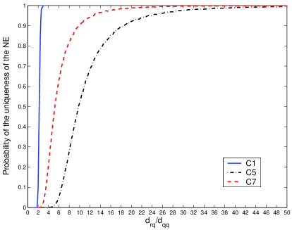
(a)  

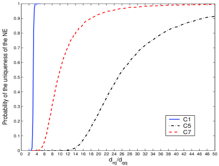
Figure 1: Probability of (C1), (C5) and (C7) versus $d_{rq}/d_{qq}$; $Q=5$ [subplot (a)], $Q=15$ [subplot (b)], $\gamma=2.5,$ $\Gamma_{q}=1,$ $d_{rq}/d_{qq}=d_{qr}/d_{rr},$ $\forall r,q\in\Omega,$ $N=64.$ 

We can see, from Figure 1, that the probability that the NE is unique increases as the links become more and more separated of each other (i.e., the ratio $d_{rq}/d_{qq}$ increases). Furthermore, we can verify that, even having not considered the smallest possible set $\mathcal{D}_{q}$, as defined in (27), our condition (C1) has a much higher probability of being satisfied than (C5) and (C7). The main difference between our condition (C1) and (C5), (C7) is that (C1) exhibits a neat threshold behavior since it transits very rapidly from the non-uniqueness guarantee to the almost certain uniqueness, as the inter-user distance ratio $d_{rq}/d_{qq}$ increases by a small amount. This shows that the uniqueness condition (C1) depends, ultimately, on the interlink distance rather than on the channel realization. This represents the fundamental difference between our uniqueness condition and those given in the literature. As an example, for a system with $Q=5$ links and probability $0.99$ of guaranteeing the uniqueness of the NE, condition (C1) requires $d_{rq}/d_{qq}\simeq 2$ whereas conditions (C5) and (C7) require $d_{rq}/d_{qq}>40$ and $d_{rq}/d_{qq}\simeq 24$, respectively. Furthermore, this difference increases as the number $Q$ of links increases.

5 Physical Interpretation of NE

In this section we provide a physical interpretation of the optimal power allocation corresponding to the NE in the limiting cases of low and high MUI. To quantify what low and high interference mean, we introduce the SNR of link $q$ (denoted by $\mathsf{snr}_{q}$) and the Interference-to-Noise Ratio due to the interference received by destination $q$ and generated by source $r,$ with $r\neq q$ (denoted by $\mathsf{inr}_{rq}$), defined as $\mathsf{snr}_{q}\triangleq P_{q}/(\sigma_{q}^{2}d_{qq}^{\alpha})$ and $\mathsf{inr}_{rq}\triangleq P_{r}/(\sigma_{q}^{2}d_{rq}^{\alpha}).$ Using $\mathsf{snr}_{q}$ and $\mathsf{inr}_{rq},$ the SINR $\mathsf{sinr}_{q}(k)$ in (23) can be rewritten as

$$\mathsf{sinr}_{q}(k)=\frac{\mathsf{snr}_{q}\left|\bar{H}_{qq}(k)\right|^{2}p_{q}(k)}{1+\sum_{\,r\neq q}\mathsf{inr}_{rq}\left|\bar{H}_{rq}(k)\right|^{2}p_{r}(k)}.$$ (30)

Low interference case.  Consider the low interference case, i.e., the situation where the interference term in the denominator in (30) can be neglected. A sufficient condition to satisfy this assumption is that the links are sufficiently far apart from each other, i.e., $d_{rq}>>d_{qq}$ $\forall r\neq q$,$r,q\in\Omega$. For sufficiently small $\mathsf{inr}_{rq}$ and sufficiently large $\mathsf{snr}_{q}$, condition (C1) is satisfied and, hence, by Theorem 1, the NE is unique. Also, by inspection of the waterfilling solution in (24), it is clear that under those conditions, $p_{q}(k)>0$ for all $q\in\Omega$ and $k\in\{1,\ldots,N\}$. This means that each source uses the whole bandwidth. Furthermore, it is well known that as the SNR increases, the waterfilling solution tends to a flat power allocation. In summary, we have the following result.

Proposition 1

Given game ${\mathscr{G}},$ there exist sets of values $\{\mathsf{inr}_{rq}^{\star}\}_{r\neq q\in\Omega}$ and $\{\mathsf{snr}_{q}^{\star}\}_{q\in\Omega},$ with $\mathsf{inr}_{rq}^{\star}<<1$ and $\mathsf{snr}_{q}^{\star}>>1,$ such that, for all $\mathsf{inr}_{rq}\leq\mathsf{inr}_{rq}^{\star}$ and $\mathsf{snr}_{q}\geq\mathsf{snr}_{q}^{\star},$ the NE of ${\mathscr{G}}$ is unique (cf. Theorem 2) and all users share the whole available bandwidth. In addition, if $\mathsf{snr}_{q}>>\mathsf{snr}_{q}^{\star},$ then the optimal power allocation of each user tends to be flat over the whole bandwidth.

From Proposition 1, it turns out, as it could have been intuitively guessed, that when the interference is low, at the (unique) NE, every user transmits over the entire available spectrum (like a CDMA system), as in such a case nulling the interference would not be worth of the bandwidth reduction. As a numerical example, in Figure 2, we plot the optimal power spectral density (PSD) of a system composed of three links, for different values of the ratio $d_{rq}/d_{qq}$. The results shown in Figure 2 have been obtained using the distributed algorithms described in Part II [32]. From Figure 2, we can check that, as the ratio $d_{rq}/d_{qq}$ increases, the optimal PSD tends to be flat, while satisfying the simultaneous waterfilling condition in (24).

High interference case. When $\mathsf{inr}_{rq}>>1$ for all $q$ and $r\neq q$, the interference is the dominant contribution in the equivalent noise (thermal noise plus MUI) in the denominator of (30). In this case, game ${\mathscr{G}}$ admits multiple Nash equilibria. An interesting class of these equilibria includes the FDMA solutions (called orthogonal Nash equilibria), occurring when the power spectra of different users are nonoverlapping. The characterization of these equilibria is given in the following.

Proposition 2

Given game ${\mathscr{G}},$ for each $q\in\Omega,$ let $\mathcal{I}_{q}\triangleq\left\{k\in\{1,\ldots,N\}:p_{q}(k)>0,\text{ }p_{r}(k)=0,\text{ }\forall r\right.$ $\left.\neq q\in\Omega\right\}$ denote the set of subcarriers over which only user $q$ transmits. For any given $\{\mathsf{snr}_{q}\}_{q\in\Omega},$ there exists $\{\mathsf{inr}_{rq}^{\star}\}_{r\neq q\in\Omega},$ with each $\mathsf{inr}_{rq}^{\star}>>1,$ such that for all $\mathsf{inr}_{rq}\geq\mathsf{inr}_{rq}^{\star}$, game ${\mathscr{G}}$ admits multiple orthogonal Nash equilibria. If, in addition, $\{\mathsf{snr}_{q}\}_{q\in\Omega}$ and $\{\mathsf{inr}_{rq}\}_{r\neq q\in\Omega}$ are such that

$$\Gamma_{q}\frac{\left|\bar{H}_{qr}(k)\right|^{2}}{\left|\bar{H}_{qq}(k)\right|^{2}}\frac{\mathsf{inr}_{qr}}{\mathsf{snr}_{q}}\leq 1,\quad k\in\mathcal{I}_{q},\text{ }r\neq q\in\Omega,$$ (31)

and an orthogonal NE still exists, the subcarriers are allocated among the users according to

$$\dfrac{\left|\bar{H}_{rr}(k_{r})\right|^{2}}{\left|\bar{H}_{qq}(k_{r})\right|^{2}}\geq\dfrac{\left|\bar{H}_{rr}(k_{q})\right|^{2}}{\left|\bar{H}_{qq}(k_{q})\right|^{2}},\qquad\text{ }k_{r}\in\mathcal{I}_{r}\text{ and }k_{q}\in\mathcal{I}_{q}.$$ (32)

Proof. See Appendix C.  

The above proposition has an intuitive interpretation: When the interference is very high, the users self-organize themselves in order to remove the interference totally, i.e., using nonoverlapping bands. In this case, game ${\mathscr{G}}$ may have multiple orthogonal Nash equilibria. For example, in the simple case of $Q=N,$ there are $Q!$ different orthogonal Nash equilibria, corresponding to all the permutations where each transmitter uses only one carrier. As the interference level decreases (i.e., the $\mathsf{inr}_{rq}$’s), the NE becomes unique and in such a case, if an orthogonal equilibrium still exists, then the distribution of the subcarriers among the users must satisfy the rule given by (32). This strategy is similar, in principle to FDMA, but differently from standard FDMA, here each user is getting the “best” portion of the spectrum for itself. Interestingly, (32) is the generalization of the condition satisfied by the subcarrier allocation in the multiple access frequency-selective channel, where the optimization problem is the sum-rate maximization under a transmit power constraint [39]. In Figure 2(b), we show a numerical example of the optimal power allocation at NE, for a system with two active links, in the case of high interference.

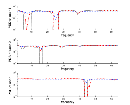
(a) Optimal PSDs at NE in the low-interference case.

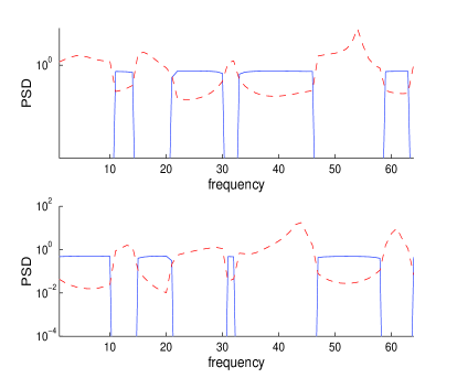
(b) Optimal PSDs at NE in the high-interference case.

Figure 2: Optimal PSDs at NE in the low-interference and high-interference cases: a) Solid, dashed, and dashed-dot line curves refer on the PSD obtained for $d_{rq}/d_{qq}=5,8$,$12$, respectively, and $\mathsf{snr}_{q}=15$ dB; b) Solid and dashed lines refer to PSD of each link and PSD of the MUI plus thermal noise, normalized by the channel transfer function square modulus of the link, respectively; $d_{12}/d_{22}=d_{21}/d_{11}=1,\Gamma_{1}=\Gamma_{2}=1,$ $\mathsf{snr}_{1}=\mathsf{snr}_{2}=5$ dB.

From Figure 2(b) we observe that, as predicted by Proposition 2, different users tend to transmit over non-overlapping bands.

In general, with intermediate interference levels, the optimal solution consists in allowing partial superposition of the PSDs of the users. An example of optimal PSD distribution for an intermediate level of interference is plotted in Figure 2(a) (see the curves obtained with $d_{rq}/d_{qq}=5$).

6 How good is a Nash Equilibrium ?

The optimality criterion used in this paper, based on the achievement of a NE, is useful to derive decentralized strategies. However, as the Nash equilibria need not to be Pareto-efficient [40], this criterion, in general, does not provide any a priori guarantee about the goodness of the equilibrium. Even when the equilibrium is unique, it is important to know how far is the performance from the optimal solution provided by a centralized strategy [12, 26]. The scope of this section is thus to quantify the performance loss resulting from the use of a decentralized approach, with respect to the optimal centralized solution. To this end, we compare the rates of the users corresponding to the Nash equilibria of game ${{\mathscr{G}}}$ in (20) with the rates lying on the boundary of the largest region of the achievable rates obtained as the Pareto-optimal trade-off surface solving the multi-objective optimization based on (21).

The rate region is defined as the set $\mathcal{R}$ of all feasible data rate combinations $\mathbf{r}\triangleq[r_{1},\ldots,r_{Q}]^{T}\in\mathcal{\mathbb{R}}_{+}^{Q}$ among the active links. A given vector of rates $\mathbf{r}\in\mathcal{\mathbb{R}}_{+}^{Q}$ is said to be feasible if it is possible to transfer information in the network at these rates, reliably, for some power allocation $\mathbf{p}\triangleq(\mathbf{p}_{q})_{q\in\Omega}$ satisfying the power constraints $\mathbf{p}_{q}\in{\mathscr{P}}_{q}$, $\forall q\in\Omega.$ The rate region can be numerically computed by considering all possible power allocations $\mathbf{p}$ such that $\mathbf{p}_{q}\in{\mathscr{P}}_{q}$, $\forall q\in\Omega$. Specifically, we have

$$\mathcal{R\ }\mathcal{=}\underset{\ \mathbf{p}_{q}\in{\mathscr{P}}_{q},\text{ }q\in\Omega}{\mathop{\displaystyle\bigcup}}\left\{\mathbf{r}\in\mathcal{\mathbb{R}}_{+}^{Q}\ |\ r_{q}\leq R_{q}(\mathbf{p}),\forall q\in\Omega\right\}=\left\{\mathbf{r}\in\mathcal{\mathbb{R}}_{+}^{Q}\ |\ \exists\ \mathbf{p}:\mathbf{p}_{q}\in{\mathscr{P}}_{q},\ r_{q}\leq R_{q}(\mathbf{p}),\ \forall q\in\Omega\right\}\vspace{-0.1cm}$$ (33)

where $R_{q}(\mathbf{p})$ and ${\mathscr{P}}_{q}$ are given in (21) and (22), respectively.

In general, the characterization of the rate region is a very difficult nonconvex optimization problem. Nevertheless, in the case of low interference, we have the following.

Proposition 3

In the case of low interference $(\mathsf{inr}_{rq}<<1),$ and high SNR $(\mathsf{snr}_{q}>>1),$ the rate region $\mathcal{R}$ given in (33) is a convex set.

Proof. See Appendix D.  

The best achievable trade-off among the rates is given by the Pareto optimal points of the set $\mathcal{R}$ given in (33). In formulas, all highest feasible rates can be found by solving the following multi-objective optimization problem (MOP) [11]:

$$\begin{array}[]{l}\mathop{\mathrm{m}aximize}\limits_{\mathbf{p}}\quad\text{\ }\left\{R_{1}(\mathbf{p}),\ldots,R_{Q}(\mathbf{p})\right\}\\ \text{subject to \quad\ }\mathbf{p}_{q}\in{\mathscr{P}}_{q},\quad\forall q\in\Omega.\end{array}$$ (34)

Practical algorithms to solve the MOP in (34) can be obtained, using the approach proposed, e.g., in [13, 42]. The Pareto optimal solutions to the MOP can also be obtained by solving the following ordinary scalar optimization:

$$\begin{array}[]{l}\mathop{\mathrm{m}aximize}\limits_{\mathbf{p}}\quad\ \ \ \sum\limits_{q=1}^{Q}\lambda_{q}R_{q}(\mathbf{p})\\ \text{subject to}\hskip 17.07182pt\ \mathbf{p}_{q}\in{\mathscr{P}}_{q},\quad\forall q\in\Omega.\end{array}$$ (35)

where $\boldsymbol{\lambda}$ is a set of positive weights. For any given $\boldsymbol{\lambda}>\mathbf{0},$ the (globally) optimal solution to (35) is a point on the trade-off surface of MOP (34) (cf. Appendix E). However, as the rate region (21) is in principle nonconvex, by varying $\boldsymbol{\lambda}>\mathbf{0,}$ only a portion of the trade-off curve of (34) can be explored. Specifically, all the Pareto optimal points lying on the nonconvex part of the rate region cannot be obtained as solutions to (35). We will refer to (35) as the scalarized MOP.

Comparing (20) with (34), we infer that, in general, the Nash equilibria are not solutions to (34), and thus they are not Pareto-efficient. An interesting question is whether one can modify the payoff function of every player so that some Nash equilibria of the modified game coincide with the Pareto optimal solutions. The answer is given by the following proposition.

Proposition 4

Let $\widetilde{{\mathscr{G}}}\left(\boldsymbol{\lambda}\right)$ be the game defined as

$$\widetilde{{\mathscr{G}}}\left(\boldsymbol{\lambda}\right)=\left\{\Omega,\left\{{\mathscr{P}}_{q}\right\}_{q\in\Omega},\{\widetilde{{\Phi}}_{q}\}_{q\in\Omega}\right\},$$ (36)

where the payoff functions are

$$\widetilde{{\Phi}}_{q}(\mathbf{p})={R}_{q}(\mathbf{p})+\frac{1}{\lambda_{q}}\sum_{r\neq q}\lambda_{r}{R}_{r}(\mathbf{p})\vspace{-0.2cm}$$ (37)

with $R_{q}(\mathbf{p})$ defined in (21) and $\boldsymbol{\lambda}\triangleq\mathbf{[}\lambda_{1},\ldots,\lambda_{Q}\mathbf{]}^{T}$ is a set of positive weights. Then, for any given $\boldsymbol{\lambda}>\mathbf{0}$, the solution set of $\widetilde{{\mathscr{G}}}(\boldsymbol{\lambda})$ is not empty and contains the (globally) optimal solution to the scalarized MOP (35), which is the Pareto optimal solution to the MOP (34) corresponding to the point where the hyperplane with normal vector $\boldsymbol{\lambda}$ is tangent to the boundary of the rate region (33).

Moreover, if the conditions of Proposition 3 are satisfied, then:

1. $\widetilde{{\mathscr{G}}}(\boldsymbol{\lambda})$ admits a unique NE, for any given $\boldsymbol{\lambda}>\mathbf{0},$ and

2. Any Pareto optimal solution to the MOP (34) can be obtained as the unique NE of $\widetilde{{\mathscr{G}}}(\boldsymbol{\lambda})$, with a proper choice of $\boldsymbol{\lambda}>\mathbf{0}.$

Proof. See Appendix E.  

Comparing (21) with (37), an interesting interpretation arises: The Pareto-optimal solutions to the MOP (34) can be achieved as a NE of the modified game where each player incorporates, in its utility function, a linear combination, through positive coefficient, of the utilities of the other players. The NE of the modified game $\widetilde{{\ \mathscr{G}}}(\boldsymbol{\lambda})$ in (36) can be obtained, for any given $\boldsymbol{\lambda},$ using, e.g., the gradient projection based iterative algorithm, proposed in [16]. However, this algorithm requires coordination among the players, since, at each iteration, each user has to know the channels and the strategies adopted by all the other users. Thus, Pareto-efficiency can be achieved only at the price of a significant increase of signalling and coordination among the users and this goes against our search for distributed, independent, coding/decoding among the users. Note that the structure of (37) generalizes the pricing techniques widely used in the game theory field to obtain a Pareto improvement of the system performance with respect to the Nash equilibria of a noncooperative game (see, e.g., [43] and references therein).

Using Proposition 4, we can now characterize and quantify the Nash equilibria of the game ${\mathscr{G}}$ given in (20) by providing upper and lower bounds.

Proposition 5

All the Nash equilibria $\mathbf{p}^{\star}$ of game ${\mathscr{G}}$ in (20) satisfy the following inequality

$$\max\limits_{\mathbf{p}_{q}\in{\mathscr{P}}_{q}}\min\limits_{\mathbf{p}_{-q}\in{\mathscr{P}}_{-q}}R_{q}(\mathbf{p}_{q},\mathbf{p}_{-q})\leq R_{q}(\mathbf{p}_{q}^{\star},\mathbf{p}_{-q}^{\star})\leq\widetilde{{\Phi}}_{q}^{\star},\quad\forall q\in\Omega,$$ (38)

where $\widetilde{{\Phi}}_{q}^{\star}$ is a NE of $\widetilde{{\mathscr{G}}}(\boldsymbol{\lambda})$ defined in (36) with a proper choice of $\boldsymbol{\lambda}.$

Proof. See Appendix F.  

Thus, at any NE of game ${\mathscr{G}}$ in (20), the rate of each user is always better than that obtained by optimizing the worst case (which in general is too pessimistic). However, in general, the Nash equilibria of ${\mathscr{G}}$ may be Pareto dominated. We quantify numerically this loss in the next section.

7 Numerical Results

It is interesting to compare the Nash equilibria of game ${\mathscr{G}}$ with the rates lying on the boundary of the rate region, in order to quantify the loss of Nash equilibria with respect to the Pareto optimal solutions. To this end, we consider the following two different topologies. In the first example, we assume that the system operates in a symmetric situation, whereas in the second example we consider an asymmetric scenario.

Example 1: Symmetric Case. In this scenario, the system is assumed to be symmetric, i.e., the transmitters have the same power budget and the interference links are at the same distance (i.e., $d_{rq}=d_{qr},\,\,\forall q,r$), so that the cross channel gains are comparable in average sense. In Figure 3, we plot the Pareto optimal points of  (34) and the Nash equilibria of game ${\mathscr{G}}$ defined in (20), for a two-users symmetric system. The two axes represent the rates, in bits/symbol, for the two links. The two pairs of nodes are placed at different distances, to test situations with different level of interference. In the picture, we plot: i) the Pareto-optimal boundary (33), referred to as $\mathcal{R}_{MOP}$ (solid lines); ii) the NE points ($\ast$) of game ${\mathscr{G},}$ given in (20); iii) the NE points of the modified game $\widetilde{{\mathscr{G}}}(\boldsymbol{\lambda}),$ given in (36), for different values of the vector $\boldsymbol{\lambda}$ (squares); and iv) the rate region (referred as $\mathcal{R}_{NE}$) corresponding to the Nash equilibria achieved by varying the transmit power of each link, under the constraint that the overall transmit power is fixed (dashed lines). All the Nash equilibria of game ${\mathscr{G}}$ are reached using the algorithms introduced in Part II of this paper [32], whereas the Nash equilibria of game $\widetilde{{\mathscr{G}}}(\boldsymbol{\lambda})$ are reached using the gradient projection algorithm, proposed in [16]. From Figure 3, we infer that the Nash equilibria approach the optimal Pareto curve as the interference level decreases (i.e., the ratio $d_{rq}/d_{qq}$ increases) at least in the two user case. This is not surprising as, in the case in which the interference is sufficiently low, the interaction (interference) among users becomes negligible and the performance is limited by noise only, not by the interference. On the contrary, at small interpair distances (i.e., small ratios $d_{rq}/d_{qq}$), interference becomes the dominant performance limiting factor and the loss resulting from using the decentralized approach becomes progressively larger. But the most interesting result is that this loss is limited also in the case where the links are rather close to each other (we have observed this result for several independent symmetric channel realizations). This suggests that, for symmetric systems, the decentralized approach, based on a game-theoretic formulation, is indeed a viable choice, considering its greater simplicity with respect to the centralized optimal solution. From Figure 3, we also see that the solutions to the MOP can be alternatively reached as Nash equilibria of the modified game $\widetilde{{\mathscr{G}}}$ in (36) (Proposition 4), using the gradient projection algorithm of [16]. However, this algorithm cannot be implemented in a distributed way, as it requires the knowledge from each user of the channels and the power allocations of all the other links.

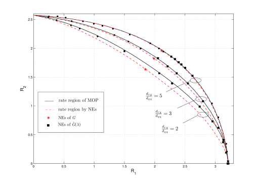
Figure 3: Rate region achieved for $d_{12}/d_{22}=d_{12}/d_{22}=2,3,5$, $d_{11}=d_{22}=1$, $P_{1}=P_{2}$, $\text{snr}_{1}=\text{snr}_{2}=10$ dB. Solid line, dashed line curves and asterisks refer on rate region given in (33), rate region obtained by NEs of $\widetilde{{\mathscr{G}}}(\boldsymbol{\lambda})$ given in (36), and NE points of game $\mathscr{G}$ given in (20), respectively.

Example 2: Asymmetric Case. We consider now a two-users system operating in an asymmetric situation, where one link receives a large interference whereas the other does not. This asymmetry can be due to many reasons, such as different transmission powers and/or unbalanced cross gains among the users (i.e., $d_{12}<<d_{21}$ or $d_{12}>>d_{21}$). For the sake of brevity, in the following we consider only the latter case, i.e., the situation in which both transmitters have the same power budget but, because of the location of transmitters and receivers, one link receives much more interference than the other. In Figure 4(a) we plot the Pareto optimal points of  (34) and the Nash equilibria of game ${\mathscr{G}}$ defined in (20), for a two-users asymmetric system, for different values of the ratio $d_{12}/d_{21}$ and a given channel realization. Low values of $d_{12}/d_{21}$ correspond to high asymmetric situations. From the figure we infer that as the asymmetry of the system increases (i.e., $d_{12}/d_{21}$ decreases) the loss of Nash equilibria with respect to the corresponding Pareto optimal points becomes more significant. As an example, for the setup considered in the figure, the performance loss in terms of sum-rate can be as large as $30\%$ of the globally optimal solution. The same qualitative behavior has been observed changing the channel realizations and the number of users.

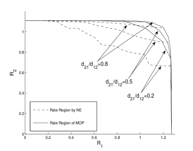
(a)  

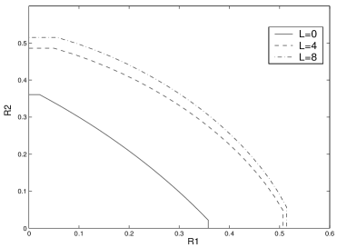
Figure 4: a) Rate region achieved in the asymmetric case, for $d_{12}/d_{21}=0.2,0.5,0.8$, $d_{11}=d_{22}=1$, $P_{1}=P_{2}$, $\text{snr}_{1}=\text{snr}_{2}=5$ dB. Solid line and dashed line curves refer on rate region given in (33) and rate region obtained by NEs of $\mathscr{G}$ given in (20), respectively; b) Rate region achieved for $L=0,4,8$, $N=64$, $d_{12}/d_{22}=d_{21}/d_{11}=1$, $d_{11}=d_{22}=1$, $P_{1}=P_{2}$, $\text{snr}_{1}=\text{snr}_{2}=5$ dB.

Example 3: Rate region versus channel order. Finally, we study the effect of channel frequency selectivity on the Nash equilibria of game ${\mathscr{G}}$ in (20). To this end, we plot in Figure 4 the average rate region obtained by the Nash equilibria of ${\mathscr{G}}$ for different values of the channel order $L_{h}$. The channel taps are simulated as i.i.d. Gaussian random variables with zero mean and variance $1/(L_{h}+1)$. From the figure, we infer that the performance of decentralized system improves with the channel order. This is due to the fact that larger frequency fluctuations of the channel provide more degrees of freedom for each user to find out the best spectral partition for itself, given its own channel and interference.

8 Conclusions

In this paper we formulated the problem of finding the optimal precoding/multiplexing strategy in an infrastructureless multiuser scenario as a noncooperative game. We first considered the theoretical problem of maximizing mutual information on each link, given constraints on the spectral mask and transmit power. Then, to accommodate practical implementation aspects, we focused on the competitive maximization of the transmission rate on each link, using finite order constellations, under the same constraints as above plus a constraint on the average error probability. We proved that in both cases a NE always exists and the optimal precoding/multiplexing strategy leads to a (pure strategy) diagonal transmission for all the users. This result strongly simplifies the optimization, as we can reduce both original complicated matrix-valued games to a simpler unified vector power control game. Thus, we studied such a game, and derived sufficient conditions for the uniqueness of the NE, that were proved to have a broader validity than the conditions known in the literature for special cases of our game. Then, we compared the totally decentralized strategy with the Pareto-optimal centralized solution and we observed that the decentralized strategy has rather low performance loss with respect to the Pareto-optimal solution, especially for symmetric systems. Larger losses were observed in the case of very asymmetric systems.  In the effort to approach the Pareto-optimal performance, we then showed how to modify the payoff of each user in order to create a modified game, whose Nash equilibria are Pareto-optimal. However, this comes at the cost of extra signaling among the users and breaks the noncooperative feature of the original games.

Once proved that a Nash equilibrium exists and under which conditions is unique, the problem boils down to how to reach such an equilibrium. This problem is addressed in Part II of this paper [32], where we provide a variety of distributed algorithms along with their convergence conditions.

Appendix A Proof of Theorem 1

We first prove Theorem 1 for game $\mathscr{G}_{1}.$ Then, we show that the same result holds true also for game $\mathscr{G}_{2}.$

A.1 Game $\mathscr{G}_{1}$

Given $\mathscr{G}_{1}$ in (9), according to the definition of NE (cf. Definition 1), the proof consists in showing that for each player $q,$ given the optimal strategy profiles of the others at some NE (corresponding to the optimal matrices $\mathbf{F}_{r}=\mathbf{W\Sigma}_{r}^{1/2},$ with $\mathbf{\Sigma}_{r}\triangleq\mathop{\mathrm{d}iag}(\mathbf{p}_{r}),$ $\forall r\neq q$) i.e., $\mathbf{R}_{-q}=\sigma_{q}^{2}\mathbf{I}+\sum\limits_{r\neq q\hfill\hfill}\mathbf{H}_{rq}\mathbf{W\Sigma}_{r}\mathbf{W}^{H}\mathbf{H}_{rq}^{H}$, the maximum of mutual information ${\mathop{\mathrm{I}}\nolimits_{q}}(\mathbf{F}_{q},\mathbf{F}_{-q})$ defined in (7), under constraints (10), is achieved by $\mathbf{F}_{q}\mathbf{F}_{q}^{H}=\mathbf{W\Sigma}_{q}\mathbf{W}^{H},$ where $\mathbf{\Sigma}_{q}\triangleq\mathop{\mathrm{d}iag}(\mathbf{p}_{q})$ and $\mathbf{p}_{q}$ is solution to (20), for fixed $\mathbf{p}_{-q}.$

In the absence of spectral mask constraints, the statement of the theorem comes directly from the well-known diagonality result of the capacity-achieving solution to the single user vector Gaussian channel [34], and the fact that all channel matrices in (7) are diagonalized by the IFFT matrix $\mathbf{W}$:

$$\log\left(\left|\mathbf{I}+\mathbf{F}_{q}^{H}\mathbf{H}_{qq}^{H}\mathbf{R}_{\mathbf{-}q}^{-1}\mathbf{H}_{qq}\mathbf{F}_{q}\right|\right)=\log\left(\left|\mathbf{I}+\mathbf{\Lambda}_{q}\mathbf{Q}_{q}\right|\right)\leq\sum_{k}\log\left(1+\left[\mathbf{\Lambda}_{q}\right]_{kk}\left[\mathbf{Q}_{q}\right]_{kk}\right),\vspace{-0.2cm}$$ (39)

where $\mathbf{Q}_{q}\triangleq\mathbf{W}^{H}\mathbf{F}_{q}\mathbf{F}_{q}^{H}\mathbf{W,}$ we have used the eigen-decomposition $\mathbf{H}_{qq}^{H}\mathbf{R}_{\mathbf{-}q}^{-1}\mathbf{H}_{qq}=\mathbf{W\Lambda}_{q}\mathbf{W}^{H},$ with

$$\left[\mathbf{\Lambda}_{q}\right]_{kk}=\frac{\left|H_{qq}(k)\right|^{2}}{1+\sum_{\,r\neq q}\left|H_{rq}(k)\right|^{2}p_{r}(k)},\quad k\in\{1,\ldots,N\},$$ (40)

and the last inequality follows from the Hadamard’s inequality [34]. Since the equality in (39) is reached if and only if $\mathbf{Q}_{q}$ is diagonal and the power constraint $\mathsf{Tr}\left(\mathbf{F}_{q}\mathbf{F}_{q}^{H}\right)=\mathsf{Tr}\left(\mathbf{Q}_{q}\right)\leq P_{T}$ depends only on the diagonal elements of $\mathbf{Q}_{q},$ we may set $\mathbf{Q}_{q}$ diagonal w.l.o.g., i.e., $\mathbf{Q}_{q}=\mathbf{\Sigma}_{q};$ which leads to the desired optimal structure for $\mathbf{F}_{q}$.

Interestingly, in the presence of spectral mask constraints, we can still use the previous result since the additional constraints $\left[\mathbf{W}^{H}\mathbf{F}_{q}\mathbf{F}_{q}^{H}\mathbf{W}\right]_{kk}=\left[\mathbf{Q}_{q}\right]_{kk}\leq\overline{p}_{q}^{\max}(k)$ depend only on the diagonal elements of $\mathbf{Q}_{q}.$ Introducing the optimal structure $\mathbf{F}_{q}=\mathbf{W\Sigma}_{q}^{1/2}$ in $\mathscr{G}_{1}$, we obtain the simpler game $\mathscr{G}$ in (20).

A.2 Game $\mathscr{G}_{2}$

The proof hinges on majorization theory for which the reader is referred to [44] or [8, 45]. The key definitions and results on which the proof is based are outlined next for convenience.

Definition 2 ([44, $1.A.1$])

For any two vectors $\mathbf{x},\mathbf{y\in\mathbb{R}}^{n}$, we say $\mathbf{x}$ is majorized by $\mathbf{y}$ or  $\mathbf{y}$ majorizes $\mathbf{x}$ (denoted by $\mathbf{x}\prec\mathbf{y}$ or $\mathbf{y\succ x}$) if

$$\sum_{k=1}^{i}x_{[k]} \leq \sum_{k=1}^{i}y_{[k]},\quad 1\leq k<n,$$

$$\sum_{k=1}^{n}x_{[k]} = \sum_{k=1}^{n}y_{[k]},$$

where $x_{[k]}$ and $y_{[k]}$ denote the elements of $\mathbf{x}$ and $\mathbf{y}$, respectively, in decreasing order.

Definition 3

A real valued function $\phi$ defined on a set $\mathcal{A}\subseteq\mathbb{R}^{n}$ is said to be Schur-convex on $\mathcal{A}$ if

$$\mathbf{x}\prec\mathbf{y\quad}\text{on }\mathcal{A}\text{ }\mathbf{\quad\Rightarrow\quad}\phi(\mathbf{x})\leq\phi(\mathbf{y}).$$ (41)

Similarly, $\phi$ is said to be Schur-concave on $\mathcal{A}$ if

$$\mathbf{x}\prec\mathbf{y\quad}\text{on }\mathcal{A}\text{ }\mathbf{\quad\Rightarrow\quad}\phi(\mathbf{x})\geq\phi(\mathbf{y}).$$ (42)

Lemma 1 ([44, p.7], [44, 9.B.1])

For a Hermitian matrix $\mathbf{A}$ and a unitary matrix $\mathbf{U,}$ it follows that

$$\mathbf{1}(\mathbf{A})\prec\mathbf{d}(\mathbf{U}^{H}\mathbf{AU})\prec\boldsymbol{\lambda}(\mathbf{A})\mathbf{,}$$ (43)

where $\mathbf{d}(\mathbf{A})$ and $\boldsymbol{\lambda}(\mathbf{A})$ denote the diagonal elements and eigenvalues of $\mathbf{A},$ respectively, and $\mathbf{1}$ denotes the vector with identical components equal to the average of the diagonal elements of $\mathbf{A}$.

Interestingly, matrix $\mathbf{U}$ in (43) can always be chosen such that the diagonal elements are equal to one extreme or the other. To achieve $\mathbf{d}(\mathbf{U}^{H}\mathbf{AU})=\mathbf{1}(\mathbf{A}),$ $\mathbf{U}$ has to be chosen such that $\mathbf{U}^{H}\mathbf{AU}$ has equal diagonal elements; to achieve $\mathbf{d}(\mathbf{U}^{H}\mathbf{AU})=\boldsymbol{\lambda}(\mathbf{A}),$ $\mathbf{U}$ has to be chosen to diagonalize matrix $\mathbf{A},$ i.e., equal to the eigenvectors of $\mathbf{A}.$

As in Appendix A.1, the proof consists in showing that, given the optimal strategy profiles of the others at some NE, the optimal precoding matrix of user $q$, solution to (18), is in the form of (19).  Thus, hereafter we can focus on a generic user $q,$ and assume that the strategy profiles of the others are fixed and equal to $\mathbf{F}_{r}=\mathbf{W\Sigma}_{r}^{1/2},$ with $\mathbf{\Sigma}_{r}\triangleq\mathop{\mathrm{d}iag}(\mathbf{p}_{r}),$ $\forall r\neq q.$ We prove the theorem in two steps. Given $q,$ first, we show the equivalence of the original complicated problem (18) and a simpler problem, and then, we solve the simple problem, implying the optimality of $\mathbf{F}_{q}$ in the form (19).

Defining $\mathbf{P}_{q}\triangleq\mathbf{W}^{H}\mathbf{F}_{q},$ the MSE matrix of user $q$ can be written as

$$\mathbf{E}_{q}\mathbf{(P}_{q}\mathbf{)}\triangleq(\mathbf{I+F}_{q}^{H}\mathbf{H}_{qq}^{H}\mathbf{R}_{q}^{-1}\mathbf{H}_{qq}\mathbf{F}_{q})^{-1}=(\mathbf{I+F}_{q}^{H}\mathbf{W\Lambda}_{q}\mathbf{W}^{H}\mathbf{F}_{q})^{-1}=(\mathbf{I+P}_{q}^{H}\mathbf{\Lambda}_{q}\mathbf{P}_{q})^{-1},$$ (44)

where in the second equality we used $\mathbf{R}_{-q}=\sigma_{q}^{2}\mathbf{I}+\sum\limits_{r\neq q\hfill\hfill}\mathbf{H}_{rq}\mathbf{W\Sigma}_{r}\mathbf{W}^{H}\mathbf{H}_{rq}^{H}$ and the eigen-decomposition $\mathbf{H}_{qq}^{H}\mathbf{R}_{\mathbf{-}q}^{-1}\mathbf{H}_{qq}=\mathbf{W\Lambda}_{q}\mathbf{W}^{H},$ with $\mathbf{\Lambda}_{q}$ defined in (40). The matrix $\mathbf{E}_{q}\mathbf{(P}_{q}\mathbf{)}$ has the following properties: i) $\mathbf{E}_{q}\mathbf{(P}_{q}\mathbf{)}$ is a continuous function of $\mathbf{P}_{q}\in\mathbb{C}^{N\times N}$; ii) For any unitary matrix $\mathbf{U},$ $\mathbf{E}_{q}\mathbf{(P}_{q}\mathbf{)}$ satisfies

$$\mathbf{E}_{q}\mathbf{(P}_{q}\mathbf{U)=U}^{H}\mathbf{E}_{q}\mathbf{(P}_{q}\mathbf{)U.}$$ (45)

Using (44), the payoff function of user $q$ (to be minimized) in (18) can be written as a function of $\mathbf{d}(\mathbf{E}_{q}\mathbf{(P}_{q}\mathbf{))}$:

$$f_{q}(\mathbf{d}(\mathbf{E}_{q}\mathbf{(P}_{q}\mathbf{)}))\triangleq-\mathop{\mathrm{r}}\nolimits_{q}(\mathbf{F}_{q})=-\frac{1}{N}\mathop{\displaystyle\sum}\limits_{k=1}^{N}\log_{2}\left(1\mathcal{+}\frac{\left(\left[\mathbf{E}_{q}\mathbf{(P}_{q}\mathbf{)}\right]_{kk}\right)^{-1}-1}{\Gamma_{q}}\right),\vspace{-0.3cm}$$ (46)

where $\mathop{\mathrm{r}}\nolimits_{q}(\mathbf{F}_{q})$ is defined in (17) and the last equality follows from the relation $\mathop{\mathrm{S}INR}\nolimits_{k,q}(\mathbf{F}_{q})=\left(\left[\mathbf{E}_{q}\mathbf{(P}_{q}\mathbf{)}\right]_{kk}\right)^{-1}$ $-1,$ with $\mathop{\mathrm{S}INR}\nolimits_{k,q}(\mathbf{F}_{q})$ defined in (16).  The function $f_{q}$ has the following properties: i) $f_{q}(\mathbf{d}(\mathbf{E}_{q}\mathbf{(P}_{q}\mathbf{)}))$ is a continuous function of $\mathbf{P}_{q}\in\mathbb{C}^{N\times N}$ (implied from the continuity of $\mathbf{E}_{q}\mathbf{(P}_{q}\mathbf{),}$ as pointed out before); ii) $f_{q}(\mathbf{d}(\mathbf{E}_{q}\mathbf{(P}_{q}\mathbf{)}))$ is a Schur-concave function on $\mathbb{R}_{+}^{N}$ (cf. Definition 3) [9].

Using (44) and (46), the optimization problem of user $q$ in (18) becomes

$$\begin{array}[]{ll}\mathop{\mathrm{m}inimize}\limits_{\mathbf{P}_{q}}&f_{q}(\mathbf{d}(\mathbf{E}_{q}\mathbf{(P}_{q}\mathbf{)}))\\ \mathop{\mathrm{s}ubject}\text{ }\mathop{\mathrm{t}o}&\begin{array}[]{l}\dfrac{1}{N}\mathsf{Tr}\left(\mathbf{P}_{q}\mathbf{P}_{q}^{H}\right)\leq P_{q},\\ \mathbf{d}\left(\mathbf{P}_{q}\mathbf{P}_{q}^{H}\right)\leq\overline{\mathbf{p}}_{q}^{\max},\end{array}\end{array}$$ (P1)

where $\overline{\mathbf{p}}_{q}^{\max}\triangleq(\overline{p}_{q}^{\max}(k))_{k=1}^{N}.$ Observe that problem P1 always admits a solution, since the feasible set is closed and bounded (thus compact) and the objective function is continuous in its interior (as pointed out before). A priori the solution is unknown, but we assume it given by an oracle and denoted by $\mathbf{P}_{q}^{\star}$. As it will be shown next, we do not need to know explicitly such a solution to complete the proof of the theorem. Then, problem P1 is equivalent to

$$\begin{array}[]{ll}\mathop{\mathrm{m}inimize}\limits_{\mathbf{P}_{q}}&f_{q}(\mathbf{d}(\mathbf{E}_{q}\mathbf{(P}_{q}\mathbf{)}))\\ \mathop{\mathrm{s}ubject}\text{ }\mathop{\mathrm{t}o}&\mathbf{d}\left(\mathbf{P}_{q}\mathbf{P}_{q}^{H}\right)=\mathbf{d}_{q}^{\star},\end{array}$$ (P2)

where $\mathbf{d}_{q}^{\star}\triangleq\mathbf{d}\left(\mathbf{P}_{q}^{\star}\mathbf{P}_{q}^{\star H}\right).$ The equivalence of both problems is in the following sense: 1) The optimal (and thus feasible) point $\mathbf{P}_{q}^{\star}$ of P1 is feasible in P2 with the same value of the objective function; 2)  A feasible point in P2 (not necessarily optimal) is feasible also in P1 with the same value of the objective function.

Thus, for any given $\mathbf{d}_{q}^{\star},$ we can focus on solving problem P2 w.l.o.g., and show that the optimal solution to P2 is diagonal; which leads to the desired structure for the original matrix $\mathbf{F}_{q}$ in (18). Since $f_{q}\left(\mathbf{d}\left(\mathbf{E}_{q}(\mathbf{P}_{q})\right)\right)$ is Schur-concave, it follows from Definition 3 and Lemma 1 that $f_{q}\left(\mathbf{d}\left(\mathbf{E}_{q}(\mathbf{P}_{q})\right)\right)\geq f_{q}\left(\boldsymbol{\lambda}\left(\mathbf{E}_{q}(\mathbf{P}_{q})\right)\right).$ Interestingly, for any given $\mathbf{P}_{q}$, it is always possible to achieve the lower bound $f_{q}\left(\boldsymbol{\lambda}\left(\mathbf{E}_{q}(\mathbf{P}_{q})\right)\right)$ of $f_{q}\left(\mathbf{d}\left(\mathbf{E}_{q}(\mathbf{P}_{q})\right)\right)$ by using instead the matrix $\widetilde{\mathbf{P}}_{q}=\mathbf{P}_{q}\mathbf{U}$ such that $\mathbf{E}_{q}(\widetilde{\mathbf{P}}_{q})=\mathbf{U}^{H}\mathbf{E}_{q}\mathbf{(P}_{q}\mathbf{)U}$ is diagonal (see (45)), without affecting the constraints, since $\mathbf{d}(\widetilde{\mathbf{P}}_{q}\widetilde{\mathbf{P}}_{q}^{H})=\mathbf{d}\left(\mathbf{P}_{q}\mathbf{P}_{q}^{H}\right).$ In such a case, $f_{q}(\mathbf{d}(\mathbf{E}_{q}(\widetilde{\mathbf{P}}_{q})))=f_{q}(\boldsymbol{\lambda}(\mathbf{E}_{q}(\widetilde{\mathbf{P}}_{q})))=f_{q}\left(\mathbf{d}\left(\mathbf{E}_{q}(\mathbf{P}_{q})\right)\right).$ This implies that there is an optimal $\mathbf{P}_{q}$ for problem P2 such that $\mathbf{E}_{q}(\mathbf{P}_{q})$ is diagonal or, equivalently from (44), such that $\mathbf{P}_{q}^{H}\mathbf{\Lambda}_{q}\mathbf{P}_{q}$ is diagonal.

Now, given that $\mathbf{P}_{q}^{H}\mathbf{\Lambda}_{q}\mathbf{P}_{q}$ is a diagonal matrix, let us say $\mathbf{\Sigma}_{q},$ i.e., $\mathbf{P}_{q}^{H}\mathbf{\Lambda}_{q}\mathbf{P}_{q}=$ $\mathbf{\Sigma}_{q}$, we can write $\mathbf{P}_{q}$ as $\mathbf{P}_{q}=\mathbf{\Lambda}_{q}^{-1/2}\mathbf{U}_{q}\mathbf{\Sigma}_{q}^{1/2}$ w.l.o.g. (see, e.g., [8, 45]), where $\mathbf{U}_{q}$ is any unitary matrix. Using such a structure of $\mathbf{P}_{q},$ problem P1 can be equivalently written as

$$\begin{array}[]{ll}\mathop{\mathrm{m}inimize}\limits_{\mathbf{\Sigma}_{q}\mathbf{,U_{q}}}&-\mathop{\displaystyle\sum}\limits_{k=1}^{N}\log_{2}\left(1\mathcal{+}\dfrac{\left[\mathbf{\Sigma}_{q}\right]_{kk}}{\Gamma_{q}}\right)\\ \mathop{\mathrm{s}ubject}\text{ }\mathop{\mathrm{t}o}&\mathbf{d}\left(\mathbf{U}_{q}\mathbf{\Sigma}_{q}\mathbf{U}_{q}^{H}\right)=\overline{\mathbf{d}}_{q}^{\star},\end{array}$$ (47)

where $\overline{\mathbf{d}}_{q}^{\star}\triangleq\mathbf{\Lambda}_{q}\mathbf{d}^{\star}$.

From majorization theory (see [44, 5.A.9.A and 9.B.2] or [45, Lemma 4 and Lemma 3]) we know that, for any given $\mathbf{\Sigma}_{q},$ we can always find a unitary matrix $\mathbf{U}_{q}$ satisfying the constraint in (47) if and only if

$$\boldsymbol{\lambda}(\mathbf{\Sigma}_{q})\succ\overline{\mathbf{d}}_{q}^{\star}.$$ (48)

Therefore, we can first find the optimal $\mathbf{\Sigma}_{q}$ in (47) replacing the original constraint with (48) and then choose the matrix $\mathbf{U}_{q}$ to satisfy the constraint in (47) with that optimal $\mathbf{\Sigma}_{q}.$ Therefore, we have

$$\begin{array}[]{ll}\mathop{\mathrm{m}inimize}\limits_{\mathbf{\Sigma}_{q}}&-\mathop{\displaystyle\sum}\limits_{k=1}^{N}\log_{2}\left(1\mathcal{+}\dfrac{\left[\mathbf{\Sigma}_{q}\right]_{kk}}{\Gamma_{q}}\right)\\ \mathop{\mathrm{s}ubject}\text{ }\mathop{\mathrm{t}o}&\mathbf{d}\left(\mathbf{\Sigma}_{q}\right)\succ\overline{\mathbf{d}}_{q}^{\star}.\end{array}$$ (49)

Since the objective function in (49) is Schur-convex, it follows from Definition 3 that the optimal solution $\mathbf{\Sigma}_{q}^{\star}$ to (49) is $\mathbf{d}\left(\mathbf{\Sigma}_{q}^{\star}\right)=\overline{\mathbf{d}}_{q}^{\star}.$ Given such a $\mathbf{\Sigma}_{q}^{\star},$ the constraint in (47) is satisfied if the matrix $\mathbf{U}_{q}\mathbf{=I}$, implying for $\mathbf{P}_{q}$ in problem P2 the optimal structure $\mathbf{P}_{q}=$ $\mathbf{\Lambda}_{q}^{-1/2}\mathbf{\Sigma}_{q}^{1/2};$ which leads to the desired expression for $\mathbf{F}_{q}=\mathbf{WP}_{q}=\mathbf{W\Lambda}_{q}^{-1/2}\mathbf{\Sigma}_{q}^{1/2}\triangleq\mathbf{W}\sqrt{\mathop{\mathrm{d}iag}(\mathbf{p}_{q})}.$This proves that all the solutions to problem P1 can be obtained using $\mathbf{F}_{q}=\mathbf{W}\sqrt{\mathop{\mathrm{d}iag}(\mathbf{p}_{q})}.$ 

Appendix B Proof of Theorem 2

B.1 Existence of a NE

First, we show the existence of NE for the game ${\ \mathscr{G}}$ in (20) using the following fundamental game theory result:

Theorem 3

[14, 16] The strategic noncooperative game ${\mathscr{G}}=\left\{\Omega,\{\mathcal{X}_{q}\}_{q\in\Omega},\{{\Phi}_{q}\}_{q\in\Omega}\right\}$ admits at least one NE if, for all $q\in\Omega$: $1)$ The set $\mathcal{X}_{q}$ is a nonempty compact convex subset of a Euclidean space, and $2)$ The payoff function $\Phi_{q}(\mathbf{x})$ is continuous on $\mathcal{X}$ and quasi-concave on $\mathcal{X}_{q}$.

The game $\mathscr{G}$ in (20) always admits at least one NE, because it satisfies conditions required by Theorem 3: $1)$ The set ${\mathscr{P}}_{q}$ of feasible strategy profiles, given by (22), is convex and compact (because it is closed and bounded); $2)$ The payoff function of each player $q$ in (20) is continuous in $\mathbf{p}$ and (strict) concave in $\mathbf{p}_{q}\in{\mathscr{P}}_{q}$ for any given $\mathbf{p}_{-q}$ (this follows from the concavity of the log function). Hence, it is also quasi-concave [33].

B.2 Uniqueness of the NE

To prove the uniqueness we need the following intermediate results.

Definition 4

A matrix $\mathbf{A}\in\mathbb{R}^{n\times n}$ is said to be a $\mathbf{Z}$-matrix if its off-diagonal entries are all non-positive. A matrix $\mathbf{A}\in\mathbb{R}^{n\times n}$ is said to be a $\mathbf{P}$-matrix if all its principal minors are positive. A $\mathbf{Z}$-matrix which is also $\mathbf{P}$ is called a $\mathbf{K}$-matrix.

Many equivalent characterizations for the above classes of matrices can be given. The interested reader is referred to [48, 49] for more details. Here we focus on the following two properties.

Lemma 2 ([48, Theorem $3.3.4$])

A matrix $\mathbf{A}\in\mathbb{R}^{n\times n}$ is a $\mathbf{P}$-matrix if and only if $\ \mathbf{A}$ does not reverse the sign of any nonzero vector, i.e.,

$$x_{i}\left[\mathbf{Ax}\right]_{i}\leq 0\text{ \ for all }i\text{ \ }\Rightarrow\text{ \ }\mathbf{x=0}\text{.}$$ (50)

Lemma 3 ([48, Lemma $5.3.14$])

Let $\mathbf{A}\in\mathbb{R}^{n\times n}$ be a $\mathbf{K}$-matrix and $\mathbf{B}$ a nonnegative matrix. Then $\rho(\mathbf{A}^{-1}\mathbf{B})<1$ if and only if $\mathbf{A-B}$ is a $\mathbf{K}$-matrix.

We provide now sufficient conditions for the uniqueness of the NE. First, we derive a necessary condition for two admissible strategy profiles (whose existence is guaranteed by the first part of the Theorem) to be different Nash equilibria of the game ${\mathscr{G}}$ in (20). Then we obtain a simple sufficient condition that guarantees the previous condition is not satisfied; hence guaranteeing that there cannot be two different Nash equilibria.

Assume that the game ${\mathscr{G}}$ admits two distinct NE points, denoted by $\mathbf{p}^{(0)},\mathbf{p}^{(1)},$ where $\mathbf{p}^{(r)}\triangleq[\mathbf{p}_{1}^{(r)T},\ldots,\mathbf{p}_{Q}^{(r)T}]^{T}$ and $\mathbf{p}_{q}^{(r)}\triangleq[p_{q}^{(r)}(1),\ldots,p_{q}^{(r)}(N)]^{T},$ with $r=0,1,$ $q\in\Omega.$ Then, they must satisfy the following (necessary and sufficient) Karush-Kuhn-Tucker (KKT) conditions (see, e.g., [33]) for each $q\in\Omega$:

$$\begin{array}[]{l}\nabla_{\mathbf{p}_{q}}R_{q}\left(\mathbf{p}^{\left(r\right)}\right)+\mathop{\displaystyle\sum}\limits_{k=1}^{2N+1}\mu_{q,k}^{\left(r\right)}\nabla_{\mathbf{p}_{q}}f_{q,k}(\mathbf{p}_{q}^{\left(r\right)})=\mathbf{0},\vskip 6.0pt plus 2.0pt minus 2.0pt\\ \mu_{q,k}^{\left(r\right)}f_{q,k}(\mathbf{p}_{q}^{\left(r\right)})=0,\ \mathbf{\boldsymbol{\mu}}_{q}^{r}\geq\mathbf{0},\ f_{q,k}(\mathbf{p}_{q}^{\left(r\right)})\geq 0,\end{array}\qquad\text{ }r=0,1,\vspace{-0.2cm}$$ (51)

where $\mathbf{\boldsymbol{\mu}}_{q}^{\left(r\right)}\triangleq[\mu_{q,1}^{\left(r\right)},\ldots,\mu_{q,2N+1}^{\left(r\right)}]^{T}$ is the nonnegative Lagrange multiplier vector, and

$$\begin{array}[]{l}f_{q,k}(\mathbf{p}_{q}^{\left(r\right)})=\left\{\begin{array}[]{ll}p_{q}^{\left(r\right)}(k),&\text{if }1\leq k\leq N,\\ 1-\mathbf{1}^{T}\mathbf{p}_{q}^{\left(r\right)},&\text{if \ }k=N+1,\\ p_{q}^{\max}(k-N-1)-p_{q}^{(r)}(k-N-1),&\text{if }N+1<k\leq 2N+1,\end{array}\right.\\ \left[\nabla_{\mathbf{p}_{q}}R_{q}\left(\mathbf{p}\right)\right]_{k}=\dfrac{\log e}{\Gamma_{q}N}\dfrac{\left|H_{qq}(k)\right|^{2}}{1+\sum_{r\neq q,r=1}^{Q}\left|H_{rq}(k)\right|^{2}p_{r}(k)+\Gamma_{q}^{-1}\left|H_{qq}(k)\right|^{2}p_{q}(k)}\vskip 3.0pt plus 1.0pt minus 1.0pt\\ \hskip 64.01869pt=\dfrac{\log e}{\Gamma_{q}N}\dfrac{|H_{qq}(k)|^{2}}{1+\sum_{r=1}^{Q}\Gamma_{q}^{-\delta_{rq}}|H_{rq}(k)|^{2}p_{r}(k)},\vskip 6.0pt plus 2.0pt minus 2.0pt\end{array}$$ (52)

with $\delta_{rq}$ defined as $\delta_{rq}=1$ if $r=q$ and $\delta_{rq}=0$ otherwise. Note that the functions $f_{q,k}(\mathbf{p}_{q}^{\left(r\right)})$ are (linear) concave, thus it must be that, for each $\mathbf{p}_{q}^{(1)}$ and $\mathbf{p}_{q}^{(0)},$ [33]

$$f_{q,k}(\mathbf{p}_{q}^{\left(1\right)})\leq f_{q,k}(\mathbf{p}_{q}^{\left(0\right)})+\left(\mathbf{p}_{q}^{(1)}-\mathbf{p}_{q}^{(0)}\right)^{T}\nabla_{\mathbf{p}_{q}}\text{ }f_{q,k}(\mathbf{p}_{q}^{\left(0\right)}),\quad\forall k\in\{1,\ldots,2N+1\},\quad\forall q\in\Omega.$$ (53)

Multiplying the first equation of (51) by $\left(\mathbf{p}_{q}^{(1)}-\mathbf{p}_{q}^{(0)}\right)^{T}$ for $r=0,$ by $\left(\mathbf{p}_{q}^{(0)}-\mathbf{p}_{q}^{(1)}\right)^{T}$ for $r=1,$ and summing over $r$ we obtain, for each $q\in\Omega:$

$$\begin{array}[]{l}\left(\mathbf{p}_{q}^{(1)}-\mathbf{p}_{q}^{(0)}\right)^{T}\nabla_{\mathbf{p}_{q}}R_{q}\left(\mathbf{p}^{\left(0\right)}\right)+\left(\mathbf{p}_{q}^{(0)}-\mathbf{p}_{q}^{(1)}\right)^{T}\nabla_{\mathbf{p}_{q}}R_{q}\left(\mathbf{p}^{\left(1\right)}\right)+\\ \mathop{\displaystyle\sum}\limits_{k=1}^{2N+1}\left[\mu_{q,k}^{\left(0\right)}\left(\mathbf{p}_{q}^{(1)}-\mathbf{p}_{q}^{(0)}\right)^{T}\nabla_{\mathbf{p}_{q}}f_{q,k}(\mathbf{p}_{q}^{\left(0\right)})+\mu_{q,k}^{1}\left(\mathbf{p}_{q}^{(0)}-\mathbf{p}_{q}^{(1)}\right)^{T}\nabla_{\mathbf{p}_{q}}f_{q,k}(\mathbf{p}_{q}^{\left(1\right)})\right]=0.\end{array}\vspace{-0.1cm}$$ (54)

The second term in (54) is clearly nonnegative since it is lower bounded by

$$\sum\limits_{k=1}^{2N+1}\left[\mu_{q,k}^{\left(0\right)}\left(f_{q,k}(\mathbf{p}_{q}^{\left(1\right)})-f_{q,k}(\mathbf{p}_{q}^{\left(0\right)})\right)+\mu_{q,k}^{(1)}\left(f_{q,k}(\mathbf{p}_{q}^{\left(0\right)})-f_{q,k}(\mathbf{p}_{q}^{\left(1\right)})\right)\right]$$

$$=\sum\limits_{k=1}^{2N+1}\left[\mu_{q,k}^{\left(0\right)}f_{q,k}(\mathbf{p}_{q}^{\left(1\right)})+\mu_{q,k}^{\left(1\right)}f_{q,k}(\mathbf{p}_{q}^{\left(0\right)})\right]\geq 0,$$ (55)

where we have used the (linearity) concavity of $f_{q,k}$ and the constraints $\mu_{q,k}^{\left(r\right)}f_{q,k}(\mathbf{p}_{q}^{\left(r\right)})=0.$

It is now evident that if, for some $q,$ the first term in (54) is strictly positive, then $\mathbf{p}^{(0)}$ and $\mathbf{p}^{(1)}$ cannot be both NE points, as (54) would not hold. We will next obtain a simple sufficient condition for this term to be indeed positive for different points $\mathbf{p}^{(0)}$ and $\mathbf{p}^{(1)}$; in other words, to guarantee that there cannot be two different NE solutions.

The positivity condition for the first term in (54) is, for some $q\in\Omega,$

$$\left(\mathbf{p}_{q}^{(1)}-\mathbf{p}_{q}^{(0)}\right)^{T}\left(\nabla_{\mathbf{p}_{q}}R_{q}\left(\mathbf{p}^{(0)}\right)-\nabla_{\mathbf{p}_{q}}R_{q}\left(\mathbf{p}^{(1)}\right)\right)$$

$$=\sum_{k\in\mathcal{D}_{q}}\left(\alpha_{q}\left(k,\mathbf{p}^{(0)},\mathbf{p}^{(1)}\right)|H_{qq}(k)|^{2}\left(p_{q}^{(1)}\left(k\right)-p_{q}^{(0)}\left(k\right)\right)\sum_{r=1}^{Q}\Gamma_{q}^{-\delta_{rq}}|H_{rq}(k)|^{2}\left(p_{r}^{(1)}(k)-p_{r}^{(0)}(k)\right)\right)>0,$$ (56)

where $\alpha_{q}\left(k,\mathbf{p}^{(0)},\mathbf{p}^{(1)}\right)\triangleq\dfrac{\log e}{\Gamma_{q}N}\left(1+\sum_{r}\Gamma_{q}^{-\delta_{rq}}|H_{rq}(k)|^{2}p_{r}^{(0)}(k)\right)^{-1}\left(1+\sum_{r}\Gamma_{q}^{-\delta_{rq}}|H_{rq}(k)|^{2}p_{r}^{(1)}(k)\right)^{-1},$ with $\alpha_{q}\left(k,\mathbf{p}^{(0)},\right.$ $\left.\mathbf{p}^{(1)}\right)>0$, and $\mathbf{p}^{(0)}\neq\mathbf{p}^{(1)}.$ In (56) we have used the fact that, outside $\mathcal{D}_{q},$ we have $p_{q}^{(0)}(k)=$ $p_{q}^{(1)}(k)=0$, where $\mathcal{D}_{q}$ is defined in (27).

Define $\mathcal{K}_{q}$ as the set of carriers in $\mathcal{D}_{q}$ such that the two solutions coincide, i.e., for user $q$:

$$\mathcal{K}_{q}\triangleq\left\{k\in\mathcal{D}_{q}\text{ }|\text{ }p_{q}^{(1)}(k)=p_{q}^{(0)}(k)\right\}.$$ (57)

Observe that it cannot be that $\mathcal{K}_{q}=\mathcal{D}_{q}$ for all $q$, since $\mathbf{p}^{(0)}$ and $\mathbf{p}^{(1)}$ are different solutions by assumption. From (56) it follows that $\mathbf{p}^{(0)}$ and $\mathbf{p}^{(1)}$ cannot be both NE points if the following sufficient condition is satisfied:

$$|H_{qq}(k)|^{2}\left(p_{q}^{(1)}\left(k\right)-p_{q}^{(0)}\left(k\right)\right)\sum_{r=1}^{Q}\Gamma_{q}^{-\delta_{rq}}|H_{rq}(k)|^{2}\left(p_{r}^{(1)}(k)-p_{r}^{(0)}(k)\right)>0,\quad\forall k\in\mathcal{D}_{q}\diagdown\mathcal{K}_{q}\text{ and some }q\in\Omega.$$ (58)

Since in (58) $k\in\mathcal{D}_{q}\diagdown\mathcal{K}_{q},$ it follows that $p_{q}^{(1)}\left(k\right)-p_{q}^{(0)}\left(k\right)\neq 0.$ The sufficient condition is then, $\forall k\in\mathcal{D}_{q}\diagdown\mathcal{K}_{q}$ and some $q\in\Omega,$

$$\dfrac{1}{\Gamma_{q}}|H_{qq}(k)|^{2}\left|p_{q}^{(1)}(k)-p_{q}^{(0)}(k)\right|+\mathop{\mathrm{s}ign}\left(p_{q}^{(1)}(k)-p_{q}^{(0)}(k)\right)\sum_{r\neq q,r=1}^{Q}|H_{rq}(k)|^{2}\left(p_{r}^{(1)}(k)-p_{r}^{(0)}(k)\right)>0,$$ (59)

where $\mathop{\mathrm{s}ign}\left(\cdot\right)$ is the sign function, defined as $\mathop{\mathrm{s}ign}\left(x\right)=1$ if $x>0,$ $\mathop{\mathrm{s}ign}\left(x\right)=0$ if $x=0,$ and $\mathop{\mathrm{s}ign}\left(x\right)=-1$ if $x<0.$  Using the fact that $p_{r}^{(1)}\left(k\right)-p_{r}^{(0)}\left(k\right)=0$ whenever $k\notin\mathcal{D}_{r},$ condition (59) can be equivalently rewritten as, $\forall k\in\mathcal{D}_{q}\diagdown\mathcal{K}_{q}$ and some $q\in\Omega,$

$$\left|p_{q}^{(1)}(k)-p_{q}^{(0)}(k)\right|+\mathop{\mathrm{s}ign}\left(p_{q}^{(1)}(k)-p_{q}^{(0)}(k)\right)\sum_{r\neq q,r=1}^{Q}G_{rq}(k)\left(p_{r}^{(1)}(k)-p_{r}^{(0)}(k)\right)>0,$$ (60)

with

$$G_{rq}(k)\triangleq\left\{\begin{array}[]{ll}\Gamma_{q}\dfrac{|\bar{H}_{rq}(k)|^{2}}{|\bar{H}_{qq}(k)|^{2}}\dfrac{d_{qq}^{\alpha}}{d_{rq}^{\alpha}}\dfrac{P_{r}}{P_{q}},&\text{if }k\in\mathcal{D}_{r},\\ 0,&\text{otherwise.}\end{array}\right.$$ (61)

A more stringent sufficient condition than (60) is obtained by considering the worst possible case, i.e., when the second term in (60) is as negative as possible:

$$\Delta_{q}(k)>\sum_{r\neq q,r=1}^{Q}G_{rq}(k)\Delta_{r}(k),\qquad\forall k\in\mathcal{D}_{q}\diagdown\mathcal{K}_{q}\text{ and some }q\in\Omega,$$ (62)

where $\Delta_{q}(k)$ is defined as

$$\Delta_{q}(k)\triangleq\left|p_{q}^{(1)}(k)-p_{q}^{(0)}(k)\right|.$$ (63)

Note that, since $\mathbf{p}^{(0)}\neq\mathbf{p}^{(1)}$ by assumption, it must be

$$\Delta_{q}(k)\neq 0,\quad\forall k\in\mathcal{D}_{q}\diagdown\mathcal{K}_{q}\text{ \ and some }q\in\Omega.$$ (64)

Thus far, we have that condition (62) can not be satisfied by the two different NE points $\mathbf{p}^{(0)}$ and $\mathbf{p}^{(1)}.$ This means that the following condition needs to be satisfied by such $\mathbf{p}^{(0)}$ and $\mathbf{p}^{(1)}$:

$$\Delta_{q}(k_{q})\leq\sum_{r\neq q,r=1}^{Q}G_{rq}(k_{q})\Delta_{r}(k_{q}),\quad\text{for some }k_{q}\in\mathcal{D}_{q}\diagdown\mathcal{K}_{q}\text{ and }\forall q\in\Omega,$$ (65)

where for the sake of notation we denoted by $k_{q}$ any subcarrier index in the set $\mathcal{D}_{q}\diagdown\mathcal{K}_{q}.$ Introducing

$$\widetilde{G}_{rq}(k)\triangleq\left\{\begin{array}[]{ll}G_{rq}(k),&\text{if }k\in\mathcal{D}_{q},\\ 0,&\text{otherwise,}\end{array}\right.$$ (66)

and using the fact that each $\Delta_{q}(k)=0$ whenever $k\notin\mathcal{D}_{q}$ and $k\in\mathcal{K}_{q},$ condition (65) becomes

$$\Delta_{q}(k_{q})\leq\sum_{r\neq q,r=1}^{Q}\widetilde{G}_{rq}(k_{q})\Delta_{r}(k_{q}),\quad\text{for some }k_{q}\in\mathcal{D}_{q}\diagdown\mathcal{K}_{q}\text{ and }\forall q\in\Omega.$$ (67)

We rewrite now condition (67) in a vector form. To this end,  we introduce the $NQ$-length vector $\boldsymbol{\Delta}\triangleq[\boldsymbol{\Delta}^{T}(1),\ldots,\boldsymbol{\Delta}^{T}(N)]^{T},$ with $\boldsymbol{\Delta}(k)\triangleq[\Delta_{1}(k),\ldots,\Delta_{Q}(k)]^{T}$and the matrices $\overline{\mathbf{H}}\in\mathbb{R}_{+}^{NQ\times NQ}$ and $\overline{\mathbf{H}}(k)\in\mathbb{R}_{+}^{Q\times Q}$ defined as

$$\overline{\mathbf{H}}\triangleq\mathop{\mathrm{d}iag}\left(\left\{\overline{\mathbf{H}}(k)\right\}_{k=1}^{N}\right),\quad\text{and}\quad\left[\overline{\mathbf{H}}(k)\right]_{qr}\triangleq\left\{\begin{array}[]{ll}\widetilde{G}_{rq}(k),&\text{if }k=k_{q}\text{ and }r\neq q,\\ 0,&\text{otherwise.}\end{array}\right.$$ (68)

Using (68), condition (67) can be equivalently rewritten as

$$\left(\mathbf{I}-\overline{\mathbf{H}}\right)\boldsymbol{\Delta}\leq\mathbf{0}.$$ (69)

The proof will be completed by showing that condition (C1) is enough to guarantee that (69) cannot be satisfied by two different solutions (implying then that (62) is satisfied and that the two different solutions are not NE points). Since $\boldsymbol{\Delta}\geq\mathbf{0,}$ inequality (69) implies

$$\Delta_{i}\left[\left(\mathbf{I}-\overline{\mathbf{H}}\right)\boldsymbol{\Delta}\right]_{i}\leq 0,\quad\text{ }\forall i=1,\ldots,NQ,$$ (70)

where $\Delta_{i}$ denotes the $i$-th component of $\boldsymbol{\Delta}.$ It follows from Lemma 2 that, if

$$\mathbf{I}-\overline{\mathbf{H}}\text{ is a }\mathbf{P}\text{-matrix},$$ (71)

inequality (70) provides $\Delta_{q}(k)=0,$ for all $q\in\Omega$ and $k\in\{1,\ldots,N\}$; which contradicts the initial assumption that $\mathbf{p}^{(0)}$ and $\mathbf{p}^{(1)}$ are two different points (see (64)). Therefore, condition (71) is sufficient to guarantee the uniqueness of the NE.

We complete the proof showing that condition (C1) implies (71). We first introduce the matrices $\mathbf{H}\in\mathbb{R}_{+}^{NQ\times NQ}$ and $\mathbf{H}(k)\in\mathbb{R}_{+}^{Q\times Q}$ defined as

$$\mathbf{H}\triangleq\mathop{\mathrm{d}iag}\left(\left\{\mathbf{H}(k)\right\}_{k=1}^{N}\right),\quad\text{and}\quad\left[\mathbf{H}(k)\right]_{qr}\triangleq\left\{\begin{array}[]{ll}\widetilde{G}_{rq}(k),&\text{if }r\neq q,\\ 0,&\text{otherwise.}\end{array}\right.$$ (72)

Observe that $\mathbf{H}(k)$ in (72) coincides with the matrix defined in (26). Since $\mathbf{I}-\overline{\mathbf{H}}$ and $\mathbf{I}-\mathbf{H}$ are $\mathbf{Z}$-matrices (cf. Definition 4) and $\mathbf{I}-\overline{\mathbf{H}}\geq\mathbf{I}-\mathbf{H,}$ where “$\geq$” is intended component-wise, a sufficient condition for (71) is the following [48]

$$\mathbf{I}-\mathbf{H}\text{ is a }\mathbf{P}\text{-matrix}.$$ (73)

Given (73), $\mathbf{I}-\mathbf{H}$ is a $\mathbf{K}$-matrix (cf. Definition 4). It follows from Lemma 3 (using the correspondences: $\mathbf{A=I}$ and $\mathbf{B=H}$) that condition (73) is equivalent to $\rho\left(\mathbf{H}\right)<1;$ which, exploring the block-diagonal structure of $\mathbf{H}$ in (72) leads to condition (C1). This completes the proof.

Condition (C2) in Corollary 1 is obtained using the following result [50, Corollary $8.1.19$]

$$\mathbf{0}\leq\mathbf{H}(k)\leq\mathbf{H}^{\max}\quad\Rightarrow\quad\rho\left(\mathbf{H}(k)\right)\leq\rho\left(\mathbf{H}^{\max}\right)\mathbf{.}$$

Conditions (C3)-(C4) in Corollary 2 can be obtained as follows. Using [50, Theorem $5.6.9$]

$$\rho\left(\mathbf{H}(k)\right)=\rho\left(\mathbf{H}^{T}(k)\right)\leq\left\|\mathbf{H}(k)\right\|,$$ (74)

where $\left\|\mathbf{\cdot}\right\|$ is any matrix norm [50], a sufficient condition for (C1) is $\left\|\mathbf{H}(k)\right\|_{\infty}^{\mathbf{w}}<1,$ with $\left\|\mathbf{\cdot}\right\|_{\infty}^{\mathbf{w}}$ denoting the weighted block maximum norm, defined as [50]

$$\left\|\mathbf{H}(k)\right\|_{\infty}^{\mathbf{w}}\triangleq\max_{q\in\Omega}\frac{1}{w_{q}}\sum_{r\neq q}w_{r}\left[\mathbf{H}(k)\right]_{rq},$$ (75)

and $\mathbf{w}\triangleq[w_{1},\ldots,w_{Q}]^{T}$ is any positive vector. 

Appendix C Proof of Proposition 2

We first show that, in the case of high interference, an orthogonal NE always exists. Then, we prove that if an orthogonal NE exists and condition (31) is satisfied, at the equilibrium, the available subcarriers must be distributed among the users according to (32).

To prove that an orthogonal NE always exists in the high interference environment, it is sufficient to show that, at such a point, all the users do not get any rate increase in sharing some subcarriers. The power distribution of each user $q$ at any orthogonal NE must satisfy the single-user waterfilling solution over the subcarriers that are in $\mathcal{I}_{q}$, i.e.,

$$\begin{array}[]{c}p_{q}^{\star}(k)=\left\{\begin{array}[]{l}\mu_{q}-\dfrac{\Gamma_{q}}{\mathsf{snr}_{q}\left|\bar{H}_{qq}(k)\right|^{2}},\qquad\ k\in\mathcal{I}_{q},\\ 0,\hskip 85.35826pt\hskip 14.22636pt\ \text{otherwise.}\end{array}\right.\quad q\in\Omega.\end{array}$$ (76)

It is straightforward to check that a power distribution as in (76) always exists, provided that $Q\leq N.$ For example, in the simple case of $Q=N,$ there are $Q!$ different partitions $\mathcal{I}_{1},$ $\mathcal{I}_{2},\ldots,\mathcal{I}_{Q}$ of the set $\{1,\ldots,N\}$, corresponding to all the permutations where every user uses only one carrier; which guarantees (76) to be satisfied.

Observe that a strategy profile as in (76) is not necessarily a NE. However, for any given $\{\mathsf{snr}_{q}\}_{q\in\Omega},$ there exists a set $\{\mathsf{inr}_{rq}^{\star}\}_{r\neq q\in\Omega},$ with each $\mathsf{inr}_{rq}^{\star}>>1,$ such that, for all $\mathsf{inr}_{rq}\geq\mathsf{inr}_{rq}^{\star},$

$$\dfrac{\Gamma_{q}}{\mathsf{snr}_{q}\left|\bar{H}_{qq}(k_{q})\right|^{2}}+P_{q}<\Gamma_{q}\frac{1+\mathsf{inr}_{rq}\left|\bar{H}_{rq}(k_{r})\right|^{2}p_{r}(k_{r})}{\mathsf{snr}_{q}\left|\bar{H}_{qq}(k_{r})\right|^{2}},\quad\forall k_{r}\in\mathcal{I}_{r},\text{ }k_{q}\in\mathcal{I}_{q},\text{ }\forall r\neq q\in\Omega,$$

which is sufficient for $q$-th user to allocate no power over any subcarrier in $\mathcal{I}_{r}$. Thus, every user $q$, given the power distribution of the others, does not have any incentive to change its own power allocation. Hence, the strategy profile given by (76) is a NE.

We assume now that an orthogonal NE exists and that condition (31) is satisfied. At such a NE the KKT conditions must hold for all users. Thus, for each $q$ and $k,$ it must be

$$\begin{array}[]{l}\dfrac{\log e}{\Gamma_{q}N}\dfrac{|H_{qq}(k)|^{2}}{1+\sum_{t=1}^{Q}\Gamma_{q}^{-\delta_{qt}}p_{t}(k)|H_{tq}(k)|^{2}}\leq\mu_{q},\vskip 3.0pt plus 1.0pt minus 1.0pt\\ p_{q}(k)\geq 0,\ (1/N)\mathop{\displaystyle\sum}_{k=1}^{N}p_{q}(k)=1,\ \mu_{q}>0,\end{array}\qquad\forall q\in\Omega,\forall k\in\{1,\ldots,N\},$$ (77)

where we used the fact that at the optimum the power constraint must be satisfied with equality and $H_{rq}(k)=\mathsf{inr}_{rq}^{1/2}\bar{H}_{rq}(k),$ $\forall r\neq q$ and $H_{qq}(k)=\mathsf{snr}_{q}^{1/2}\bar{H}_{qq}(k),$ $\forall q\in\Omega.$ Note that in the first expression equality is met if $p_{q}(k)>0$. Now, we characterize the set $\mathcal{I}_{q}.$ Assume that $k_{q}\in\mathcal{I}_{q}$. Using (77) we can write

$$\dfrac{|H_{qq}(k_{q})|^{2}}{1+\Gamma_{q}^{-1}p_{q}(k_{q})|H_{qq}(k_{q})|^{2}}=\mu_{q},\qquad\dfrac{|H_{rr}(k_{q})|^{2}}{1+p_{q}(k_{q})|H_{qr}(k_{q})|^{2}}\leq\mu_{r},\qquad\mu_{q}>0,\vskip 3.0pt plus 1.0pt minus 1.0pt\ \mu_{r}>0,\ r\neq q.$$ (78)

It follows that

$$\frac{|H_{rr}(k_{q})|^{2}}{|H_{qq}(k_{q})|^{2}}\frac{1+\Gamma_{q}^{-1}p_{q}(k_{q})|H_{qq}(k_{q})|^{2}}{1+p_{q}(k_{q})|H_{qr}(k_{q})|^{2}}\leq\frac{\mu_{r}}{\mu_{q}}\leq\frac{|H_{rr}(k_{r})|^{2}}{|H_{qq}(k_{r})|^{2}}\frac{1+p_{r}(k_{q})|H_{rq}(k_{r})|^{2}}{1+\Gamma_{r}^{-1}p_{r}(k_{r})|H_{rr}(k_{r})|^{2}}.$$ (79)

Using (31) we have

$$\dfrac{|H_{rr}(k_{q})|^{2}}{|H_{qq}(k_{q})|^{2}}\dfrac{1+\Gamma_{q}^{-1}p_{q}(k_{q})|H_{qq}(k_{q})|^{2}}{1+p_{q}(k_{q})|H_{qr}(k_{q})|^{2}}\geq\dfrac{|H_{rr}(k_{q})|^{2}}{|H_{qq}(k_{q})|^{2}},\text{ and }\dfrac{|H_{rr}(k_{r})|^{2}}{|H_{qq}(k_{r})|^{2}}\dfrac{1+p_{r}(k_{r})|H_{rq}(k_{r})|^{2}}{1+\Gamma_{r}^{-1}p_{r}(k_{r})|H_{rr}(k_{r})|^{2}}\leq\dfrac{|{H}_{rr}(k_{r})|^{2}}{|H_{qq}(k_{r})|^{2}}.$$ (80)

Introducing (80) in (79) we obtain the desired relation. 

Appendix D Proof of Proposition 3

Under the conditions $\mathsf{inr}_{rq}<<1$ and $\mathsf{snr}_{q}>>1,$ $\forall q,r\neq q\in\Omega,$ each rate $R_{q}(\mathbf{p})$ can be approximated with a negligible error by

$$R_{q}\left(\mathbf{p}\right)\approx\dfrac{1}{N}\mathop{\displaystyle\sum}_{k=1}^{N}\log\left(\dfrac{\Gamma_{q}^{-1}\mathsf{snr}_{q}\left|\bar{H}_{qq}(k)\right|^{2}p_{q}(k)}{1+\sum_{\,r\neq q,r=1}^{Q}\mathsf{inr}_{rq}\left|\bar{H}_{rq}(k)\right|^{2}p_{r}(k)}\right)=\dfrac{1}{N}\mathop{\displaystyle\sum}_{k=1}^{N}\log\left(\dfrac{G_{qq}(k)p_{q}(k)}{1+\sum_{\,r\neq q,r=1}^{Q}G_{rq}(k)p_{r}(k)}\right)$$ (81)

where $G_{qq}(k)\triangleq\Gamma_{q}^{-1}\mathsf{snr}_{q}\left|\bar{H}_{qq}(k)\right|^{2}$, $G_{rq}(k)\triangleq\mathsf{inr}_{rq}\left|\bar{H}_{rq}(k)\right|^{2}$ and $\mathbf{p}\in\mathcal{P}\triangleq\left\{\mathbf{x}\in\mathcal{\mathbb{R}}_{++}^{QN}:\mathbf{1}^{T}\mathbf{x}_{q}\leq 1,\ x_{q}(k)\leq\right.$ $\left.p_{q}^{\max}(k),\text{ }\forall k\in\{1,\ldots,N\},\text{ }\forall q\in\Omega\right\}.$ To prove the convexity of the rate region defined in (33), we need to show that

$$\exists\text{ }\mathbf{p}\in\mathcal{P}\text{ }|\text{ }\alpha\bar{\mathbf{r}}+\beta\tilde{\mathbf{r}}\leq\mathbf{R}(\mathbf{p}),$$ (82)

whenever

$$\begin{array}[]{c}\bar{\mathbf{r}}\leq\mathbf{R}(\bar{\mathbf{p}}),\text{ for some }\bar{\mathbf{p}}\in\mathcal{P}\text{;}\\ \tilde{\mathbf{r}}\leq\mathbf{R}(\tilde{\mathbf{p}}),\text{ for some }\tilde{\mathbf{p}}\in\mathcal{P}\text{;}\end{array}$$ (83)

and $\alpha\mathbf{,}$ $\beta\geq 0$, $\alpha+\beta=1$. Starting from (82) and using (83) we have, for each $q,$

$$\alpha\bar{r}_{q}+\beta\tilde{r}_{q}\leq\dfrac{1}{N}\mathop{\displaystyle\sum}_{k=1}^{N}\left(\alpha\log\left(\dfrac{G_{qq}(k)e^{\bar{x}_{q}(k)}}{1+\sum_{\,r\neq q}G_{rq}(k)e^{\bar{x}_{r}(k)}}\right)+\beta\log\left(\dfrac{G_{qq}(k)e^{\tilde{x}_{q}(k)}}{1+\sum_{\,r\neq q}G_{rq}(k)e^{\tilde{x}_{r}(k)}}\right)\right)$$ (84)

where $\bar{x}_{q}(k)=\log_{e}\bar{p}_{q}(k)$ and $\tilde{x}_{q}(k)=\log_{e}\tilde{p}_{q}(k),$ $\forall q\in\Omega.$ Since the function $\log\left(\left(1+\sum_{\,r\neq q}G_{rq}e^{x_{r}}\right)G_{qq}^{-1}e^{-x_{q}}\right),$ with positive $\left\{G_{rq}\right\},$ is convex in $\mathbf{x}\in\mathcal{\mathbb{R}}^{Q}$ ( the function $\log\left(1+\sum_{\,q=1}^{n}e^{x_{q}}\right)$ is convex in $\mathcal{\mathbb{R}}^{n}$ [33]), expression (84) can be upper-bounded by

$$\alpha\bar{r}_{q}+\beta\tilde{r}_{q}\leq\dfrac{1}{N}\mathop{\displaystyle\sum}_{k=1}^{N}\log\left(\dfrac{G_{qq}(k)\bar{p}_{q}^{\alpha}(k)\tilde{p}_{q}^{\beta}(k)}{1+\sum_{\,r\neq q}G_{rq}(k)\bar{p}_{r}^{\alpha}(k)\tilde{p}_{r}^{\beta}(k)}\right)\triangleq R_{q}(\mathbf{p}),$$ (85)

where $\mathbf{p}$ is given by $p_{q}(k)=\bar{p}_{q}^{\alpha}(k)\tilde{p}_{q}^{\beta}(k).$ Observe that $\mathbf{p}$ is feasible as $\mathbf{p}\leq\alpha\mathbf{\bar{p}}+\beta\mathbf{\tilde{p}}\in\mathcal{P}$, where we have used the geometric-arithmetic inequality [47] and the fact that $\mathcal{P}$ is convex. 

Appendix E Proof of Proposition 4

After showing that the (globally) optimal solution to the scalarized MOP (35) corresponds, for any given $\boldsymbol{\lambda}>\mathbf{0},$ to one of the Pareto optimal points of the MOP (34), we prove that such a solution is a NE of the game $\widetilde{{\mathscr{G}}}\left(\boldsymbol{\lambda}\right)$ defined in (36). We then show that, under conditions of Proposition 3, the game $\widetilde{{\mathscr{G}}}\left(\boldsymbol{\lambda}\right)$ admits a unique NE, for any given $\boldsymbol{\lambda}>\mathbf{0}.$

Given the MOP (34), consider the scalarized MOP defined in (35). For any given $\boldsymbol{\lambda}>\mathbf{0},$ the (globally) optimal solution to (35) is a point on the trade-off surface of MOP (34). This follows directly from the definition of Pareto optimality. Using this result, we now derive the relationship between the scalarized MOP (35) (and thus the MOP (34)) and the game $\widetilde{{\mathscr{G}}}\left(\boldsymbol{\lambda}\right)$ defined in (36). Let $\mathbf{p}^{\star}$ be the solution to (35) for a fixed $\boldsymbol{\lambda}>\mathbf{0}$. Then

$$\sum\limits_{q=1}^{Q}\lambda_{q}R_{q}(\mathbf{p}^{\star})\geqslant\sum\limits_{q=1}^{Q}\lambda_{q}R_{q}(\mathbf{p}),\quad\forall\mathbf{p}\neq\mathbf{p}^{\star},\text{ }\mathbf{p}_{q},\text{ }\mathbf{p}_{q}^{\star}\in{\mathscr{P}}_{q},\forall q\in\Omega.$$ (86)

Hence, setting $\mathbf{p}=(\mathbf{p}_{q},\mathbf{p}_{-q}^{\star}),$ from the above inequality it follows

$${R}_{q}(\mathbf{p}_{q}^{\star},\mathbf{p}_{-q}^{\star})+\frac{1}{\lambda_{q}}\sum\limits_{r\neq q}\lambda_{r}R_{r}(\mathbf{p}_{q}^{\star},\mathbf{p}_{-q}^{\star})\geq{R}_{q}(\mathbf{p}_{q},\mathbf{p}_{-q}^{\star})+\frac{1}{\lambda_{q}}\sum\limits_{r\neq q}\lambda_{r}R_{r}(\mathbf{p}_{q},\mathbf{p}_{-q}^{\star}),\quad\forall q\in\Omega,$$ (87)

or, equivalently,

$$\widetilde{{\Phi}}_{q}(\mathbf{p}_{q}^{\star},\mathbf{p}_{-q}^{\star})\geq\widetilde{{\Phi}}_{q}(\mathbf{p}_{q},\mathbf{p}_{-q}^{\star}),\quad\quad\forall q\in\Omega.$$ (88)

with $\widetilde{{\Phi}}_{q}(\mathbf{p}_{q},\mathbf{p}_{-q})$ is given by (37). But (88) is indeed the definition of NE for the game $\widetilde{{\mathscr{G}}}\left(\boldsymbol{\lambda}\right)$ given by (36). Hence, it follows that, for any given $\boldsymbol{\lambda}>\mathbf{0},$ the set of Nash equilibria of $\widetilde{{\mathscr{G}}}\left(\boldsymbol{\lambda}\right)$ contains a Pareto optimal point of (34). However, the converse is, in general, not true. Observe that the payoff functions $\widetilde{{\Phi}}_{q}(\mathbf{p}_{q},\mathbf{p}_{-q})$ are not quasiconcave in $\mathbf{p}_{q}$ and, hence, the classical results of game theory providing sufficient conditions for the existence of a NE (as, e.g., Theorem 3 in Appendix B) cannot be used for the game $\widetilde{{\mathscr{G}}}\left(\boldsymbol{\lambda}\right)$. Still, the game $\widetilde{{\mathscr{G}}}\left(\boldsymbol{\lambda}\right)$ admits at least one NE, since a solution to the scalarized MOP (35) always exists, for any given $\boldsymbol{\lambda}$ (the domain ${\mathscr{P}}_{1}\times\ldots\times{\mathscr{P}}_{Q}$ of (35) is compact and the objective function is continuous in the interior of the domain).

We show now, that under conditions of Proposition 3, the correspondence between the set of Nash equilibria and the Pareto optimal points of (34) becomes one-to-one, and, moreover, any Pareto optimal point is, for a proper $\boldsymbol{\lambda},$ the unique NE of $\widetilde{{\mathscr{G}}}\left(\boldsymbol{\lambda}\right)$. Assume that conditions of Proposition 3 hold true. Then, the rate region (33) becomes convex, and thus all the points on its boundary can be achieved solving, for any given $\boldsymbol{\lambda}>\mathbf{0},$ the scalarized MOP in (35) [15] and thus, as shown above, using the game $\widetilde{{\mathscr{G}}}\left(\boldsymbol{\lambda}\right).$ To complete the proof, we need to show that, in such a case, $\widetilde{{\mathscr{G}}}\left(\boldsymbol{\lambda}\right)$ admits a unique NE, for any given $\boldsymbol{\lambda}>\mathbf{0}.$

Since the game $\widetilde{{\mathscr{G}}}\left(\boldsymbol{\lambda}\right)$ satisfies the conditions of Theorem 3 (see Appendix B), it is sufficient that the (sufficient) condition for the uniqueness of the NE (in (54)) holds true. Replacing in (54) the payoff functions $R_{q}(\mathbf{p})$ of ${\mathscr{G}}$ with the payoff functions $\widetilde{{\Phi}}_{q}\left(\mathbf{p}\right)$ of $\widetilde{{\mathscr{G}}}\left(\boldsymbol{\lambda}\right)$ and summing over $q,$ we obtain the following sufficient condition for the uniqueness of the NE of the game $\widetilde{{\mathscr{G}}}\left(\boldsymbol{\lambda}\right)$, $\forall\mathbf{p}^{(1)}\neq\mathbf{p}^{(0)},$ $\mathbf{p}_{q}^{(1)},\mathbf{p}_{q}^{(0)}\in{\mathscr{P}}_{q},\forall q\in\Omega,$

$$\sum\limits_{q=1}^{Q}\left[\left(\mathbf{p}_{q}^{(1)}-\mathbf{p}_{q}^{(0)}\right)^{T}\nabla_{\mathbf{p}_{q}}\widetilde{{\Phi}}_{q}\left(\mathbf{p}^{\left(0\right)}\right)+\left(\mathbf{p}_{q}^{(0)}-\mathbf{p}_{q}^{(1)}\right)^{T}\nabla_{\mathbf{p}_{q}}\widetilde{{\Phi}}_{q}\left(\mathbf{p}^{\left(1\right)}\right)\right]>0.$$ (89)

Under Proposition 3, $\widetilde{{\Phi}}_{q}\left(\mathbf{p}_{q},\mathbf{p}_{-q}\right)$ is given by (37), where each $R_{q}\left(\mathbf{p}_{q},\mathbf{p}_{-q}\right)$ can be approximated with a negligible error by (81). Hence, each $\widetilde{{\Phi}}_{q}\left(\mathbf{p}_{q},\mathbf{p}_{-q}\right)$ becomes a strict concave function with respect to $\mathbf{p}_{q},$ for any given $\mathbf{p}_{-q}$ and $\boldsymbol{\lambda}>\mathbf{0}$, and thus it satisfies the following inequality [33]

$$\left(\mathbf{p}_{q}^{(1)}-\mathbf{p}_{q}^{(0)}\right)^{T}\nabla_{\mathbf{p}_{q}}\widetilde{{\Phi}}_{q}\left(\mathbf{p}_{q}^{\left(0\right)},\mathbf{p}_{-q}^{\left(0\right)}\right)>\widetilde{{\Phi}}_{q}(\mathbf{p}_{q}^{\left(1\right)},\mathbf{p}_{-q}^{\left(0\right)})-\widetilde{{\Phi}}_{q}(\mathbf{p}_{q}^{\left(0\right)},\mathbf{p}_{-q}^{\left(0\right)}).$$ (90)

Using (81) and (90) we find that condition (89) is satisfied. Hence the game $\widetilde{{\mathscr{G}}}\left(\boldsymbol{\lambda}\right)$ admits, for any $\boldsymbol{\lambda}>\mathbf{0},$ a unique NE that corresponds to one of the Pareto optimal points of the MOP (34). 

Appendix F Proof of Proposition 5

The upper bound of $R_{q}(\mathbf{p}_{q}^{\star},\mathbf{p}_{-q}^{\star})$ in (38) comes directly from (37). Thus we prove only the lower bound of $R_{q}(\mathbf{p}_{q}^{\star},\mathbf{p}_{-q}^{\star}).$ To this end, we use [47, Corollary 37.6.2] and [47, Lemma 36.2].

Starting from the definition of NE, at any NE $\mathbf{p}^{\star}$ we have that

$$R_{q}(\mathbf{p}_{q}^{\star},\mathbf{p}_{-q}^{\star})=\max\limits_{\mathbf{p}_{q}\in{\mathscr{P}}_{q}}\ R_{q}(\mathbf{p}_{q},\mathbf{p}_{-q}^{\star})\geq\min\limits_{\mathbf{p}_{-q}\in{\mathscr{P}}_{-q}}\max\limits_{\mathbf{p}_{q}\in{\mathscr{P}}_{q}}R_{q}(\mathbf{p}_{q},\mathbf{p}_{-q}).$$ (91)

Inequality (38) comes directly from (91) interchanging the order of the supremum and the infimum operators. To this end, it is sufficient that, for each $q$, the functions $R_{q}(\mathbf{p}_{q},\mathbf{p}_{-q})$ in (21) and the sets ${\mathscr{P}}_{q},$ defined in (22), and ${\mathscr{P}}_{-q}\triangleq{\mathscr{P}}_{1}\times\ldots\times{\mathscr{P}}_{q-1}\times{\mathscr{P}}_{q+1}\times\ldots\times{\mathscr{P}}_{Q},$ satisfy conditions required by [47, Corollary 37.6.2] and [47, Lemma 36.2]. The set ${\mathscr{P}}_{1}\times\ldots\times{\mathscr{P}}_{Q}$ is a closed bounded non-empty set and thus conditions in [47, Corollary 37.6.2] are satisfied. Each function $R_{q}(\mathbf{p}_{q},\mathbf{p}_{-q})$ is strictly concave with respect to $\mathbf{p}_{q}$ for any given $\mathbf{p}_{-q}\in{\mathscr{P}}_{-q}$ and convex with respect to $\mathbf{p}_{-q}$ for any given $\mathbf{p}_{q}\in{\mathscr{P}}_{q}.$ Hence each $R_{q}(\mathbf{p}_{q},\mathbf{p}_{-q})$ is a concave-convex function on ${\mathscr{P}}_{q}\times{\mathscr{P}}_{-q}.$

References

• [1] W. Hirt and J. L. Massey, “Capacity of the discrete-time gaussian channel with intersymbol interference”, IEEE Trans. on Information Theory, vol. 34, no. 3, pp. 380–388, May 1988.
• [2] G. G. Raleigh and J. M. Cioffi, “Spatio-temporal coding for wireless communication”, IEEE Trans. on Communications, vol. 46, no. 3, pp. 357 - 366, March 1998.
• [3] T. Starr, J. M. Cioffi, and P. J. Silverman, Understanding Digital Subscriber Line Technology, Prentice Hall, NJ, 1999.
• [4] A. J. Goldsmith and S. B. Wicker, “Design challenges for energy-constrained ad hoc wireless networks”, IEEE Wireless Communications Magazine, vol. 9, no. 4, pp. 8-27, August 2002.
• [5] I. F. Akyildiz and X. Wang, “A Survey on Wireless Mesh Networks”, in IEEE Communications Magazine, vol. 43, no. 9, pp. 23-30, September 2005.
• [6] S. Haykin, “Cognitive Radio: Brain-Empowered Wireless Communications”, in IEEE Jour. on Selected Areas in Comm., vol. 23, no. 2, pp. 201-220, February 2005.
• [7] A. Scaglione, G.B. Giannakis, and S. Barbarossa, “Redundant filterbank precoders and equalizers. I. Unification and optimal designs”, IEEE Trans. on Signal Processing, vol. 47, no. 7, pp. 1988-2006, July 1999.
• [8] D.P. Palomar, J.M. Cioffi, and M.A. Lagunas, “Joint Tx-Rx Beamforming Design for Multicarrier MIMO Channels: A Unified Framework for Convex Optimization, ”in IEEE Trans. on Signal Processing, vol. 51, no. 9, pp. 2381-2401, September 2003.
• [9] D.P. Palomar, and S. Barbarossa, “Designing MIMO Communication Systems: Constellation Choice and Linear Transceiver Design”,  IEEE Trans. on Signal Processing, vol. 53, no. 10, pp. 3804-3818, October 2005.
• [10] A. J. Goldsmith, S. A. Jafar, N. Jindal, and S. Vishwanath, “Capacity Limits of MIMO Channels”, IEEE Jour. on Selected Areas in Communications, vol. 21, No 5, pp. 684-702, June 2003.
• [11] K. Miettinen, Multi-Objective Optimization, Kluwer Academic Publishers, 1999.
• [12] R. Cendrillon, W. Yu, M. Moonen, J. Verlinder, and T. Bostoen, “Optimal Multi-User Spectrum Managment for Digital Subscriber Lines”, IEEE Trans. on Communications, vol. 54, no. 5, pp. 922-933, May 2006.
• [13] W. Yu, and R. Lui, “Dual Methods for Nonconvex Spectrum Optimization of Multicarrier Systems”, submitted to IEEE Trans. on Communications. Available at http://www.comm.toronto.edu/ weiyu/publications.html.
• [14] M. J. Osborne and A. Rubinstein, A Course in Game Theory, MIT Press, 1994.
• [15] J. P. Aubin, Mathematical Method for Game and Economic Theory, Elsevier, Amsterdam, 1980.
• [16] J. Rosen, “Existence and Uniqueness of Equilibrium Points for Concave n-Person Games”, Econometrica, vol. 33, no. 3, pp. 520–534, July 1965.
• [17] R. D. Yates, “A Framework for Uplink Power Control in Cellular Radio Systems”, IEEE Jour. on Selected Area in Communications, vol. 13, no 7, pp. 1341-1347, September 1995.
• [18] K. K. Leung, C. W. Sung, W. S. Wong, and T. M. Lok, “Convergence Theorem for a General Class of Power Control Algorithms”, IEEE Trans. on Communications, vol. 52 , no. 9, pp. 1566 - 1574, September. 2004.
• [19] C. W. Sung and K. K. Leung, “A Generalized Framework for Distributed Power Control in Wireless Networks”, IEEE Information Theory, vol. 51, no. 7, pp. 2625-2635, July 2005.
• [20] M. Xiao, N. B. Shroff, and E. K. P. Chong, “Utility-Based Power-Control Scheme in Cellular Wireless Systems”, IEEE Trans. on Networking, vol. 11, no. 2, pp. 210-221, April 2003.
• [21] H. Ji and C. Huang, “Non Cooperative Uplink Power Control in Cellular Radio System”, Wireless Networks, vol. 4, no. 3, pp. 233-240, April 1998.
• [22] C. U. Saraydar, N. Mandayam, and D. J. Goodman, “Efficient Power Control via Pricing in Wireless-Data Networks”, IEEE Trans. on Communications, vol. 50, no. 2, pp. 291-303, February 2002.
• [23] W. Yu, G. Ginis, and J. M. Cioffi, “Distributed Multiuser Power Control for Digital Subscriber Lines”, IEEE Jour. on Selected Areas in Communications, vol. 20, no. 5, pp. 1105-1115, June 2002.
• [24] S. T. Chung, S. J. Kim, J. Lee, and J. M. Cioffi, “A Game-theoretic Approach to Power Allocation in Frequency-selective Gaussian Interference Channels”, in Proc. of the 2003 IEEE International Symposium on Information Theory (ISIT 2003), p. 316, June 2003.
• [25] N. Yamashita and Z. Q. Luo, “A Nonlinear Complementarity Approach to Multiuser Power Control for Digital Subscriber Lines”, Optimization Methods and Software, vol. 19, no. 5, pp. 633–652, October 2004.
• [26] G. Scutari, S. Barbarossa, and D. Ludovici, “On the Maximum Achievable Rates in Wireless Meshed Networks: Centralized versus Decentralized solutions”, in Proc. of the 2004 IEEE Int. Conf. on Acoustics, Speech, and Signal Processing (ICASSP-2004), May 2004.
• [27] G. Scutari, S.Barbarossa, and D.Ludovici, “Cooperation Diversity in Multihop Wireless Networks Using Opportunistic Driven Multiple Access”, in Proc. of the 2003 IEEE Workshop on Sig. Proc. Advances in Wireless Comm., (SPAWC-2003), pp. 170-174, June 2003.
• [28] Z.-Q. Luo and J.-S. Pang, “Analysis of Iterative Waterfilling Algorithm for Multiuser Power Control in Digital Subscriber Lines,” EURASIP Journal on Applied Signal Processing, May 2006. Available at http://www.ece.umn.edu/users/luozq/recent_work.html.
• [29] R. Etkin, A. Parekh, D. Tse, “Spectrum Sharing for Unlicensed Bands”, in Proc. of the Allerton Conference on Commuication, Control, and Computing, Monticello, IL, September 28-30, 2005.
• [30] G. Scutari, Competition and Cooperation in Wireless Communication Networks, PhD. Dissertation, University of Rome, “La Sapienza”, November 2004.
• [31] G. Scutari, D. P. Palomar, and S. Barbarossa, “Optimal Multiplexing Strategies for Wideband Meshed Networks based on Game Theory”, INFOCOM Tech. Rep. II-09-05, Univ. of Rome “La Sapienza”, Italy, September 2005.
• [32] G. Scutari, D. P. Palomar, and S. Barbarossa, “Optimal Multiplexing Strategies for Wideband Meshed Networks based on Game Theory-Part II: Algorithms”, to appear on IEEE Trans. on Signal Processing, 2007.
• [33] S. Boyd and L. Vandenberghe, Convex Optimization , Cambridge University Press, 2003.
• [34] T. M. Cover and J. A. Thomas, Elements of Information Theory, John Wiley and Sons, 1991.
• [35] D.P. Palomar, M. Bengtsson, and B. Ottersten, “Minimum BER Linear Transceivers for MIMO Channels via Primal Decomposition”, IEEE Trans. on Signal Processing, vol. 53, no. 8, pp. 2866-2882, August 2005.
• [36] J. G. Proakis, Digital Communications, Third ed. NewYork: McGraw- Hill, 1995.
• [37] J. G. David Forney and M. V. Eyuboglu, “Combined Equalization and Coding Using Precoding”, IEEE Communications Magazine, vol. 29, no. 12, pp. 25–34, December 1991.
• [38] A. J. Goldsmith and S.-G. Chua, “Variable-rate Variable-power MQAM for Fading Channels”, IEEE Trans. on Communications, vol. 45, no. 10, pp. 1218–1230, October 1997.
• [39] R. S. Cheng and S. Verdú, “Gaussian Multiple-Access Channels with Intersymbol Interference: Capacity Region and Multiuser Water-Filling”, IEEE Trans. on Information Theory, vol. 39, no. 3, pp. 773-785, May 1993.
• [40] P. Dubey, “Inefficiency of Nash Equilibria”, Math. of Operation Research, vol. 11, no. 1, pp. 1-8, February 1986.
• [41] J. W. Friedman, “A Non-cooperative Equilibrium for Supergames”, The Review of Economic Studies, vol. 38, pp. 1-12, January 1971.
• [42] I. Das, J. Dennis, “Normal-Boundary intersection: A New Method for Generating the Pareto Surface in Nonlinear Multicriteria Optimization Problems”, SIAM Jour. on Optimization, pp. 631–657, August 1998.
• [43] E. Altman and L. Wynter,“Equilibrium, Games, and Pricing in Transportation and Telecommunication Networks”, Network and Spatial Economics, Kluwer Academic Publishers, vol. 4, no. 1, pp. 7-21, March 2004.
• [44] A. W. Marshall and I. Olkin, Inequalities: Theory of Majorization and Its Applications, New York: Academic, 1979.
• [45] D. P. Palomar, M. A. Lagunas, and J. M. Cioffi, Optimum Linear Joint Transmit-Receive Processing for MIMO Channels with QoS Constraints, IEEE Trans. on Signal Processing, Vol. 52, No. 5, pp. 1179-1197, May 2004.
• [46] S.L. Campbell and C.D. Meyer, Generalized Inverses of Linear Transformations, Dover Publications, 1991.
• [47] R. T. Rockafellar, Convex Analysis, 2nd ed., Princenton Univ. Press, 1970.
• [48] R.W. Cottle, J.-S. Pang, and R.E. Stone, The Linear Complementarity Problem, Academic Press (Cambridge 1992).
• [49] A. Berman and R.J. Plemmons, Nonnegative Matrices in the Mathematical Sciences, Academic Press, N.Y., 1979.
• [50] R. A. Horn and C. R. Johnson, Matrix Analysis, Cambridge Univ. Press, 1985.