Spontaneous Fluxon Production in Annular Josephson Tunnel Junctions in the Presence of a Magnetic Field

Abstract

We report on the spontaneous production of fluxons in annular Josephson tunnel junctions during a thermal quench in the presence of a symmetry-breaking magnetic field. The dependence on field intensity $B$ of the probability $\bar{f_{1}}$ to trap a single defect during the N-S phase transition depends drastically on the sample circumferences. We show that this can be understood in the framework of the same picture of spontaneous defect formation that leads to the experimentally well attested scaling behaviour of $\bar{f_{1}}$ with quench rate in the absence of an external field.

I Spontaneous fluxon production in an external field

Some time ago it was proposed by Kibble kibble1 and Zurek zurek1 ; zurek2 that the domain structure after a continuous phase transition is determined by its causal horizons. Since then there has been a sequence of experiments in condensed matter systems to attempt to confirm this by counting the topological defects produced at a quench, whose number can be correlated to phase boundaries. Such confirmation lies in the predicted scaling behaviour of the average defect separation ${\bar{\xi}}$ at the time of their production as a function of the quench time (inverse quench rate at the critical temperature $T_{c}$) $\tau_{Q}$. Supposing that the ’equilibrium’ correlation length $\xi_{eq}(T)$ of the order-parameter field, and its relaxation time $\tau(T)$, diverge at $T=T_{c}$ as:

$$\xi_{eq}(T)=\xi_{0}\bigg{|}1-\frac{T}{T_{c}}\bigg{|}^{-\nu},\,\,\tau(T)=\tau_{0}\bigg{|}1-\frac{T}{T_{c}}\bigg{|}^{-\gamma},$$

simple causal arguments predict behaviour of the formkibble1 ; zurek1 ; zurek2 :

$${\bar{\xi}}\propto\xi_{0}(\tau_{Q}/\tau_{0})^{\sigma},$$ (1)

where the scaling exponent $\sigma>0$ belongs to universality classes determined by the (adiabatic) critical exponents $\nu$ and $\gamma$, and $\nu$, $\gamma$, $\xi_{0}$ and $\tau_{0}$ depend on the detailed microscopic behaviour of the system. The coefficient of proportionality in (1) is an efficiency factor which varies with the system, from a few percent for high temperature superconductors carmi ; technion2 to full efficiency for superfluid ${}^{3}He$ grenoble ; helsinki .

In the last several years we have performed a set of experiments Monaco1 ; Monaco2 ; Monaco3 ; Monaco4 on planar annular Josephson Tunnel Junctions (JTJs) to test the scaling law (1). Specifically, a planar Josephson junction comprises two superconducting films separated by an insulating oxide layer. We assume continuity in the density of Cooper pairs across the oxide, but allow for a discontinuity $\phi$ in the phase of the effective order parameter field. Once the transition is completed the lossless Josephson current density is $J=J_{c}\sin\phi$, for critical current density $J_{c}$. For such JTJs the defects are fluxons (or antifluxons) corresponding to a change $\Delta\phi=\pm 2n\pi$ in $\phi$ along the oxide layer barone . The integer $\pm n$ is the so-called winding number. The Swihart velocity provides the requisite causal horizons KMR .

Most simply, for small annuli of circumference $C\ll{\bar{\xi}}$, the trapping probability $f_{1}$ for finding a fluxon (or $f_{-1}$ of finding an antifluxon) is taken to be:

$$f_{1}=f_{-1}=C/{\bar{\xi}}\propto(C/\xi_{0})(\tau_{Q}/\tau_{0})^{-\sigma}.$$ (2)

In our experiments we measure ${\bar{f}}_{1}=f_{1}+f_{-1}$, the likelihood of seeing one fluxon or antifluxon. We have carried out statistical measurements to determine the dependence of $\bar{f_{1}}$ on $\tau_{Q}$ for a large number of high quality AJTJs with circumferences varying from $0.5\,mm$ to $3.14\,mm$. All samples had equal critical current density $J_{c}(T=0)\simeq 60A/cm^{2}$ (corresponding to a Josephson penetration depth $\lambda_{J}(T=0)\simeq 50\mu m$), yielding the same $\xi_{0}$ and $\tau_{0}$. The quenching time $\tau_{Q}$ could be changed over several orders of magnitudes from tens of milliseconds to tens of seconds, using the methods described in Monaco3 ; Monaco4 .

In Fig. 1 we show ${\bar{f}}_{1}(\tau_{Q})$ for annuli of radius $0.5mm$ (lower plot) and $1.5mm$ (upper plot). The results for the larger annulus have not been shown before. There is no doubt that, for small $C/{\bar{\xi}}$, the probability ${\bar{f}}_{1}$ of finding a single fluxon shows scaling behaviour of the type (2), with $\sigma=0.5$ to high accuracy, some of whose details were given in Monaco3 ; Monaco4 . This value of $\sigma$ is as we would expect for realistic junctions for which the fabrication leads to a proximity effect Rowell&Smith ; golubov and for which the Swihart velocity does not show complete slowing down. The efficiency factor is approximately unity for the smaller annulus. More details are given in Monaco4 .

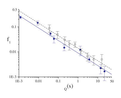
Figure 1: Log-log plot of the frequency ${\bar{f}}_{1}$ of trapping single fluxons versus the quenching time $\tau_{Q}$ for an AJTJ of circumference $0.5mm$ (closed circles) and for an AJTJ with circumference $1.5mm$. The best fits through the data (solid and dashed lines) show that scaling with $\sigma=0.5$ is totally robust. Both samples had equal critical current density $J_{c}$.

What concerns us in this paper is how fluxons form in the presence of an externally applied magnetic field $B$ that explicitly breaks the symmetry of the theory, whereby $f_{1}\neq f_{-1}$. This is a crucial ingredient in the analysis of unbiased fluxon production in JTJs because, despite our best efforts, we cannot preclude the possibility of stray magnetic fields in the experimental equipment (e.g. a magnetised screw or an incomplete shielding of the earth’s magnetic field). In fact, in presenting the data in Fig.1 we have taken the effects of static stray fields empirically into account, by applying an external field until such stray fields are neutralised. It is only then that we obtain (2). In all cases the external magnetic field $B$ was applied perpendicular to the junction plane. This choice of field orientation is mainly due to the fact that a transverse field (due to demagnetization effects) is more effective, by almost two orders of magnitude, than an in-plane field in modulating the junction critical current $I_{c}$ Monaco5 and trapping frequency. Furthermore, under particular conditions Monaco6 a transverse magnetic field allows to discriminate between fluxons and antifluxons.

As a result, we have built up a substantial collection of data showing the dependence of ${\bar{f}}_{1}$ on both $\tau$ and $B$, that we shall discuss in the remaining sections. In particular, we shall concentrate on two representative datasets that refer to high quality $Nb/Al_{ox}/Nb-Nb$ AJTJs quenched at the same quench rate ($\tau_{Q}=5s$), but having different circumferences, i.e., $C=0.5mm$ and $C=2.0mm$, shown in Fig.2 and Fig.3, respectively. Details of the samples’ electrical and geometrical parameters and of the experimental setup can be found in Monaco4 .

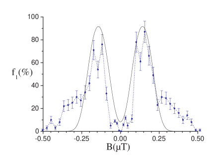
Figure 2: Dependence of the single fluxon trapping frequency $\bar{f_{1}}$ for quench time $\tau_{Q}=5s$ for an AJTJ of circumference $C=0.5mm$ in the presence of a magnetic field $B$ perpendicular to the barrier plane. The solid line corresponds to the case $N=1$ in ${\bar{f}}_{1}(N,{\bar{n}})$ of Fig.5, as derived from Eq.(22).

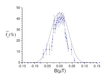
Figure 3: Dependence of $\bar{f_{1}}$ for quench time $\tau_{Q}=5s$ for an AJTJ of circumference $C=2.0mm$ in the presence of a magnetic field $B$ perpendicular to the barrier plane. The solid line corresponds to the case $N=16$ in ${\bar{f}}_{1}(N,{\bar{n}})$ of Fig.5, as derived from Eq.(22).

We observe that the increase in circumference has a dramatic effect on the single trapping frequency ${\bar{f}}_{1}$. For the $0.5mm$ long AJTJ we find a central minimum with two side-peaks. Such a double-peaked dataset has been used for any single data point in Fig.1, with ${\bar{f}}_{1}$ being read off from the central minimum, typically displaced slightly from $B=0$ because of the aforementioned stray fields in the equipment (typically several tens of $nT$).

On the other hand, for the $2.0mm$ long sample (not represented in Fig.1) we only have a central peak. Superficially this is strange, since it shows that the probability of seeing a single fluxon decreases as the external field increases, but we shall understand this as a consequence of an increased ability to create more than one fluxon. We note that the values of the magnetic field required to change ${\bar{f}}_{1}$ significantly are very small when compared to the field values needed to modulate the Josephson current $I_{c}$ of the samples, whose first minimum occurs at field values of several $\mu T$. Further, the larger the ring size the larger is the effect of a given magnetic field.

In the remainder of this paper we shall show how the results of Figs. 2 and 3 can be understood, and qualitatively predicted, in a framework that implies the scaling behavior of Fig.1. As such, these results are mutually supportive but require an alternative formulation of the KZ scenario, which we now provide.

II Causality vs. instability

At first sight the results for fluxon production in an external field have little or nothing to do with the Kibble-Zurek scenario. However, the original scenario of bounding domains by causal horizons is just one way of saying that, qualitatively, systems change as fast as is possible. From a different viewpoint we know that continuous transitions (like the one here) proceed by the exponential growth of the amplitudes of unstable long-wavelength modes of the system. This growth is strongly suppressed by self-interaction once the system is close to the ground states of its symmetry-broken phase.

Exponential growth is as fast as it gets, corresponding to linearising the equations of motion. Thus, provided there is enough time for such rapid growth before back-reaction (self-interaction) stops it, we can understand how systems can change as fast as is possible without invoking causal horizons directly. There is a corollary to this. The linear behaviour of the order parameter fields, while the transition is taking place, follows from their behaving as Gaussian random variables. In fact, for an idealised situation in which amplitude growth is stopped by implementing a rapid back-reaction that chokes off growth instantaneously, it can be shown karra ; ray ; bowick that the assumption of Gaussianity leads to scaling behaviour like that of (1), with the same values of $\sigma$ as would be obtained from causal bounds. What may seem surprising is that, even when back-reaction is included more realistically, numerical simulations lag ; moro ; ray2 show that the behaviour is still essentially the same. The $\sigma$ exponents of causal reasoning are recovered. There are, however, two major differences between fastest amplitude growth and causal bounds. The growth starts after the transition has begun, whereas causal bounds can be imposed both before or after the transition has begun, usually to the same effect zurek1 ; zurek2 . Numerical simulations show moro ; ray2 , without a doubt, that it is the behaviour of the system after the transition has begun that determines the domain structure. This is necessary in our context since, with no Josephson effect for $T>T_{c}$, we could not have invoked causality before the transition. Further, the assumption of Gaussianity gives us more than causality, in that it reintroduces the role of the Ginsburg temperature, at which thermal fluctuations become important,where appropriate. This provides one natural explanation for the failure to observe vortices in quenches of ${}^{4}He$ ray while, by a similar argument, permitting spontaneous vortex production in ${}^{3}He$ grenoble ; helsinki and superconductors technion2 .

However, since equations of motion are, by construction, causal, these viewpoints are largely complementary once these caveats are taken into account. When appropriate we will invoke both mechanisms in our subsequent discussion.

The simulations cited above are largely for systems with global symmetry breaking, simpler than superconductors. In fact, although local breaking gives a very different domain structure, the idea of the transition being driven by instabilities survives. Again, the exponents are those of causal arguments calzetta except that there is a additional mechanismrajantie for the spontaneous production of flux in which magnetic field just freezes in by itself, with behaviour very different to that of (1). For annular JTJs this further mechanism does not arise because of the thinness of the oxide layer through which fluxons protrude and the scaling behaviour of (1) and (2) is a clean prediction.

III Beyond The Linear Regime ($B=0$)

Suppose that there is no external symmetry-breaking field. As long as $f_{1}$ is significantly smaller than unity we expect the linear log-plot in $\tau_{Q}$, as seen in Fig.1. However, with $f_{1}$ bounded by unity the linear behaviour will soon break down for increasingly fast quenches. Once ${\bar{\xi}}=O(C)$ the trapping probability $f_{m}$ of finding net fluxon number $m$ (fluxons minus antifluxons) increases for $m>1$, forcing $f_{1}$ to decrease. For the remainder of this section we shall extend (2) to predictions for $f_{1}$ and higher $f_{m}$ across the whole range of $C/{\bar{\xi}}$.

Since the KZ scenario is appropriate for $B=0$, this is an ideal testing ground for our two approaches. We shall elaborate on these in turn and see that, for many purposes, they give almost indistinguishable results.

III.1 Independent domains and Gaussian probabilities

In the spirit of the KZ scenario a simple, but informative first guess as to how $f_{1}$ and other $f_{m}$ behave across the whole range of $C/{\bar{\xi}}$ is to divide the annulus into $N\geq 2$ independent (causal) domains in each of which the Josephson phase $\phi$ is a constant. We assume that there is no correlation between the values of $\phi$ in adjacent domains but, in calculating the total phase change $\Delta\phi$ around the annulus, the geodesic rule is adopted rudaz . This means that, when jumping from one domain to the other, the shortest path in phase will be taken. The result of a quench is then modelled as having the system divided up into N domains, each with a randomly chosen phase. There is nothing in this ansatz peculiar to JTJs, and it is equally applicable to superconductors. As such it is an idealisation of a superconducting loop, made out of Josephson junctions in series, that has been the object of spontaneous flux generation carmi .

Let $G_{M}(\Delta\phi)$ be the probability that the change in phase $\phi$ is $\Delta\phi$ after $M$ domain boundaries. If the system is made of only two domains, then the lack of phase correlation requires:

$$G_{1}(\Delta\phi) = \frac{1}{2\pi}\,\,\,\,\,\,for\,\,\,-\pi<\Delta\phi<\pi,$$

$$= 0\,\,for\,\,\,|\Delta\phi|>\pi.$$

In fact, the approach of using the KZ picture to set up discrete domains in which the order parameter field can take random values is one that has been used repeatedly for counting defects, at least since its introduction by Vachaspati and Vilenkin tanmay for counting cosmic strings (vortices) in the early universe. This adopts an earlier use of causal horizons by Kibble kibble2 , from which kibble1 evolved.

On increasing $N$, $G_{N}(\Delta\phi)$ is determined by $N-1$ self-convolutions of $G_{1}$:

$$G_{N}=\underbrace{G_{1}*...*G_{1}}_{N-1\,\,\,times}.$$

Applying the geodesic rule for the final step in phase (from domain $N$ back to domain $1$, the probability of ending with a phase shift of $2\pi m$ (i.e. net fluxon number $m$) is:

$$f_{m}(N)=\int_{-\pi+2m\pi}^{\pi+2m\pi}d\Phi\,G_{N}(\Phi)=2\pi G_{N+1}(2m\pi),$$ (3)

where the last equality comes from the definition of $G_{N}$.

To bring this further into correspondence with the KZ scenario, we should identify the domain size as comparable to $C/{\bar{\xi}}$ i.e. $C=aN{\bar{\xi}}$, where $a=O(1)$. The value of $a$ is not unity, since a discrete domain structure is only a crude approximation to a continuous phase at a continuous transition. Further, the result (1) assumes the causal bound is saturated, and we have already commented on systems (e.g. high-$T_{c}$ superconductors) for which the inefficiency of producing flux shows that this is not the case technion2 . To take general values of $C$ and ${\bar{\xi}}$ into account we need to generalise (3) to non-integer $N$.

$G_{N}(\Delta\phi)$ already shows rapid convergence to the Gaussian distribution that arises from the central limit theorem for $N\geq 2$. For such $N$ the obvious way to proceed is to adopt this central limit Gaussian distribution. That is, we assume that the total phase change $\Delta\phi$ around the annulus can be expressed as the sum of a random term $\Phi$ and a geodesic-rule correction $\delta\Phi$. If $\Phi$ has a normal distribution with average $\bar{\Phi}=0$ and variance $\sigma^{2}(N)$ i.e.:

$$G_{N}(\Phi)=\frac{1}{\sqrt{2\pi\sigma^{2}(N)}}\exp-\bigg{(}{\frac{\Phi^{2}}{2\sigma^{2}(N)}}\bigg{)},$$ (4)

then a simple calculation enables us to identify (4) with the central limit distribution of the self-convolutions of $G_{1}$, as described above, provided that:

$$\sigma^{2}(N)=N\pi^{2}/3.$$

The probability to trap a net number $m$ of defects will now be:

$$f_{m}(N)=\int_{-\pi+2m\pi}^{\pi+2m\pi}d\Phi\,G_{N}(\Phi).$$ (5)

Experimentally, in the absence of any external field, the most important probabilities are for finding one fluxon or one antifluxon. The frequency of no trapping $f_{0}(N)$ is:

$$f_{0}(N)=\int_{-\pi}^{\pi}G_{N}(\Phi)d\Phi=erf(\frac{\pi}{\sqrt{2\sigma^{2}(N)}}),$$ (6)

and

$$f_{\pm 1}(N) = \int_{\pi}^{3\pi}\,\frac{d\Phi}{\sqrt{2\pi\sigma^{2}(N)}}\exp-\bigg{(}{\frac{\Phi^{2}}{2\sigma^{2}(N)}}\bigg{)}.$$ (7)

Furthermore, for large $\sigma^{2}>>\frac{\pi^{2}}{2}$, say $\sigma^{2}\geq 20$, the trapping frequencies asymptotically approach zero as:

$$f_{\pm m}(N)\approx\sqrt{\frac{2\pi}{\sigma^{2}(N)}}\exp-\bigg{(}\frac{2\pi^{2}m^{2}}{\sigma^{2}(N)}\bigg{)}.$$ (8)

Finally, in the same limit, the variance of the discrete variable $n$ is:

$$\sigma_{n}^{2}(N)=\Sigma_{n=-\infty}^{\infty}n^{2}f_{n}(N)=<n^{2}>=\sigma^{2}(N)/4\pi^{2}.$$ (9)

For $N\lesssim 2$ we require a different approach and turn to the consequences of assuming Gaussian stochastic behaviour.

III.2 Gaussian correlations

If $x$ measures distance along the annulus, $\phi(x)$ is periodic (modulo $2\pi$). The fluxon number density (or winding number density) is:

$$n(x)=\frac{1}{2\pi}\partial_{x}\phi(x),$$ (10)

whereby the net fluxon number $n$ is:

$$n=\int_{0}^{C}\,dx\,n(x)=\frac{1}{2\pi}\Delta\phi,$$ (11)

where $\Delta\phi$ is the change in $\phi$.

For winding number density $n\left(x\right)$ the ensemble average of the net number of fluxons along an annulus of perimeter $C$, in the absence of an external field is ${\bar{n}}=\langle n\rangle=0.$

We do not need to adopt any particular form for $n\left(x\right)$. In the light of our earlier discussion we now assume that it is a Gaussian variable until the transition is complete, whereby all correlation functions are determined by the two-point correlation function $\left\langle n\left(x\right)n\left(y\right)\right\rangle$. That is, all we shall need for probabilities is:

$$\langle n^{2}\rangle = \int_{0}^{C}dx\,dy\left\langle n\left(x\right)n\left(y\right)\right\rangle.$$

It follows that:

$$\langle n^{2p}\rangle = \frac{(2p-1)!}{2^{p-1}(p-1)!}\langle n^{2}\rangle^{p}.$$ (12)

If $f_{m}$ is the probability of finding net winding number $m$ taking both positive and negative values), then:

$$\langle n^{2p}\rangle=\sum_{-\infty}^{\infty}m^{2p}\,f_{m}.$$ (13)

In order to invert equation (13), we construct the generating function $Z(z)$:

$$Z(z) = \sum_{p=0}^{\infty}\frac{(-z^{2})^{p}}{(2p)!}\langle n^{2p}\rangle=\exp(-z^{2}\langle n^{2}\rangle/2),$$

from (12). On the other hand, from (13):

$$Z(z) = \sum_{p=0}^{\infty}\frac{(-z^{2})^{p}}{(2p)!}\sum_{-\infty}^{\infty}m^{2p}\,f_{m}=\sum_{-\infty}^{\infty}f_{m}\,\cos mz.$$

That is, the $f_{m}$ are the Fourier coefficients of the Gaussian. In particular,

$$f_{0} = \frac{1}{2\pi}\int^{\pi}_{-\pi}dz\,\exp(-z^{2}\langle n^{2}\rangle/2)$$ (14)

and

$$f_{\pm 1} = \frac{1}{2\pi}\int^{\pi}_{-\pi}dz\,\exp(-z^{2}\langle n^{2}\rangle/2)\cos z$$

respectively.

We observe that, for large $\langle n^{2}\rangle$, where we can take the integration limits to infinity, the trapping probability falls off as:

$$f_{\pm m}\approx\frac{1}{\sqrt{2\pi\langle n^{2}\rangle}}\exp(-m^{2}/2\langle n^{2}\rangle).$$

In practice, this assumption of a Gaussian stochastic density can only be approximate, on two accounts. Less significantly, from our earlier comments, it ignores the non-linearities of the system. More importantly, it does not fully accommodate the periodicity of the annulus, to which we shall return later. Nonetheless, it will be apparent as to which results are reliable.

In contrasting Gaussian correlations and Gaussian probabilities we see that the definitions are dual to each other. In the limit of unrestricted integration (large $N$) they are identical if we identify:

$$<n^{2}>=\sigma^{2}(N)/4\pi^{2}=N/12.$$ (15)

However, for small $N$ there will be differences, as we shall see.

On inserting (15), we find that the likelihood ${\bar{f}}_{1}$ of seeing one fluxon or antifluxon is:

$${\bar{f}}_{1}(N) = \frac{1}{\pi}\int^{\pi}_{-\pi}dz\,\exp(-z^{2}N/24)\cos z,$$ (16)

whereas, assuming Gaussian probability, from (5) we find:

$${\bar{f}}_{1}(N)=erf(\frac{3\sqrt{3}}{\sqrt{2N}})-erf(\frac{\sqrt{3}}{\sqrt{2N}}).$$ (17)

We know that (16) and (17) agree for large $N$ but, as can be seen from Figures 4, the qualitative and quantitative agreement is striking over the whole range.

In Fig.4 we compare ${\bar{f}}_{1}$ as a function of $N$, as given by Eq.(16) and Eq.(17) (dashed and dotted lines) respectively; the dots are the values of ${\bar{f}}_{1}$ according to the independent sector model for some integer values of $N$ from Eq.(3). Agreement is already good at $N=2$ and very good at $N=4$.

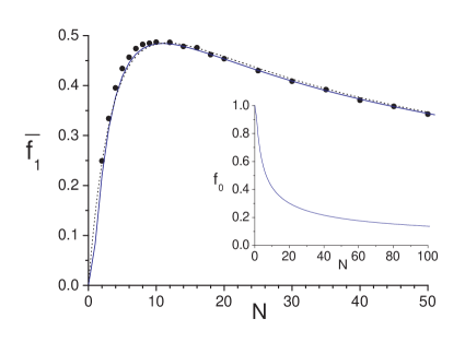
Figure 4: We display the probabilities ${\bar{f}}_{1}=f_{1}+f_{-1}$ as a function of $N$, as given by Eq.(16) and Eq.(17) (dashed and dotted lines) respectively; the dots are the values of ${\bar{f}}_{1}$ according to the independent sector model for some integer values of $N$ from Eq.(3). The maximum of ${\bar{f}}_{1}$ occurs at $N=N_{c}\approx 10.5$, for which value ${\bar{f}}_{1}\approx 49\%$. The inset shows the probability ${\bar{f}}_{0}$ as a function of $N$, as given by Eq.(6), essentially indistinguishable from that by Eq.(III.2) at this scale.

However, the plots of Fig.4 are somewhat deceptive for small $N$. This should not worry us since, although the analytic expression (17):

$${\bar{f}}_{1}(N)=O(\sqrt{N})\exp(-3/2N),$$ (18)

vanishes faster than any power, (17) breaks down there by definition. On the contrary, ${\bar{f}}_{1}(N)$ of (16) is linear in $N$ for small $N$, as we supposed in (2).

Finally, in the inset of Fig.4, we also display $f_{0}(N)$, the probability of seeing no flux, for the case of Gaussian probabilities given in (6). Although we do not show it, at the scale of the plot, it is essentially indistinguishable from the result of assuming Gaussian correlations as given in (14),

$$f_{0}(N) = \sqrt{\frac{6}{\pi N}}erf\bigg{(}\frac{\pi}{2}\sqrt{\frac{N}{6}}\bigg{)}$$

We can comfortably use either.

III.3 Consequences

In summary, the assumptions of Gaussian probabilities (as follows from the KZ picture) and Gaussian correlations are complementary, with the latter providing a (linear) interpolation of the other for $N\lesssim 2$ where the former breaks down.

The first observation is that, in both cases, the maximum probability ${\bar{f}}_{1}={\bar{f}}_{c}$ of seeing one fluxon or antifluxon is fractionally less than 50% (48.6%), occurring at $N=N_{c}\approx 10.5$. The assumption made in our JTJ papers is that ${\bar{f}}_{1}$ (which we have called $f_{1}$ in our papers) scales linearly with $N\propto C/\xi$, which we see is valid at best only until ${\bar{f}}_{1}\approx 0.3$. We have already just about achieved this in the existing experiments but have not yet been able to quench fast enough to provide a direct test of the model predictions of Fig.4. There is, however, a problem that stops us embracing the Gaussian correlation approach wholeheartedly, as we have presented it here. As we have noted, the assumption of Gaussian winding number density can only be approximate, since it does not take periodicity (mod $2\pi$) into account. We have seen that this does not matter in the calculation of $f_{0}$ and ${\bar{f}}_{1}$.

However, for small annuli there is a problem with (16) in that Fourier components $f_{\pm 2}(N)$ are slightly negative ($|f_{\pm 2}|<0.01$) for very small $N$ (with a similar problem for the very much smaller ${\bar{f}}_{4}$). On the other hand, by construction the ${\bar{f}}_{m}(N)$ of (17) are automatically positive as they must be.

In a qualitative sense it is of little consequence since, throughout the linear regime, the probability ${\bar{f}}_{>}=1-f_{0}-{\bar{f}}_{1}$, of seeing more than one fluxon is very small but, as a matter of principle, we should impose periodicity to render the probabilities positive. We do not have a reliable model in which we can do this but we can get some idea by supposing that the phase $\phi$ moved in a double-well potential rather than the periodic $\cos\phi$ potential of the sine-Gordon fluxon. In that case, assuming Gaussian correlations, the density of defects is proportional halperin to $(f^{\prime\prime}(0)/f(0))^{1/2}$, where $f(x)=\langle\phi(x)\phi(0)\rangle$. It is now straightforward to impose periodicity, whereupon we find behaviour similar to that of (18) for very small $N$, in that it vanishes faster than any power Bob . If that were to be equally applicable here it is difficult to determine when such behaviour might occur, since there is no sign of such a collapse in Fig.1, but if this analogy is correct, it will repair the minor problem of small negative probabilities while leaving the similarity between the two approaches at a quantitative level. In particular, as long as we are not looking at the small-N behaviour in too much detail, as we shall not hereafter, it becomes sensible to use the simpler Gaussian probabilities over the whole range.

IV Fluxon Production in an external field $B\neq 0$

Let us now apply a perpendicular uniform magnetic field $B$ to the AJTJ. This breaks the $\phi\rightarrow-\phi$ symmetry that is equally, the reflection symmetry of the system in the plane of the barrier. Once superconducting, the AJTJ expels the magnetic field, but we assume that a small fraction $\epsilon$ of the applied field ’leaks’ in the radial direction through the barrier, forming fluxons. The effect of this field is to produce an non-zero average winding number $\langle n\rangle={\bar{n}}(B)$.

The result is a shift in phase gradient along the annulus (coordinate $x$) of the form:

$$\partial_{x}\phi\rightarrow\partial_{x}\phi+\frac{2e}{\hbar c}A_{x},$$ (19)

where $A_{x}=A_{x}^{+}-A_{x}^{-}$ is the jump in the vector potential across the oxide layer.

If $C=2\pi R$ is the circumference of the ring, radius R, then the change in $\phi$ due to $B$ is:

$$\Delta\phi=\epsilon\frac{2e}{\hbar c}\oint{\bf dl}.{\bf A}=\frac{\epsilon}{2\pi}\frac{e}{\hbar c}C^{2}B.$$ (20)

The change in fluxon number is:

$${\bar{n}}(B)=\frac{1}{2\pi}\Delta\phi=\frac{\epsilon}{4\pi^{2}\hbar c}eC^{2}B.$$ (21)

(For future purposes, let us call $B_{1}$ the field value for which $\Delta\phi={2\pi}$, that is ${\bar{n}}(B_{1})=1$.)When ${\bar{n}}$ is small, $\epsilon$ adjusts in any individual experiment so as to make ${\bar{n}}$ integer. As a first approximation we take the fraction $\epsilon$ to be independent of $B$.

In the presence of external fields we are not primarily interested in the small $N$ linear regime and it is sufficient to work with Gaussian probabilities. The natural extension of $G(\Phi)$ of (4) for an AJTJ in a perpendicular magnetic field $B$ is that the phase distribution will still be normal with variance $\sigma^{2}(N,{\bar{n}}(B))\propto N$, where we retain the definition of $N\propto C/{\bar{\xi}}$ of the previous section, but with non-zero average $\bar{\Phi}(B)=2\pi{\bar{n}}(B)$:

$$G_{N,\bar{n}}(\Phi)=\frac{1}{\sqrt{2\pi\sigma^{2}(N,{\bar{n}})}}\exp-\frac{[(\Phi-\bar{\Phi}(B)]^{2}}{2\sigma^{2}(N,{\bar{n}})}.$$

The trapping probabilities in the presence of an external magnetic field will then be:

$$f_{m}(N,\bar{n})=\int_{-\pi+2m\pi}^{\pi+2m\pi}d\Phi\,G_{N,\bar{n}}(\Phi);.$$ (22)

To a first approximation we assume that $\sigma^{2}(N,\bar{n})$ is independent of $\bar{n}(B)$, as would follow from assuming Gaussian correlations, i.e. for integer $\bar{n}$, $f_{{\bar{n}}-m}(N,{\bar{n}})=f_{{\bar{n}}+m}({N,\bar{n}})=f_{\pm m}(N,0)$. This allows us to repeat the identification $\sigma^{2}(N)/4\pi^{2}=N/12$.

As before, we are primarily interested in the probability of seeing a single fluxon or antifluxon, but now for fixed $\tau_{Q}$ (or $N$), as a function of $B$ (or ${\bar{n}}$). Now, as far as $\bar{n}\neq 0$, then the symmetry is broken and $f_{+1}(N,{\bar{n}})\neq f_{-1}(N,{\bar{n}})$. More precisely, in Fig. 5 we show ${\bar{f}}_{1}(N,{\bar{n}})$ as a function of ${\bar{n}}$ for fixed $N$ for several $N$, as derived from Gaussian distributions Eq.(22).

Figure 5: The values of ${\bar{f}}_{1}(N,\bar{n})$ as a function of $\bar{n}$ for fixed $N$ for several values of $N$; $N=1,2,4,6,8,10,16$, according to Eq. (22).

The main characteristics of Fig.5 are that:

1. for $N<N_{c}\approx 10.5$ there is a double peak, corresponding to the ensemble average production of a single fluxon by the applied external magnetic field. This is understood as follows. Essentially, when, for $B=B_{1}$ we have ${\bar{n}}=1$, the zero-field no-trapping frequency $f_{0}(N,0)$ becomes the single fluxon trapping $f_{+1}(N,1)=f_{0}(N,0)$, giving the righthand peak for positive ${\bar{n}}\approx 1$; reversing the field, $f_{-1}(N,-1)=f_{0}(N,0)$ and we get the peak for negative ${\bar{n}}\approx-1$.The minimum value of ${\bar{f}}_{1}$ between the peaks is ${\bar{f}}_{1}(N)$, as given by the KZ scenario.

2. as $N$ increases to $N_{c}$ the height ${\bar{f}}_{1}(N,0)$drops. The variance also increases, the $\Phi$ distribution gets broader and the two peaks in $\bar{n}$ of ${\bar{f}}_{1}(N,{\bar{n}})$ merge at $N=N_{c}$ at the value ${\bar{f}}_{c}\approx 0.5$;

3. as $N$ increases beyond $N_{c}$, there is only a single peak centered on $\bar{n}=0$. We now see that the reason why the probability of seeing a fluxon decreases as $|B|$ increases is a consequence of an increased ability to create more than one fluxon.

The curves in Fig.5 for $N=1$ and $N=16$ bear a strong resemblance to the experimental data shown in Fig.2 and Fig.3, respectively. They comply with the most simple qualitative test of our analysis, that the double peaks in Fig.1 occur at a higher frequency than ${\bar{f}}_{c}\approx 50\%$, and the single peak in Fig.2 at a lower frequency than $50\%$, as predicted. Further, we also found that the defect winding number flips when we move from the left to the right peak, as foreseen by both models. This discrimination between a trapped fluxon or antifluxon can be achieved by measuring the transverse magnetic field dependence of the junction critical current $I_{c}(B)$ (the details of this new effect and its theoretical interpretation will be reported elsewhere Monaco6 ).

More specifically, we note that the $2.0mm$ long sample, being $4$ times longer than the $0.5mm$ long sample, according to (21), should be 16 times more sensitive to the externally applied magnetic field $B$, if $\epsilon(B)$ is independent of $B$ and identical for both samples. There is, indeed, a strong difference in sensitivity, but only by a factor of $7-8$, showing that these assumptions are approximate. What is more difficult to understand quantitatively is the 16-fold increase in $N$ for a four-fold increase in perimeter. This requires the efficiency factor $a$ relating $N$ to $C$ to vary by a factor of $4$ between the samples or, more fundamentally, that $N$ is not linear in $C$. Of itself, the latter does not change the scaling behaviour of (2), but the scaling exponent $\sigma$. In Monaco3 ; Monaco4 we showed that the observed value for $\sigma$ was not that for idealised JTJs KMR . We explained this as a consequence of fabrication methods, but this reopens the issue.

To go further, and match the data profiles better, we need specific properties of JTJs, beyond the generics of the KZ picture (or Gaussian correlations). In particular, the assumption of $\sigma^{2}(N,{\bar{n}}(B))$ being independent of ${\bar{n}}(B)$ is oversimple. More realistically Martucciello , $\sigma^{2}(N,{\bar{n}}(B))=\sigma^{2}(N,0)(1+k^{2}B^{2})$, where $k^{2}\propto(\lambda_{J}/C)^{2}$, i.e. it is inversely proportional to the ring area and to the Josephson current density $J_{c}$, since $\lambda_{J}^{2}\propto 1/J_{c}$. Both are consistent with the experimental data, such as the flattening of ${\bar{f}}_{1}$ for small $B$ field values and the fact that the peak amplitudes $f_{\pm n}(\pm B_{n})$ strongly decrease with $n$, as we shall see elsewhere.

V Conclusions

We have developed two complimentary theoretical approaches to understand the experimentally observed spontaneous production of fluxons on quenching annular JTJs in the presence of an externally applied transverse symmetry breaking magnetic field $B$. They either assume Gaussian probabilities (as motivated by KZ causal horizons) or Gaussian correlation functions (as motivated by models for transitions based on the rapid growth of instabilities). Both of these approaches, which are, approximately, identical, lead to the same scaling behaviour of (1), from which (2) follows in the appropriate regime.

The theory is able to nicely reproduce the double peak behavior of the likelihood $f_{1}$ to produce a single defect(fluxon) shown in Fig.2 for a sample having a circumference equal to $0.5mm$ and the single peak in Fig.3 for a sample of circumference $2.0mm$. When we began experiments on fluxon production in an external symmetry-breaking field, we anticipated the behaviour shown in Fig.2, and not that of Fig.3, which was initially incomprehensible. We now understand it, as a consequence of the ease of producing more than one fluxon in larger annuli. Specifically, our models do provide a good first approximation at a better than qualitative level and the experimental success of the Gaussian picture in describing the production of fluxons is of a piece with the scaling behaviour so robustly demonstrated in Fig.1.

References

- (1) T.W.B. Kibble, in Common Trends in Particle and Condensed Matter Physics, Physics Reports 67, 183 (1980).
- (2) W.H. Zurek, Nature 317, 505 (1985), Acta Physica Polonica B24, 1301 (1993).
- (3) W.H. Zurek, Physics Reports 276, Number 4, Nov. 1996.
- (4) R. Carmi, E. Polturak, and G. Koren, Phys. Rev. Lett. 84, 4966 (2000).
- (5) A. Maniv, E. Polturak, G. Koren, Phys. Rev. Lett. 91, 197001 (2003).
- (6) C. Bauerle et al., Nature 382
- (7) V.M.H. Ruutu et al., Nature 382, 334 (1996).
- (8) R. Monaco, J. Mygind, and R. J. Rivers, Phys. Rev. Lett. 89, 080603 (2002).
- (9) R. Monaco, J.Mygind, and R. J. Rivers, Phys. Rev. B67, 104506 (2003).
- (10) R. Monaco, J. Mygind, M. Aaroe, R.J. Rivers and V.P. Koshelets , Phys. Rev. Lett. 96, 180604 (2006).
- (11) R. Monaco, M. Aaroe, J. Mygind, R.J. Rivers, and V.P. Koshelets, Phys. Rev. B 74, 144513 (2006)
- (12) A. Barone and G. Paternò Physics and Applications of the Josephson Effect (Wiley, New York, 1982).
- (13) E. Kavoussanaki, R. Monaco and R.J. Rivers, Phys. Rev. Lett. 85, 3452 (2000). R. Monaco, R.J. Rivers and E. Kavoussanaki, Journal of Low Temperature Physics 124, 85 (2001).
- (14) Rowell et al., Can. J. Phys., 54, 223 (1976).
- (15) A.A. Golubov et al., Phys. Rev. B, 51, 1073 (1995).
- (16) R. Monaco, M. Aaroe, J. Mygind, V.P. Koshelets, arXiv: cond-mat/0706070, J. Appl. Phys., 102, 093911 (2007).
- (17) R. Monaco, J. Mygind, M. Aaroe, V.P. Koshelets, in preparation.
- (18) G. Karra, R.J. Rivers, Phys. Lett. B 414, 28-33 (1997)
- (19) G. Karra and R.J. Rivers, Phys. Rev. Lett. 81, 3707 (1998).
- (20) M. Bowick and A. Momen, Phys. Rev.D58, 085014 (1998)
- (21) P. Laguna and W.H. Zurek, Phys. Rev. D58, 085021 (1998); P. Laguna and W.H. Zurek, Phys. Rev. Lett. 78, 2519 (1997).
- (22) E. Moro and G. Lythe, Phys.Rev. E59 R1303 (1999).
- (23) N. D. Antunes, P. Gandra and R.J. Rivers, Physical Review D73, 125003 (2006)
-
(24)
A. Yates and W.H. Zurek Phys.Rev.Lett. 80 (1998) 5477-5480
Ibaceta, E. Calzetta, Phys. Rev. E60, 2999 (1999) - (25) M. Hindmarsh and A.Rajantie, Phys. Rev. Lett.,85, 4660 (2000); A. Rajantie, Journal of Low Temperature Physics,124, 5 (2001).
- (26) S. Rudaz and A. M. Srivastava, Mod. Phys. Lett. A8, 1443 (1993)
- (27) T. Vachaspati and A. Vilenkin, Phys. Rev.D30, 2036 (1984)
- (28) T.W.B. Kibble, J. Phys.A9, 1387 (1976)
- (29) B.I. Halperin, published in Physics of Defects, proceedings of Les Houches, Session XXXV 1980 NATO ASI, editors Balian, Kléman and Poirier (North-Holland Press, 1981) p.816.
- (30) A. Swarup, PhD thesis, U. of London, unpublished (2007); P. Gandra, R.J. Rivers and A. Swarup, in preparation.
- (31) N. Martucciello and R. Monaco, Phys. Rev. B53, 3471 (1996).